Modeling long term electricity forward prices

Modeling long-term electricity forward

prices

Povh, Martin and Fleten, Stein-Erik

Norwegian University of Science and Technology, University of

Ljubljana

January 2009

Online at

https://mpra.ub.uni-muenchen.de/13162/

Abstract— In contrast to forwards and futures on storable commodities, prices of long-term electricity forwards exhibit a dynamics different to that of short-term and mid-term prices. We model long-term electricity forward prices through demand and supply for electricity, adjusted with a risk premium. Long-term prices of electricity, oil, coal, natural gas, emission allowance, imported electricity and aluminum are modeled with vector autoregressive model. To estimate the model we use weekly prices of far-maturity forwards relevant for Nordic electricity market. Electricity prices experienced few substantial shocks during the period we analyzed, we, however, found no evidence of a structural break. Cointegration analysis indicates two stationary cointegrating vectors. Nord Pool price is found significant in the short- and the long-run model, while the gas price is insignificant in both. Other variables are significant only in the long-run model. The model shows some influence of the risk premium, however not on the long-term electricity forwards from Nord Pool.

Index Terms_{— Electricity prices, long-term forward prices,}

VAR modeling, cointegration.

I. INTRODUCTION

OMMODITY forward markets are normally focused on contracts with time to maturity up to 1.5 years. Since the correlation between the short-term and long-term prices is high in many markets, long-term risks can be hedged with roll-over hedging using short-term and mid-term forwards and futures. Unlike most commodities, electricity cannot be stored to any great extent. In an empirical analysis of forwards from Nord Pool, Koekebakker and Ollmar [1] show that the correlation between short-term and long-term electricity futures is low and conclude that short-term contracts are not appropriate for hedging long-term exposures in electricity markets such as long-term procurement costs and production revenues. While far-maturity exposures can normally be hedged with short-term positions, electricity companies can only properly hedge them with long-term trading. Although the liquidity of long-term electricity forwards is still often low, their maturities lie up to 6 years in the future.

Long-term electricity forward prices also serve as important information carriers in that they provide valuation signals for strategic decisions like investments, mergers & acquisitions and financing of new long-term generation assets. In recent years these decisions are also influenced by the environmental pressure on the technology shift from

M. Povh is with the University of Ljubljana, Faculty of Electrical Engineering, Ljubljana SI-1000, Slovenia (email: [email protected])

S.-E. Fleten is with the Norwegian University of Science and Technology Department of Industrial Economics and Technology Management, Trondheim NO-7491, Norway (email: [email protected])

traditional coal and nuclear to natural gas and renewable sources. Investment and disinvestment decisions are triggered by changes in the relative economics of technologies, driven by changes in underlying commodity prices. The real options theory comprehensively described in [2] is appropriate for analyzing such decisions. The real option theory suggests using forward prices instead of projected future spot prices. The use of forward prices bypasses the problem of risk adjustment of the discount interest rates, allowing the assets to be valued over time with a risk neutral pricing.

Since forward contracts are not traded far enough to be used in real asset valuation the forward prices beyond the traded horizon need to be forecasted. Extrapolation of quoted forward prices might not give the best estimate; since it ignores the available information about the long-term supply and demand. Forward contracts towards the end of the term structure are often illiquid, reducing the trust in extrapolation. More sophisticated models that focus on modeling long-term supply and demand and risk adjustment are therefore necessary to produce a better estimate of forward prices beyond the term structure. Since such models involve the understanding of what influence the prices of traded far-maturity forwards, they might also prove useful in speculative trading.

Long-term electricity prices are traditionally modeled with long-term production-cost models [3], [4]. In a restructured market, however, electricity prices do not necessarily equal production costs. Different extensions of production cost models were proposed to better reflect the real prices observed in the deregulated market. A hybrid approach, in which bottom-up models based on production cost variables are calibrated on market data, has gained increasing attention in recent years [5], [6]. Nonetheless, the literature on long-term electricity forwards is still scant, due to the lack of trusted long-term market data. Long-term forward prices are more often modeled as an extension of short-term forward-price modeling. Schwartz [7] uses models estimated on short-term oil futures and tests their performance on the available long-term oil futures. The correlation between long-long-term electricity forward prices and short- or mid-term electricity forward prices, as shown in Koekebakker and Ollmar [1], is, however, low in many markets. This indicates that short-term models are unable to explain the dynamics of long-term electricity forward prices. An example of long-term electricity forward price modeling is provided in [8], which reports on a forward-price and volatility-forecasting model that combines risk adjustment and external long-term forecasting models.

In this paper we focus on modeling the dynamic structure of long-term electricity forwards. To model these prices we try to identify the long-term information that influences the expected long-term electricity supply, demand and risk premium. We analyze the weekly prices of Nord Pool’s

long-Modeling long-term electricity forward prices

C

long-term forward prices of fuels, emission allowances and imported electricity. Due to possible endogeneity we use vector autoregressive model, which do not require any ad-hoc assumptions on exogeneity.

This paper is organized as follows. Section 2 identifies the long-term electricity forward price process. The use of the data and univariate model representation is presented in Section 3. Section IV starts with descriptive analysis of variables and multivariate representation. This is followed by cointegration analysis and estimation of vector error correction model. Section 5 draws the conclusions.

II. LONG-TERM FORWARD PRICE FORMATION

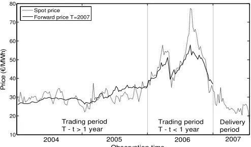
We define long-term electricity forward prices as prices of electricity forwards with a delivery period of one year and a time to maturity of more than one year (T - t ≥ 1 year).

Fig. 1 presents an example of the price dynamics for a forward contract from the Nordic electricity exchange Nord Pool with delivery in 2007. These contracts, though named forwards, correspond to the definition of swaps, having a stream of cash flows that depends on the difference between the realized spot price and the fixed contract price. We will continue to denote them forwards. Fig. 1 demonstrates that the forward-price dynamics is different from the spot-price dynamics when T >> t. As the delivery period closes (T ≈ t) the forward-price dynamics becomes more similar to the spot-price dynamics. Long-term forward spot-prices and short-term forward prices (spot prices) are, therefore, governed by somewhat different laws, which indicate the need to model them separately.

A. Setup

The non-storability of electricity has important implications on electricity trading and the valuation of forward contracts. While the cost-of-carry arbitrage is usually applied in valuation of commodity forwards, it cannot be used in case of electricity forwards, since electricity cannot be bought today at the spot price St and stored for subsequent sale at the forward price Ft,T. As an alternative to the cost-of-carry arbitrage one can use an equilibrium approach [9]

where the forward price Ft,T is the (rational) expectation about the spot price at delivery time, Et[ST] (or simply St,T) discounted with the risk-free interest rate r and the risk premium λ. Due to the uncertainty of the expected spot price, St,T, market participants require a compensation for bearing the spot-price risk, i.e., they determine their own risk premium. When individual risk preferences are matched (e.g., on the exchange) the aggregated risk premium is obtained; this is also referred to as the market price of risk. In (1) the forward price formation is therefore an equilibrium process. If one is able to obtain an unbiased estimate of the expected spot price St,T, the supply and demand for bearing the spot price risk determines the risk premium λ.

Transforming (1) to logs gives

, ,

lnFt T =lnSt T+(T−t) ln(1+ −r λ) (2)

Assuming constant risk risk-free interest rate r and risk premium λ and writing time to maturity (T – t) as Tm, (2) can be rewritten to

, ,

lnFt T =lnSt T+RTm (3)

where R is the risk premium parameter defined as ln(1 + r –

λ). In (3) the risk premium therefore depends only on time to maturity. In modeling fixed income markets, foreign exchange markets or commodity markets this is a very common assumption. In case of electricity an assumption that risk premium depend only on time to maturity is also often applied [10], despite some empirical findings, which indicate that the risk premium in short-term electricity forwards might be influenced by the probability of price spikes (load seasonality) and the level of prices [11], [12]. Some investigations, which also extends to far-maturity contracts, however, indicate that the magnitude and the variability of the risk premium in far-maturity electricity forwards is low [13], [14].

In (3) the forward prices are therefore mainly driven by the expected spot prices, subject to information sets available to market participants. We assume that information sets in our case include past information about Ft,T as well as the information that influence the expected spot price St,T, i.e. variables that influence the expected supply and demand. We assume all participants (i.e. producers, buyers and traders) have the same information set.

B. Modeling the long-term expected spot price

We define the long-term forwards as the contracts with delivery period of one year, having a payoff that depends on the realized spot price over the delivery year. The long-term expected spot price St,T therefore represents the expected price of 1 MW of annual base-load electricity. Expected electricity spot prices a few years into the future are influenced by the expected supply and demand at the delivery time T. The supply and demand are however not observable variables. Instead we can use fundamental variables that influence the supply and demand to estimate their influence on the expected spot price. Electricity demand can sufficiently be explained with weather, economic activity and demography, whereas the

10 20 30 40 50 60 70 80

Observation time

Pr

ic

e

(

€

/M

W

h

)

Spot price Forward price T=2007

2004 2005 2006 2007

Trading period T - t > 1 year

Trading period T - t < 1 year

Delivery period

variables influencing the supply can be grouped into five groups:

1. Fuel prices (coal, natural gas, oil),

2. Water-reservoir level in hydro-rich systems, 3. Emission allowance prices (CO2),

4. Supply capacity (market structure, available capacity) 5. Electricity prices in neighboring markets (in the case that

a significant share of electricity is imported or exported)

When estimating the expected spot price in the long-term we seek reliable information about the expected values of the fundamental variables mentioned above. In the short term (T ≈ t) the fundamental variables can be predicted with high, though not complete, accuracy. As the time to maturity increases, the variance of these variables increases and their mean values are harder to predict. Still, there is a difference between variables that are considered stationary and integrated variables. With stationary variables the unconditional variance is bounded and the unconditional mean is based on historical average and expected growth. Such are the hydro reservoir levels, supply capacity and electricity demand, which can be predicted based on historical average value and expected long-term growth. The unconditional mean for hydro reservoir level equals historical average reservoir level, since the weather cannot be predicted any better than using the historical average. The expected term demand can be estimated on the basis of expected long-term growth, which is influenced by economic and demographic drivers. The long-term expected supply capacity can be predicted on the basis of known plans about the commissioning of new power plants and the decommissioning of old power plants. Integrated variables on the other hand have no unconditional distribution since the shocks in these variables will persist and their unconditional variance is therefore unbounded. In our case these are fuel prices, emission allowance prices and prices of electricity in neighboring markets. Fortunately the market offers securities to hedge their uncertain future evolution. Among these securities, we use long-term forward prices of fuels, emission allowances and electricity in neighboring markets to explain the dynamics of long-term electricity price.

Information on the forward prices for fuels, emission allowances and imported electricity, changes on a daily basis, since these forwards are usually traded each working day. Information on the long-term expected demand and the expected supply capacity changes only when new information on the underlying factors (GDP, construction and retirement plans) becomes available; this information changes less frequently (e.g., monthly, quarterly or yearly). The problem with this data is also that it is not as reliable as market-based information. Unless it is published as a part of exchange information, market participants need to estimate the expected demand and supply capacity themselves. The expected spot price is, therefore, influenced by high-resolution market-based information (forward prices of fuels, emission allowances and neighboring-market electricity) and by low-resolution estimated information (expected demand and supply capacity).

Due to the different resolutions of both types of information an estimation of the influence of these variables

on electricity forward prices is challenging. In this paper we use only high resolution market-based information, whereas low-resolution estimated information is the additional source of uncertainty and influence the variance structure of expected long-term electricity spot prices. Our model for the expected long-term spot price of electricity is therefore

, , , , , , ,

ln ln fuel ln ea ln nm

t T i t T i j t T j k t T k

i j k

S =

∑

∑

∑

where St T, is the expected electricity spot price, , ,

fuel t T i

F is the

forward price of fuel i, _{, ,}ea t T j

F is the forward price of the

emission allowance j and , ,

nm t T k

F the forward price of electricity in a neighboring market k.

III. DATA AND DESCRIPTIVE ANALYSIS

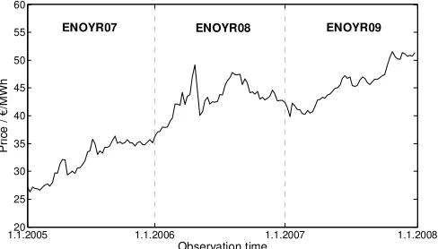
We test the proposed model on the long-term electricity forwards from the Nordic electricity exchange Nord Pool. Nord Pool is one of the oldest electricity exchanges, covering the area of four Nordic countries: Norway, Sweden, Finland and Denmark. In 2005 most of the electricity in the Nordic electricity market was supplied by hydroelectric plants (54%), with the rest coming from nuclear (22%), renewable (8%), coal (6%), natural gas (5%), imports (3%), oil (1%) and other sources (1%). In 2005 the Nord Pool financial market volume was 786 TWh, physical volume was 176 TWh, whereas the total production in the market was 404 TWh. The market went through a number of structural changes, the latest being the introduction of the European emission trading scheme (ETS) in 2005. Since this changed the overall price formation, we choose to analyze only the prices from the start of 2005 to the end of 2007. Our sample is constructed in a way to include only prices of yearly contracts with time to maturity between 1 year and 2 years as shown in Table I. For observation period 2005, ENOYR07 is used, and this contract is replaced with ENOYR08 with the start of 2006 and with ENOYR09 with the start of 2007. This way we avoid the price shift when two consecutive contracts are rolled over. Since contracts with delivery period 2 and 3 years ahead move very similar, the difference between them is very small. For other variables, defined in the following of the paper, we use forward prices with the same observation and maturity period.

The analysis of high-resolution financial data often involves the problem of non-synchronous trading. The prices in our analysis are quoted at different times, and due to the time mismatch, the integration between them is not clear. We use weekly resolution instead of daily resolution, since the relative time mismatch is much lower in the case of weekly sampling. Although the weekly sampling tends to smooth out the magnitude of price jumps, the volatility structure should

TABLEI

SAMPLE CONSTRUCTION

CONTRACT MATURITY PERIOD T OBSERVATION PERIOD t

ENOYR07 2007 2005

ENOYR08 2008 2006

sampling. We use the closing price from each Wednesday as the reference weekly price for all the variables, giving the sample size of N=156.

As shown in Fig. 2, there are no significant shifts at the time of rollover. The sample, however, shows a significant price shock in April 2006 corresponding to observations 67 to 70. Before this shock, CO2 emission allowance prices were

pushing electricity prices up significantly, however, when the report on actual emissions in EU was published in April 2006, the prices of emission allowances dropped dramatically, which had a significant effect on electricity prices. We will investigate this effect by testing whether this shock can be considered as a structural break in the relationship between the variables.

A. Fuel prices

Fuel prices can be divided into two groups, based on data availability. In the first group are the fuels that are not traded on an exchange, and so no transparent information about their prices exists. These fuels are uranium, biomass, water, wind, solar and other renewable sources. Prices of these fuels are uncertain and they influence the variance structure of electricity prices. In the second group are the fuels that are traded on an exchange, and at least some information about their long-term prices is available. These are oil derivatives, natural gas and coal. Although their use in electricity production in the Nordic market is small, they are often the marginal source of production and can have a significant influence on electricity prices. We model the fuel price _{, ,}fuel

t T i

F

with the forward prices for coal ,

coal t T

F , natural gas ,

gas t T

F and

crude oil _,oil t T

F , which also represents the price of all oil derivatives.

, , 0 1 , 2 , 3 ,

ln fuel ln oil ln coal ln gas

i t T i t T t T t T

i

F F F F

α =α α+ +α +α

∑

For the crude-oil price we use the NYMEX WTI light sweet crude oil data. Although the Brent crude oil data from the Intercontinental Exchange (ICE) might be a better choice for Nordic countries, the availability of long-term oil prices is much better at NYMEX. The long-term crude-oil price is influenced by the global long-term supply and demand. The

price indicator of the world oil price in the long term.

The steam-coal market cannot be characterized as a global market like crude oil. The majority of coal is still traded over the counter, mostly because coal is hard to standardize, due to its different energy values. Exchange forward trading with coal is still in its early stages. Instead, we use the TFS API2 index as a reference for coal prices in the Nordic area. TFS API2 is a price index for coal delivered in Amsterdam, Rotterdam and Antwerp harbor and should, therefore, also represent the coal prices in the Nordic area.

The natural gas consumed in the Nordic area comes mainly from North Sea resources. Natural gas forwards of North Sea gas is also traded on ICE. We use the ICE quarterly prices of natural gas forwards to construct the yearly forward prices for natural gas.

B. Emission allowance prices

The price of emission allowances in our model include only the price of the European CO2 emission allowance

(EUA) which were introduced by European emission trading scheme (ETS) in 2005 for carbon oxide (CO2) emissions. The

second part of (4) is therefore

, , 1 ,

ln ea ln eua

j t T j t T

j

F F

β =β

∑

where _,eua t T

F is the forward price of the EUA. We use the data on EUA prices from Nord Pool. Since Nord Pool began trading with EUAs in March 2005, we use the Spectron EUA prices which precede that date. Combining the EUA price from two different exchanges is possible, since CO2 allowance

is a global commodity that can be purchased and used anywhere in Europe. The difference in the EUA prices between Spectron and Nord Pool is negligible.

C. Neighboring-market price

The Nordic electricity market imports electricity from Russia, Germany and Poland. We have no information on import prices from Russia, so we use only the European Energy Exchange (EEX) long-term forward price as a reference price for the electricity imported from Germany and Poland. The neighboring-market price is, therefore, the EEX long-term electricity forward price.

, , 1 ,

ln nm ln eex

k t T k t T

k

F F

γ =γ

∑

We expect that the EEX price represents a rich source of information. Firstly, it influences the total market price through import and export and secondly, it could be influenced by similar information that influences the Nord Pool price.

Combining (3), (4), (5), (6) and (7) gives the following regression model describing the long-term electricity forward prices from Nord Pool.

, 0 1 , 2 , 3 , 1 , 1 , ,

ln ln ln ln

ln ln

np oil coal gas

t T t T t T t T

eua eex

t T t T m t T

F F F F

F F RT u

α α α α

β γ

= + + +

+ + + + (8)

1.1.200520 1.1.2006 1.1.2007 1.1.2008

25 30 35 40 45 50 55 60

Observation time

P

ri

ce /

€/

M

W

h

ENOYR07 ENOYR08 ENOYR09

In (8) we include an error term εt,T, which represents the uncertainty in the expected spot price and the uncertainty in explanatory variables. We assume the error term ut,T follows a normal distribution.

IV. MULTIVARIATE MODEL

Model (8) defines the univariate relationship between a dependent variable and explanatory variables on the right-hand-side. The drawback of such representation is that explanatory variables are assumed to be exogenous, which is an assumption that should be tested rather than assumed a priori. Another drawback of representation in (8) is that it fails to validly estimate all the long-term relationships between the variables, particularly when variables are non-stationary and cointegration between variables is present. In our model we cannot assume exogeneity or stationarity, since the prices of interdependent commodities are often cointegrated and non-stationary. A model that overcomes the deficiencies of single equation models is a vector autoregressive model (VAR). VAR model assumes that all variables are endogenous; hence all variables are modeled as a function of own past values and past values of other endogenous variables. We define a general Gaussian vector autoregressive model

0 ,

1 1 1

k m n

t i t i j t j j j t t

i j h

− −

= = =

= +

∑

∑

∑

Y A A Y Z w u (9)

where Yt is a vector of endogenous variables, Zt vector of exogenous variables and wj,t intervention dummies to render the residuals ut well-behaved. We use the logs of

,

np t T

F , ,

oil t T

F , ,

coal t T

F , ,

gas t T

F , ,

eua t T

F , ,

eex t T

F , as endogenous variables and we denote them as np, oil, coal, gas, eua and eex respectively. Time to maturity Tm is considered exogenous.

A. Sample analysis

Table II gives descriptive analysis of variables in (9). The variables are clearly not normally distributed; particularly the skewness in gas and kurtosis in np and gas are very high. Non-stationarity cannot be rejected in all cases except for oil and eua. Both stationarity tests are strongly reject the non-stationarity in first differences (not presented here). Variables np, coal, gas, and eex are therefore integrated of order I(1), while oil and eua may be I(0), although the results are not strongly significant.

B. VAR Setup

Based on stationarity test we will assume that none of the variables is I(2) and the system is therefore adequately modeled as I(1). The model (9) with lag length set to k = 2 is estimated and results together with diagnostics are presented in Table II. No intervention dummies wj,t are included at this point.

All endogenous variables in VAR are significant. Significance test (Fsig)on deterministic components show that constant is marginally significant, while time to maturity Tm is not. The diagnostic tests involve F-tests that there is no residual autocorrelation (Far, against 4th order autoregression), that residuals are normally distributed (χ2nd), that there is no heteroscedasticity (Fhet) and that there is no autoregressive conditional heteroscedasticity (Farch, against 4th order). Misspecification tests reveal significant problems with all of these tests, particularly when vector tests are considered. Since VAR estimates are more sensitive to skewness than kurtosis, residuals skewness is also reported.

To overcome the undesired properties of residuals in Table II we first focus on the structural specification of the model. Increasing the lag length k does not help to remove residual autocorrelation. Since residual autocorrelation also suggests an omission of important variables that influence the dynamic structure of our model, we analyze the price movement during this period and search for additional variables that might also be included in the model. Among much non-quantifiable information we find that aluminum prices also affected the prices of electricity in Scandinavia and Europe during this period. Aluminum prices rose significantly during this period and this triggered some decisions to postpone the decommissioning of some aluminum smelters, which could sell aluminum under increased long-term aluminum prices, with long-term electricity forwards as hedging instruments. The long-term aluminum prices therefore reflect changes in part of future electricity consumption and influence the demand for long-term electricity forwards. Descriptive analysis for aluminum forward price (alu) from London Metal Exchange also show a non-normal distribution, while the values of ADF and Phillips-Peron test are -1.46 and -1.28 (cv1%=-4.02) indicating integration of order I(1).

We also introduce a few dummies to the system to account for the shocks, which are known to induce erratic behavior

TABLEII

VAR(2) DIAGNOSTIC TESTS

TEST Far(4,136) χ2

nd(2) SKEW. Fhet(26,113) Farch(4,132) SE

np 1.11 19.7** -0.33 4.56** 6.81** 0.0252

oil 1.35 2.15 -0.14 1.08 0.40 0.0262

coal 3.57** 6.26* 0.26 0.90 0.55 0.0193

gas 0.82 21.3** 0.73 0.99 5.75** 0.0313

eua 0.98 11.4** 0.11 1.66* 3.79** 0.0635

eex 1.84 29.6** 0.36 2.06** 8.33** 0.0179

CONST.: Fsig(6,135) = 2.72*, Tm: Fsig(6,129) = 0.60, LLF=2207.1

VECTOR:Far(144,656)=1.37**, χ2nd(12)=59.0**, Fhet(546,1610)=1.15*

* rejects the null hypothesis at 5% significance level ** rejects the null hypothesis at 1% significance level

TABLEII

DESCRIPTIVE ANALYSIS OF VARIABLES

VARIABLE np oil coal gas eua eex

MEAN 3.68 3.87 3.94 4.12 2.94 3.90

STD. DEV. 0.18 0.16 0.09 0.24 0.29 0.17

SKEWNESS -0.71 -1.70 0.65 -0.84 -1.70 -0.92

EXC. KUR. -0.48 2.46 0.41 -0.06 3.51 -0.57

ADF TEST -2.33 -3.46* -2.03 -2.68 -3.84** -1.54

PP TEST -2.21 -3.50** -2.01 -2.56 -2.93* -1.51

set the residuals from 67 to 70, to zero, which correspond to eua price shock in April 2006. A blip dummy Db67 of a type

(…0,1,0…) with three lags is used for this purpose. Next we add one transitory dummy Dtr of a type (…0,1,0,-1,0…) to remove the effect of transitory shock in observations 27 and 29. Additionally three blip dummies Db33, Db57 and Db117 are

used to remove the largest outliers. The diagnostics of VAR that include these changes is presented in Table III.

The results in Table III show that aluminum price and dummies help to improve the properties of VAR. Most single equation and vector misspecification tests are improved. There is a still slight autocorrelation present in coal and alu, but we will not pursue this further, since we expect these two variables are weakly exogenous and they do not have to be modeled themselves. The vector tests on the other hand reject the autocorrelation and heteroscedasticity in residuals. While strict normality is still not achieved, we managed to reduce the skewness, which is more critical than kurtosis.

We test this specification for parameter constancy. In particular we are interested in the influence of eua price shock in April 2006. The shock had a significant effect on the Nord Pool forward price as seen in figure 2 and also the EEX forward price. To test whether this shock or any other shock during this period, changed the overall structure of the data

[15]. Figure 2 shows recursive break-point Chow test for each equation in the system and for the system as a whole. The 1% significance level of the break-point test is never exceeded indicating that parameters of individual equations and the system as a whole are constant throughout the sample. The eua price shock can therefore be considered as a transitory shock, which can be removed with intervention dummies, rather than a structural break.

VAR in Table III is also tested for stability by checking the roots of the companion matrix. All the roots lie inside the unit circle with the moduli of the three largest roots being 0.981, 0.981 and 0.948 respectively indicating that this representation of VAR is stable.

C. Cointegration analysis

Since unit root testing indicate that first differences are I(0), we convert the model (9) to first difference model. This model explains only the short-run dynamics of the system, while the long-run relationship between variables, which is important if variables are cointegrated, is lost. Cointegration between non-stationary variables can be captured with equilibrium error correction model:

1 0 1

1 ,

1 1

k

t t i t i

i

m n

j t j j j t t

j h

−

− −

=

−

= =

Δ = + Π + Δ +

Ψ Δ + Θ +

∑

∑

∑

Y A Y Γ Y

Z w u

(10)

which has the same innovation process ut, since no restrictions have been imposed by transformation from (9) to (10). In (10) the R.H.S. contains information about the short- and the long-run adjustment to changes in Yt. If Yt contains I(1) variables, then ΔYt-i is I(0), while ПYt-1 must also be I(0) for ut to be a white noise process. Matrix Пcan be decomposed toП = αβ’ where α represent the speed of adjustment to disequilibrium and β’ _{is the matrix of long-runcoefficients such that} β’Yt-1

represents up to n – 1 stationary cointegrating relationships, which ensure that Yt converge to their long-run steady state solution. A note however is necessary that since Yt contains two variables that are possibly I(0) in levels, they form a cointegrating relation by itself adding to the total number of cointegrating relations. A0 is unrestricted constant which

accounts for a constant in the short-run model (trend in levels) and a constant in cointegration space.

To test for cointegration between variables we employ Johansen testing procedure [16] which concentrates on testing whether the eigenvalues λi of the matrix П in (10) are significantly different from 0. We test whether П has a reduced rank r ≤ (n – 1), indicating that there are r stationary cointegrating relationships between non-stationary variables in VAR. If r = n, this would indicate that all variables are stationary, while r = 0 would indicate no stable cointegrating relationships and the VAR with first differences only would be adequate. To determine the rank r we use the trace test statistics

( )

trace

1

ˆ log 1

n

i i r

T

λ λ

= +

= −

∑

TABLEIII

VAR(2) DIAGNOSTICS TESTS

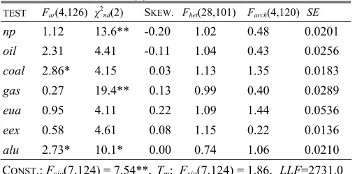
TEST Far(4,126) χ2

nd(2) SKEW. Fhet(28,101) Farch(4,120) SE

np 1.12 13.6** -0.20 1.02 0.48 0.0201

oil 2.31 4.41 -0.11 1.04 0.43 0.0256

coal 2.86* 4.15 0.03 1.13 1.35 0.0183

gas 0.27 19.4** 0.13 0.99 0.40 0.0289

eua 0.95 4.11 0.22 1.09 1.44 0.0536

eex 0.58 4.61 0.08 1.15 0.22 0.0136

alu 2.73* 10.1* 0.00 0.74 1.06 0.0210

CONST.: Fsig(7,124) = 7.54**, Tm: Fsig(7,124) = 1.86, LLF=2731.0

VECTOR: Far(196,665)=1.13, χ2nd(14)=43.4**, Fhet(784,1601)=0.86

* rejects the null hypothesis at 5% significance level ** rejects the null hypothesis at 1% significance level

0 50 100 150 0

0.5

1 np

0 50 100 150 0

0.5

1 oil

0 50 100 150 0

0.5

1 coal

0 50 100 150 0

0.5

1 gas

0 50 100 150 0

0.5

1 eua

0 50 100 150 0

0.5

1 eex

0 50 100 150 0

0.5

1 alu

Si

g

n

if

ic

an

ce

/

%

0 50 100 150 0

0.5

1 system

Breakpoint

where T is the sample size and λˆi are the estimated

eigenvalues of П. The results of the cointegration rank test, presented in Table IV, show that λ1 is strongly significant

while λ2 and λ3 are on the borderline of significance with p

values 0.019 and 0.074 respectively. It is hard to know exactly if they form a stationary cointegrating vector or not.

Since the choice of cointegration rank is crucial in modeling cointegrated systems, we look for additional indicators for determining r, as specified in [17]. First we look at the moduli of the largest characteristic roots of the model, and see how they are changing for the hypotheses in question, i.e. r = 1, 2 and 3. Table IV again show indecisive results for r = 2 and r = 3. It is hard to know exactly whether a moduli of 0.910 represent a unit root or not. Next we look at the significance of parameters of loading matrix α. The t-value of

α2,2 is -4.20 and for α5,3 is -3.28 indicating that the second

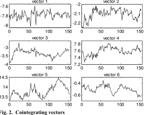
vector adds additional explanatory power to the oil equation and third cointegrating vector to the eua equation. Finally we look at the graph of the first six cointegrating vectors presented in Fig. 2.

The first two cointegrating vectors look stationary and the last three are clearly not. For the third cointegrating vector it is hard to decide, so we test the third vector with ADF test and Phillips-Perron test. Both of them reject stationarity with probability of 0.115 and 0.153 respectively. Based on these finding we choose cointegration rank r = 2. Although the third

vector might also help explain the long-term relationship in eua equation, it is not stationary.

To identify the two vectors we test the restrictions on estimated α andβ. We first rotate the cointegration space by normalizing β with respect to np and oil. This way beta is exactly identified and the significance of each variable in cointegration space can be tested by putting additional restrictions on parameters in β. These tests based on standard LR test show that in the second vector only the oil parameter is significant, indicating that the second vector is exactly oil, consistent with the unit root test results showing oil being stationary in levels. The first cointegrating vector is a linear combination of np, coal, eua, eex and alu. Gas price is insignificant in both cointegrating vectors and therefore have no long-run explanatory power. Testing all the restrictions gives the following representation of β, with the standard errors below.

( ) ( ) (0.10) ( ) (0.03) (0.17) (0.16) ( )

( ) ( ) ( ) ( ) ( ) ( )

ˆ _{1 0 0.72 0 0.13 0.93 0.96}

0 1 0 0 0 0 0

np oil coal gas eua eex alu

− − −

−

− − − − − −

⎡ ⎤

⎢ ⎥

=_⎢ − − _⎥

⎢ ⎥

⎢ ⎥

⎣ ⎦

β

In the second step we test the restrictions on loading matrix α,which is also known as the test for weak exogeneity. The test involves testing the restrictions that particular row in the estimated loading matrix α is insignificantly different from zero. The parameters of α explain how the short-run model (i.e. the first difference model) is adjusted to the disequilibrium represented by cointegrating vectors β’Yt-1. If

the entire row in α is zero this indicates that none of the cointegrating vectors enter the equation associated with this row. This equation can therefore be excluded from VECM, and this variable is called weakly exogenous. Testing these restrictions additionally to restrictions on β shows that coal and alu are weakly exogenous in our model, while other variables are endogenous.

Based on cointegration test and weak exogeneity test we form a VECM as in (10). Yt now includes endogenous variables np, oil, gas, eua and eex, while Zt includes two weakly exogenous variables coal and alu and time to maturity Tm. Estimation of (10) includes one lag of first differences of endogenous variables, the first lag of two cointegrating vectors, the first lag of weakly exogenous variables, eight dummy variables and a constant, giving 25, 10, 15, 40 and 5 parameters respectively, a total of 95 parameters to estimate. We reduce the model size with the standard F-test, which seeks the balance between the goodness of fit and the degrees of freedom. The reduced model shows that gas is also insignificant in the short-run model so we completely remove gas from the system. The 4 dimensional model now include 40 parameters and the value of F-test on reduction is F(30,526)=1.06. The reduced model includes the first lag of

Δnp, two cointegrating vectors, a constant, ΔTm and five dummies only. The diagnostic tests presented in Table V show that the main properties of residuals remained unchanged with standard errors very close to values in Table III. Since coal, alu and gas equation are removed from the system, vector autocorrelation and heteroscedasticity tests are improved. Normality test, however, show no improvement. Both

0 50 100 150 -8

-7.8 -7.6

vector 1

0 50 100 150 -2.2

-2.1

-2 vector 2

0 50 100 150 -4

-3.5 -3

vector 3

0 50 100 150 7.2

7.4 7.6 7.8

vector 4

0 50 100 150 13.5

14

14.5 vector 5

0 50 100 150 -0.6

-0.4

vector 6

Fig. 2. Cointegrating vectors

TABLEIV

COINTEGRATION RANK TEST AND CHARACTERISTIC ROOTS

H0:rank≤ λi λtrace prob r = 1 r = 2 r = 3

0 0.372 172.5** 0.000 1.000 1.000 1.000

1 0.196 101.0* 0.019 1.000 1.000 1.000

2 0.177 67.47 0.074 1.000 1.000 1.000

3 0.114 37.55 0.326 1.000 1.000 1.000

4 0.074 18.92 0.509 1.000 1.000 0.910

5 0.027 7.11 0.572 1.000 0.871 0.910

6 0.018 2.85 0.091 0.405 0.431 0.458

the choice of cointegration rank is correct. ΔTm is significant only in Δeua and Δeex equation indicating that the system show some influence of the risk premium, however the significance is strongly rejected in Δnp (p=0.70), which is in our interest.

V. CONCLUSION

We have analyzed the long-term electricity forward prices using a vector autoregressive model. The model is specified based on variables that influence the expected long-term electricity supply, demand and risk premium. We use the long-term forward prices of oil, coal, natural gas, emission allowances, imported electricity and aluminum prices to model the dynamic properties of long-term electricity forward prices. The risk premium is modeled as a function of time to maturity.

The model is estimated on weekly data from 2005 to 2007 using variables relevant for Nordic electricity market. We specify a 7 dimensional VAR with two lags and few intervention dummies to render the residuals well behaved. The influence of emission allowance price shock in April 2006 is analyzed with Chow breakpoint test. The test show no breaks in constant or trend. The variables in the model are all integrated of order I(1), except oil and emission allowance price, which are close to I(0). The system is tested for cointegration using Johansen cointegration test. The test, together with other indicators, indicate two stationary cointegrating relationships, the first being a linear combination of non-stationary variables and the second being exactly the oil price. Gas price is found insignificant in both the short-and the long-run model. The model show some influence of risk premium, however its influence on electricity forward prices from Nord Pool is not confirmed. This indicates that the risk premium dynamics in the long-term electricity forwards from Nord Pool is rather low and that the risk premium could be considered as constant. While these results hold for the Nordic electricity market, other markets may have a different maturity level and their price dynamics may respond to other variables. Nevertheless, the general approach could be used for analyzing other electricity markets.

The authors wish to thank Nord Pool ASA for the access to their FTP database and Sjur Westgaard, Jens Wimschulte, Stein Frydenberg and Nico van der Wijst for helpful comments. Fleten acknowledges support from the Research Council of Norway through project 178374/S30.

REFERENCES

[1] S. Koekebakker and F. Ollmar, “Forward curve dynamics in the Nordic electricity market,” Managerial Finance, vol. 31, no. 6, pp. 74-95, 2005. [2] A. K. Dixit and R. S. Pindyck, Investment under uncertainty, New

Jersey, Princeton:Princeton University Press, 1994.

[3] J. A. Bloom and L. Charney, “Long range generation planning with limited energy and storage plants, part I: production costing,” IEEE Trans. on Pow. App. And Sys., vol. PAS-102, no. 9, pp. 2861-2870, 1983.

[4] S. A. McCusker, B. F. Hobbs and Y. Ji, “Distributed utility planning using probabilistic production costing and generalized benders decomposition,” IEEE Trans. on Power Systems, vol. 17. no. 2, pp. 497-505, 2002.

[5] A. Eydeland and K. Wolyniec, Energy and power risk management, Chichester: John Wiley & Sons, 2003, ch. 7.

[6] P. L. Skantze, M. Ilic, A. Gubina, “Modeling locational price spreads in competitive electricity markets: applications for transmission rights valuation and replication,” IMA J. of Management Mathematics, vol. 15, pp. 291-319, 2004.

[7] E. S. Schwartz, “The Stochastic Behavior of Commodity Prices: Implications for Valuation and Hedging,” J. of Finance, vol. 52, pp. 923-973, 1997.

[8] V. Niemeyer, “Forecasting long-term electric price volatility for valuation of real power options,” in Proc. of the 33rd _{Annual Hawaii} International Conference on System Sciences, Hawaii, 2000.

[9] R. L. McDonald, Derivatives Markets (Second Edition), Boston, MA, Addison-Wesley Series in Finance, 2006, pp. 72.

[10] S. Wilkens and J. Wimschulte, “The pricing of electricity futures: Evidence from the European energy exchange. Journal of Futures Markets, vol. 27, no. 4, pp. 387-410, 2007.

[11] H. Bessembinder and M. L. Lemmon, “Equilibrium pricing and optimal hedging in electricity forward markets,” J. of Finance, vol. 57, no. 3, pp. 1347–1382, 2002.

[12] F. Longstaff and A. Wang, “Electricity forward prices: A high-frequency empirical analysis,” J of Finance, vol. 59, no. 4, pp. 1877-1900, 2004. [13] F. Ollmar, “Empirical study of the risk premium in an electricity

market,” Norwegian School of Economics and Business Administration Working Paper. 2003.

[14] P. Diko, S. Lawford and V. Limpens, "Risk Premia in Electricity Forward Prices," Studies in Nonlinear Dynamics & Econometrics, Vol. 10, no. 3, pp. 1358-1358, 2006.

[15] G. Chow, “Tests on Equality between sets of coefficients in two linear regressions”, Econometrica, vol. 28, no. 3, pp. 591-605,1960.

[16] S. Johansen, “Statistical Analysis of Cointegrating Vectors,” Journal of Economic Dynamics and Control, vol.12, no. 2/3, pp-231-254, 1988. [17] K. Juselius, The Cointegrated VAR model: Methodology and

Aplications, Oxford, Oxford University Press, 2006.

TABLEV

DIAGNOSTICS TEST OF VECM

TEST Far(4,140) χ2

nd(2) SKEW. Fhet(14,129) Farch(4,136) SE

Δnp 1.02 22.3** 0.13 0.87 0.93 0.0198

Δoil 0.45 5.97 -0.11 0.86 0.79 0.0258

Δeua 0.85 1.02 0.21 0.82 2.42 0.0527

Δeex 1.56 9.46** 0.13 1.37 0.95 0.0134

Δnp-1: Fsig(4,141) = 3.15* ΔTm: Fsig(4,141) = 4.26**,

1 1

ˆ

t−

′

βY : Fsig(4,141) = 13.7** βˆ′₂Yt−₁: Fsig(4,141) =13.6**

CONST.: Fsig(4,141) = 13.7** LLF= 1496.5

VECTOR:Far(64,491)=1.09; χ

2

nd(8)=36.3; Fhet(140,1001)=1.08 * rejects the null hypothesis at 5% significance level