Building and Using a Small Macroeconometric Model: Klein Model I as an Example

Building and Using a Small

Macroeconometric Model: Klein Model I

as an Example

Renfro, Charles G

1 January 2009

Building and Using a Small

Macroeconometric Model:

Klein Model I as an Example

A MODLER Workbook

Charles G. Renfro

Information in this document is subject to change without notice and does not represent a commitment on the part of the publisher or the manufacturer. The software and associated files this manual describes are furnished under a license agreement by explicit contract and any use other than on the basis of a written contract between the original vendor and the distributor or purchaser prima facie constitutes an infringement of the copyright. The man-ual and the software and associated files each may be used or copied only in accordance with the terms of that contractual agreement. It is against the law to copy this software or associated files or manual onto cassette tape, disk, CDROM, or any other medium for any purpose other than the distributor’s or purchaser's private use, or the personal use of the dis-tributor’s or purchaser's employees.

 _{Copyright 2001-2009 Charles G. Renfro. All Rights Reserved}

All rights reserved. No part of this publication can be reproduced, stored in a retrieval sys-tem, or transmitted, in any form or by any means, electronic, mechanical, photocopying, re-cording, or otherwise, without the prior written permission of the copyright owner. This copyright covers not only the presentation of information in this manual, but also the asso-ciated program or programs’ human interface, command syntax and the way in which the commands are ordered to form the product as a whole.

LIMITED WARRANTY

Neither the manufacturer nor the distributors of the MODLER software shall have any ability or responsibility to the purchaser or any other person or entity with respect to any li-ability, loss, or damage caused or alleged to be caused directly or indirectly by this product, including but not limited to any interruption of service, loss of business or anticipatory profits or consequential damages resulting from the use or operation of this product. This product will be exchanged within twelve months from the date of purchase if it is found to be defective in manufacture, labeling, or packaging; but except for such replacement the li-cense of this software is without warranty or liability.

The above is a limited warranty and the only warranty made by the manufacturer, pub-lisher, or distributors of the MODLER software. Any and all warranties for merchantability or fitness for a particular purpose are hereby excluded.

Trademarks Acknowledged

MODLER, MODLER BLUE, MODLER MBA, DATAVIEW and their derivatives are trademarks of C.G. Renfro & Associates. LOTUS 1-2-3 and WordPro are trademarks of Lotus Development Corporation. Quattro Pro and WordPerfect are trademarks of Corel Systems. Excel, MS-DOS, and Word are trademarks of Microsoft Corporation. All other product names in this publication are trademarks or registered trademarks of their respec-tive owners.

Servicemark

Contents

Introduction………....1

Technical Note………...7

Chapter 1 Building the Model: First Steps……….….9

Building a Model: Basic Facilities………...13

Entering New Equations: The Identities………..18

Estimating the Behavioral Equations………. .22

Chapter 2 Forming the Model……….35

Further Elaboration of the Model…...………37

Selecting the Model………..40

Compiling the Model………....40

Creating a Solution File: Background Information…..…44

Creating a Solution File: Practical Matters………...47

Solution File Bookkeeping...………54

Additional Information……….56

Documenting the Model: The DEF File….…………..…57

Chapter Appendix: Forming an Objective Function……62

Chapter 3 Solving the Model: The Basics………..65

The First Solution: An Insample Simulation………67

The First Simulation: A Comparison………74

Predicting the Future: An Ex Ante Prediction…………..82

Chapter 4 Creating Presentations with Model Results…...101

Presenting the Model Publicly……….……...101

Creating and Editing Spreadsheet Tables……….….….105

Using a Predefined Workbook/Worksheet……….118

Appendix Using Macros to Build the Model………121

The small econometric model known as Klein Model I, or sometimes the Klein Interwar Model, was created by Lawrence R. Klein in the mid to late 1940s and first published in 1950 in Cowles Commission monograph No. 11, Economic Fluctuations in the United States 1921-1941 [19]. This model has since been a favorite of econo-mists, essentially because of its tractability, particularly when parameter estimation methods are considered. There are a number of textbooks that describe it or provide parameter estimates for it, including those by Christ [6], Desai [7], Goldberger [13], Intriligator et al [17], and Theil [31]. There have also been one or two attempts to use the model to study the policies pursued during the depression years of the 1930s. A characteristic of this model is that it is one of the simplest possible examples of a rea-sonably complete, closed economic model, straightforward enough to be described in a few pages, yet containing both important accounting identities — particularly the embryonic GNP identity — and familiar behavioral equations — specifically those for Consumption and Investment.

Employing Klein Model I as an example, this workbook describes the process of building and using an econometric model in the context of the MODLER software. As this document illustrates, quite a lot can be learned from this application about the general process of estimating, forming, and even solving a structural macroeconomet-ric model, notwithstanding Model I’s simplicity. But the Klein model also carries with it some flavor of an earlier time, which in certain respects adds interest. One as-pect is the time period itself: the fact that the model refers to the now almost fabled pe-riod of the 1920s and 1930s adds interest from that circumstance alone. However, there is also interplay between the creation of the database and the model. Any mac-roeconometric model presupposes the existence of an economic database, but this model dates from the relatively early days of national income accounting. The data used with it had to be collected and organized as an integral part of the model building process, which the 1950 monograph describes in considerable detail. The extent of this discussion reflects that the creation of the Klein model, which occurred mainly during the years 1944-47, was contemporaneous with the initial organizational devel-opment of the US National Income and Product Accounts.

sta-tistical agency and other sites. However, the absence of a requirement to collect these data observation by observation does not mean that it is no longer necessary to under-stand their characteristics. Quite to the contrary: the greater separation of the database development from the tasks of model construction both implies a need for the model builder to study the work of the economic statistician, now a specialty in itself, and raises the question of the degree to which the currently more available data base pro-vides the most appropriate data for the purpose of the model [14, 27]. In 1950, Klein characterized the then existing economic statistics as having “been prepared on the ba-sis of intuitive concepts without regard to specific models of the system from which the data are derived; consequently, there is a serious lack of coordination between the econometrician and the national income statistician. The readily available economic time series are almost never in a form suitable for immediate use in econometric stud-ies” [19, p. 123]. Although it is now usual to build econometric models essentially to fit the estimates produced by statistical agencies, reflecting ostensibly greater coordi-nation between the econometrician and the statistician, these data still do not necessar-ily provide the best foundation for model building.

In any case, the process of building an econometric model, once the data are ob-tained, involves specifying and defining the equations of the model, which immedi-ately requires a classification of the variables, and thus the data. A model’s equations can of course generally be classified into two categories, at least in the case of simple models: identities and behavioral equations. Broadly speaking, the identities express the accounting relationships that define the framework of the model. For instance, Gross Domestic Product, in usage more modern than GNP, is the sum of Consump-tion, Investment, and Government Expenditures, at least in the absence of foreign trade. The current capital stock is equal to the existing capital stock at the end of last year, plus the investment in capital stock that has occurred this year, less the deprecia-tion that occurs. Notice that such a descripdeprecia-tion of these identities conveys immedi-ately both that the model involved is a closed model and that it abstracts from certain realities. All models at best approximate the object they represent, raising instantly the question how good they are as approximations.

outset, but not yet answered—about the necessary degree of approximation before it is possible to begin to describe a model as a good, or even adequate representation of the real world.

There are a number of issues that such qualitative judgments involve, including the range of variables present in a model, the degree of their aggregation or disaggrega-tion, and how the behavioral equations should be specified. This latter topic is inti-mately related to the estimation of the parameters of the model, inasmuch as behav-ioral equations by their nature exhibit numeric parameters, the values of which are unknown and must be estimated using statistical methods. The process of estimating a model’s parameters generally begins with regression, a broadly applied statistical technique, but it does not end there. The study of the methods of parameter estimation has of course become its own disciplinary specialty over the past more than 70 years, known as econometrics, and now involves making a choice from a considerable vari-ety of estimation techniques and related statistical tests [30].

Part of the explanation for this continuing concentration on parameter estimation, even until the present day, is the historical computational environment. Klein Model I effectively predates the electronic computer. Both ENIAC, the first (programmable) electronic computer and EDVAC, the first stored-program computer, were created in the 1940s, but the earliest use of any such computer by economists (the EDSAC, a sib-ling of the EDVAC) did not occur until the early 1950s [28]. Furthermore, even until the mid-1980s, well after computers became commonplace, the process of building an econometric model of any size involved considerable time and hands-on computa-tional effort, apart from conceptual design issues. Descriptions of model building pro-jects undertaken during the 1960s and well into the 1970s usually characterized this process as necessarily involving 10 to 15 economists and research assistants for time periods of as much as a year or more, in order to construct a model of 100 or 200 equations [22]. In the 1960s and 1970s, one of the reasons was the lack of easily ac-cessible data, and in addition the lack of adequate computing facilities [28]. At the birth of the microcomputer in the late 1970s, users of even mainframe computers ordi-narily had access to less than 640K of RAM (Random Access Memory). In contrast, today, “ultraportable” notebook computers commonly offer 100 times this amount; some provide more. And throughout those years, more often than not, it was neces-sary to keypunch the data from printed documents; it was only in the 1990s that eco-nomic data became widely available in machine-readable form and, in particular, eas-ily downloaded from the Internet.

these tasks, except that the fact that mainframes were then shared facilities meant that as much as 1-8 hours or more might pass for the results to be distributed by the com-puter operator to the individual user. During these years it was also generally neces-sary for a user to be a relatively experienced computer programmer, due to a general lack of readily available software. Consequently, as an ordinary experience, it was not until 1985, or even later, with the widespread diffusion of the microcomputer, that the

typical user of a computer could expect to run a regression and obtain the results in less than a minute. Your experience will be even better: if you perform the examples as you read this document, you should find that nothing you do will take more than few seconds to perform, possibly only nanoseconds. This will be true whether your computer uses a (now “ancient”) Pentium, the latest Intel Core Duo, or one of the quad core CPUs just on the verge of becoming available.

The MODLER software described in this document has played an active part in this productivity gain. It has been used interactively on networked computers since the first months of 1970. Since the early 1980s, it has been used worldwide, dating from the time it was first “ported” to the original IBM Personal Computer, or PC, as this type of microcomputer has come to be known [1]. The initial development of this software occurred in 1968 on an IBM 7040 mainframe computer [26]. The first inter-active version was developed in 1969 and, at the beginning of 1970, was mounted on a Digital Equipment Corporation PDP-10 time-sharing mainframe computer at the Brookings Institution in Washington, DC; unusually for the time, terminals hardwire-linked to this machine were installed in offices and spaces throughout the Brookings and adjacent buildings. The specific impetus to develop this version of MODLER was to provide software to estimate the Brookings Quarterly Econometric Model of the United States on that new machine. However, once installed, it began to be used gen-erally by Brookings economists and others. In 1970, MODLER thus became one of the first production examples of an interactive, multi-user computer program. It is the first interactive statistical or econometric software package, being also one of the first computer programs to offer free-format interpretive commands [29].

the form of the Wharton PC-Mark7 Quarterly Econometric Model of the United States, a 250+ equation model, becoming a component of the first microcomputer-based economic forecasting service. In early 1985, it was used to estimate and solve the Wharton Mark VII 600+ equation model, which at the time many doubted could be estimated and solved on a microcomputer. Since then, versions of the software have been used to solve models of up to approximately 3500 equations in size, although the standard version is limited to 1000 equations.

In addition to Wharton Econometric Forecasting Associates, MODLER was adopted in the 1980s by such well-known US economic consulting firms as Chase Econometric Associates, Data Resources Inc, Lawrence Meyer and Associates, and Townsend Greenspan & Company, as well as by clients of these firms and many oth-ers worldwide. By the late 1980s, MODLER was in use in such European countries as Belgium, Denmark, France, Germany, Greece, Italy, the Netherlands, Norway, Spain, Sweden, and the United Kingdom, as well as in Africa, Australia, Canada, Central and South America, Mexico, the Middle East, Japan and Singapore. Among the types of users, it is now used in brokerage firms, central banks, corporations, and universities, as well as by local, national, and international organizations and governmental agen-cies.

However, this description does not entirely convey the essential characteristic of the microcomputer computer revolution of the past 30 years, which is the degree of repli-cated use it supports. Prior to 1980, mainframe computers were lorepli-cated in many places around the world and some of these could be accessed from a dial-up telephone link from virtually anywhere, providing in principle worldwide use. However, the significance of the personal computer is that with the advent of this technology, it be-came commonplace for the first time to transfer copies of software and models from one computer to another, thus allowing the creation of a true worldwide community of users. As early as 1970, or before, it was possible to move a model from one machine to another, but not easily; often this conversion involved considerable additional pro-gramming and was a rare event. The truth is, other than Klein Model I, very few econometric models were ever mounted on more than a single computer prior to Octo-ber 1984 [18].

A further reason, perhaps, is the relatively uninteresting operational characteristics of many of these models historically, as compared to those ostensibly offered by the inoperative theoretical models that inhabit the literature. In order to help to bridge this conceptual gap, a document parallel to this one has been created that describes the characteristics and use of an interesting series of operative theoretical structuralist eco-nomic models that are described in a new book by Wynne Godley and Marc Lavoie,

Monetary Economics [10, 11]. These particular models are not econometric models and are not estimated; the values of their behavioral parameters are simply assumed. However, once an operative theoretical model of this type has been created, the process of using it is actually quite similar to using a macroeconometric model.

Monetary Economics provides the logic and details of the construction of these mod-els. Consequently, once you have worked through the present document, you might find it interesting as a next step to look at the companion workbook, Building and Us-ing Theoretically Defined Operative Economic Models: The Godley-Lavoie Models as Examples, which can be downloaded from the Learning Tools page of the

www.modler.com website. As you will see from the Preface of Monetary Economics, MODLER was from the first used by its authors to create these models.

Technical Note

This workbook is designed to be used with all recent versions of the MODLER software, beginning with version 10.7, build 1. The software is sometimes distributed together with a CD-ROM that contains a collection of MODLER compatible files. These are contained in a self-extracting file called KMODEL.EXE. Alternatively, this self-extracting file can instead be downloaded directly from the Learning Tools sec-tion of the www.modler.com Internet website.

The files included in the file KMODEL.EXE are:

KLEINBNK.BNK 03-07-03 12046 KLEIN1.MOD 03-07-03 38138

KIDENT.MAC 02-24-03 136 ESTMOD.MAC 02-24-03 202 TSKLEIN.MAC 02-24-03 330

ESTMOD.TXT 03-07-03 5891

The date of creation of each of these files is here given for reference in US date format (mm/dd/yy); the number to the right of the date is the size of the file in bytes.

The first of these files, KLEINBNK.BNK, is a MODLER compatible data bank that contains the data necessary to create and/or use Klein Model I with MODLER. These data are annual in observation frequency and span the period from 1920 to 1941. The values are replicated from Lawrence Klein’s Cowles Commission monograph No. 11,

Economic Fluctuations in the United States 1921-1941 [19], page 135. The second file, KLEIN1.MOD, is the complete model, contained in a MODLER model file, col-loquially known as a MOD file from its extent. These two files together are sufficient to create a working version of Klein Model I; in fact, if you wish to skip the estimation of the model and to consider it beginning at the model-use stage, then go directly to Chapter II of this workbook.

first of these, KIDENT.MAC, contains the identities for the model. The second, ESTMOD.MAC, contains the code necessary to estimate the behavioral equations of the model using Ordinary Least Squares as the estimation method. The third, TSKLEIN.MAC, contains the code necessary to estimate these equations using Two Stage Least Squares. Finally, the fourth file, ESTMOD.TXT, is simply a text file that briefly describes the process of creating Klein Model I using these other files; it is in-cluded for self-documentary completeness and is redundant when you use the present workbook.

Generally this workbook presumes that you already are familiar with the MODLER software, to at least a degree. If you are not, the MODLER Getting Started Guide, the main MODLER User Guide, and the online MODLER helpfile, accessible while using the program – all of which can be downloaded from the www.modler.com website – are together intended to be used as a means of becoming more generally familiar with the MODLER software prior to reading the present workbook. This workbook is not _a

substitute for these other documents; it complements them. Furthermore, you are best advised to have read at least the MODLER Getting Started Guide, inasmuch as it de-scribes not only the website-based automatic updating of the program, as improve-ments are incorporated, but also the MODLER facilities that permit the ancillary use of word-processing, spreadsheet, Internet browser, and other programs likely to be found on your machine.

Chapter 1 Building the Model: First Steps

Klein Model I consists of three identities, expressing the accounting framework of the model, and three estimated equations, generally behavioral in type. This chapter introduces the model and describes its specific structural characteristics, but after a brief introductory discussion the chapter’s predominant focus is actually upon the step-by-step process of creating a working macroeconomic model using the MODLER software; it is not so much concerned with the conceptual whys and wherefores of the model’s particular structure as it is about this process. The Klein model is described in the Cowles Commission monograph No. 11, Economic Fluctuations in the United States 1921-1941 [19], as mentioned earlier. More modern treatments and evalua-tions include that in Berndt [4, chapter 10], Intriligator, Bodkin and Hsiao [17] and Desai [7]. The model is also described in Bodkin, Klein, and Marwah [5] in the con-text of an evaluation of the historical development of macroeconometric models gen-erally.

Using MODLER’s syntax for mathematical expressions, Klein’s original statement of the estimated model [19, p. 67ff] can be presented in terms of the following 6 equa-tions:

CE = 0.80*(W1+W2) + 0.02*PI + 0.23*PI(-1) + 16.78 I = 0.23*PI + 0.55*PI(-1) - 0.15*K(-1) + 17.79

W1 = 0.42*(Y+TAX-W2) + 0.16*(Y(-1)+TAX(-1)-W2(-1)) + 0.13*(T-1931) + 1.60

Y = C + I + G - TAX PI = Y – W1 – W2 K = I + K(-1)

where the endogenous variables are:

Y = income and net output (private net national product at market prices, net of business taxes)

I = net investment W1 = private wages PI = profits

K = capital stock, at year end

and the exogenous variables are:

G = government nonwage expenditure W2 = public wages

TAX = business taxes

T = time in years (that is, 1920, 1921, …)

Considering this model first simply as a set of simultaneous equations, the endogenous variables are mathematically the “dependent” variables, particular values of which can be generated by a “solution” of the model. The exogenous variables are the “inde-pendent” variables, the values of which must be determined in advance, before any model solution can be made. As to these variables’ characteristics as economic meas-urements, except K and T, all are flows per year, measured in billions of dollars of 1934 purchasing power. K, a stock, is also measured in billions of 1934 dollars. Time, which appears only in the term T-1931, is therefore measured in deviations from 1931. Notice also that, because the equations are provided in vector notation, lagged values are expressed simply as negative offsets, -k, where k is the order of the lag, rather than by using the notation t-k.

Although the equations are written in a slightly different form than in a printed eco-nomics text, including the absence of Greek letters, subscripts, superscripts, and other such familiar embellishments, MODLER’s syntax is nevertheless sufficiently close to standard mathematical notation that you should be able to decipher it immediately. However, there are a few important interpretative differences involved, the most sig-nificant of which is the possibly less-than-obvious fact that the equals sign here is an

operator, not just a symbol expressing equivalence. This operator quality of = is why the first and second identities (equations four and five) are stated as they are, rather than as did Klein (p. 68), who, in a non-operative written context, expressed them as:

Y + TAX = C + I + G

and

Y = PI + W1 + W2.

mathematical statement is not just a declarative statement, it is generally a command to the program to perform some operation. However, in order for this type of operation to be performed by a program, it must first be able to interpret such expressions syn-tactically, applying mathematical logic. Second, it must be able to retrieve each of the original variable values from some data source and, once the computations are made, store these values as well until they can be displayed or used otherwise.

The idea that written expressions can stand for an evaluated set of numeric values is so familiar and well integrated into modern scientific thought that this particular aspect probably will not strike you as in any way new or novel, but what is actually relatively new — a result of the invention and development of the electronic computer — is the fact that these expressions can be operative, not just symbolic. The syntax in operative form takes a little getting used to: in particular, from the start you need to be aware that, implicitly or explicitly, the computer must be told how to operate with the infor-mation that you provide it, which may either require a little more from you, or else the prior establishment of a default convention. For example, when writing an equation, it is usually easiest, in the sense of being most parsimonious, to use the explicit (normal-ized) form, as above. However, as software, MODLER is sufficiently sophisticated that, in the context of a model, were you initially to write the first identity above in the form:

Y + TAX = C + I + G

the program could still interpret this expression properly if you then were to issue a second command that, in effect, tells MODLER how to deal with the left-hand-side sum Y + TAX; that is, a command that tells it which one of these two variables is “ex-plained” by the equation. Each equation in a putatively solvable set of equations must finally contain a single unknown and equation-by-equation you must either explicitly or implicitly provide this information.

These subtle distinctions are less obvious presently, inasmuch as the behavioral equations are shown here with all parameter values already estimated – as originally estimated by Klein using the method of Limited Information Maximum Likelihood, which he calculated essentially by hand, using a desktop electromechanical calculating machine. In fact, as a procedural matter, the degree to which a model’s parameters will need to be estimated locally using MODLER will depend upon the particular model, and how and from where it has been obtained. The software provides the

means to estimate parameters as necessary, but does not require any parameters to be estimated locally: the above equations can be included in a MODLER-resident model exactly as they are, and that model can then be solved. That is, the software provides facilities, but the degree to which these are employed depends upon the situation. In-sofar as the software is concerned, the constant values that appear in the equations of a given model can be determined in any of multiple ways: by assumption, by estimation, or any other method. Indeed, the interpretation of a given equation as an identity, a behavioral equation, or some other type is essentially in the mind of the model builder, not a feature of the software. As will be discussed as we proceed, this ambiguity pro-vides flexibility in the use of the software and is a desirable feature, although initially it potentially can cause some confusion.

Going beyond generalities and focusing attention on the specific model illustrated above, several observations are pertinent. First, compared to more modern mac-roeconometric models [8, 15], Model I is unusual in expressing consumption expendi-tures as a function of wages, profits, and lagged profits. More modern specifications almost always treat consumption expenditures as a function of disposable personal in-come, among other variables, in the process subsuming (non-corporate) profits, with the effect thereby of preventing the possible portrayal of differential behavioral effects resulting from relative changes in wages and these profits. Personal Income by defi-nition is a composite of wages, the net income of unincorporated businesses, dividend payments by corporations, rental income (which includes the imputed income of owner-occupiers of real property), government transfer payments, and a number of other, generally much smaller, component items. At the same time, modern models, particularly the larger ones, also tend to disaggregate consumption into its constituent types, including at minimum consumption expenditures on durables, nondurables, and services, in turn then expressing total consumption expenditures as the sum of these components. Consequently, if the equations are progressively considered, the behav-ioral relationships nowadays tend to be stated at a less aggregate level than in Klein Model I, but with individual variables in the equations sometimes treated more aggre-gatively.

Finally, although wage equations still appear in today’s models, wages themselves seldom if ever appear as specific explanatory variables in aggregate demand equations. Instead, they tend to appear in employment (or manhours) equations and in personal income and related identities. Furthermore, to the extent that wages appear they usu-ally appear at the disaggregated, more industry specific level.

The differences just described reflect both circumstance and now more than 50 years of model building experience. The specific modern ability to disaggregate mod-els is in large part the result of the fact that the variables that appear in them today are based upon National Income and Product Accounts, Employment, Prices, and other organized sets of measurements that are published in relatively detailed form by gov-ernmental statistical agencies, trade organizations, and a few other widely used sources. As mentioned in the Introduction, the day is gone that an individual econo-mist might undertake the creation of a set of accounts for the purpose of building a macroeconometric model. The effect is thus to focus the attention of model builders on the explanation of standardized variables. And because these standardized vari-ables may have familiar names (such as savings, consumption expenditures, personal income, and the like) but specific constructional meanings, there is if anything just as much need for the model builder to understand the nuances associated with these par-ticular measurements. For instance, in this context Savings is a parpar-ticular accounting residual and not necessarily the behavioral variable it is popularly taken to be, nor nec-essarily even a measure having any particular relevance to what an individual eco-nomic agent might consider as affecting his or her well being — or even expressing current period net addition to wealth. For instance, changes in the value of home eq-uity and mutual fund portfolios (including those designed to ultimately provide pen-sions) are not included in Savings, as defined in National Income and Product Ac-counts.

Building a Model: Basic Facilities

As indicated earlier, you are presumed to have already become generally familiar with the MODLER software and to have previously established its various environ-mental settings, as described in the MODLER Getting Started Guide and the general

MODLER User Guide. You are therefore assumed to be reasonably comfortable with the basic MODLER facilities and not to need specific help on the use of data banks, or setting the observation frequency and the date range. It is best if you have also pre-viously executed at least a few regressions, printed some tables, and created a few graphs, as described in the MODLER User Guide. However, if you have not, you may still find that this workbook provides sufficient examples that you will feel comfort-able immediately whatever your previous experience.

In the context of MODLER, the construction of a multi-equation model will usually begin at the Model Building and Editing Screen. The opening MODLER screen, called the Central Control Screen, is shown in Figure 1.

Figure 1. Central Control Screen

yellow or pastel rectangle that takes up most of the screen, and is called a “blotter” can be used both as an entry point for commands and to display previously executed com-mands. This blotter is sufficiently like that of a word processing program, as well as those of other programs, that the idea of entering text into this space should not be too startling. Furthermore, as you might expect from previous use of a word processor, if you click your mouse anywhere on this blotter, the immediate effect is likely to be that a cursor starts blinking slowly, initially in the upper left hand corner. Just as with a word processor, this blink signals the location of the text entry point — in this case the potential entry point of a command. Finally, at the bottom of the screen is a status bar. The elements of this status bar are live, in the sense that if you click on them MODLER will respond, permitting you to discover additional relevant information.

In order to invoke the Model Building and Editing Screen, select the menu item Model in the middle of the Central Control Screen and then click on the line item Model Builder and Equation Editor, which is highlighted in Figure 1. In response, the Model building and Editing Screen should then immediately appear. It should look like the screen shown in Figure 2, but initally without any drop down menu exposed. At first, this second Screen will be minimally descriptive, containing as menu items only File, Links, and Help. This lack of detail indicates that, as yet, there is no model attached. In fact, at this point the presumption is that the model has yet to be created; for this reason, we have ignored Select Model, the topmost menu element of the drop down menu displayed in Figure 1, which will be considered later.

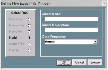
If at any time, you have questions related to the creation or formation of a model, select the menu item Help, which will provide you with context specific assistance. If you explore these help facilities, you will discover not only that they are relatively extensive, but in addition that you can print portions in order to supplement the possi-bly more cursory descriptions in this workbook. Furthermore, as you move from screen to screen, at the top level, if you press the F1 key on your keyboard as you ar-rive at each in turn, an outline description of that screen should immediately appear. In order to begin to create a model, now select the menu item File on the Model Builder and Equation Editor screen, shown in Figure 2. Then click on the line item Create New Model, which is highlighted. In response, a subsidiary window, shown in Figure 3, should then appear. This form obviously allows you to specify the name of a model, its description, and the observation frequency of the data to be used with it. The model name must be between 1 and 8 characters in length, must begin with an alphabetic character, and should contain only alphabetic characters and numbers. For present purposes, the name Klein1 might be appropriate. So enter it. The descrip-tion is opdescrip-tional, but you might wish to put there the words “Klein Model I.” The ob-servation frequency of the model should be specified as Annual, as illustrated. The data for this model, contained in the data bank Kleinbnk, are annual; they span the dates from 1920 to 1941.

Figure 3. Define New Model form

provided any equations. Essentially, we have an empty file, a fact that you need to be aware of, inasmuch as empty files can be confusing to a computer program should you at this point begin to ask the program to display or solve the model. Such files should not be left hanging around your hard drive, lest in the end they confuse you too. It is best to go ahead and start filling this empty box, without further ado.

Figure 4. Model Builder and Editing Screen: New Model Attached

At this point we have several options, for the next step is not rigidly defined. In fact, in terms of the model building process itself, you presently have a number of pos-sible choices, and which of these you should make is in part simply a matter of what you wish to do. For instance, you can begin by entering the model’s identities. Alter-natively, you can estimate the parameters of the behavioral equations then include the identities. Or you can include the various equations in some mixed order. As a piece of software, MODLER does not care which of these options you choose. Furthermore, so far as the ultimate model is concerned, provided that the equations are properly en-tered, each of these choices can lead to the creation of exactly the same model – in terms of its functional properties. The difference will be the initial ordering of its equations, which you may want to evaluate simply in terms of display considerations.

(Save Model As…), or else to rename it or discover its characteristics. Generally, these operations refer to the model broadly and, at the same time, more specifically to various file operations pertaining to the model file.

Next click on the menu item ModelEdit. At this stage, reflecting that the model so far hardly exists, many of the choices are still grayed out. However, observe in par-ticular the three dropdown choices, Add New Equation, Include Another Model’s Equations, and Import Text Equations By Macro. These represent three different ways to enter equations into the model. The first of these, which we will consider presently, provides the means to add equations one at a time. The second provides the means to add one or more equations contained in another MODLER model. Finally, the third allows you to import text equations from any other source, using a text file, generally in the form of a macro file; in this context, such a file can be presumed to contain model equations, which are in effect commands. Of course, these text equa-tions must each obey the MODLER syntactic convenequa-tions for equaequa-tions, and you may therefore need to edit any equations you obtain externally from other software con-texts, among them AREMOS, EViews, MicroFit, PCGive, TROLL, TSP or other such packages. However, in most cases, so long as the package produces text representa-tions of estimated equarepresenta-tions not a lot of editing will be required, inasmuch as other packages commonly implement MODLER’s syntactic conventions.

The one caveat that bears mention is that imported text models can contain redun-dant variables and equations. A common characteristic of other programs is that they may require the creation of extra variables as a prerequisite, in order to express regres-sion and other commands using only variable mnemonic names. MODLER, in con-trast, encourages the embedding of transformations in almost all commands, which as a consequence means that natively created models will normally contain the minimum

number of variables and equations. In particular, MODLER models need not contain identities the sole purpose of which is to define specific transformations. After all, such extra variables do nothing but add to the bookkeeping requirement, as well as to make the models somewhat harder for you to interpret visually. Thus when importing text equations into MODLER, as a prior editing step — using either the inbuilt MODLER text editor or a notes editor such as Notepad or Wordpad — it is generally a good idea to minimize the number of variables by introducing into the imported equa-tions all relevant embedded expressions. Among other benefits, this step will free you later from repeatedly having to update redundant data series that may be nothing more than the sum, log, ratio, or other such transformation of the essential model variables.

Entering New Equations: the Identities

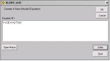
sec-ond is Estimate Equation. Let us begin by adding an identity as the first model equa-tion: if you click on Key In Equation, you will next see a form like that shown in Figure 5. In this figure, the identity has already been inserted, as you can see. Key in this identity yourself, then once you have checked to make sure that you keyed in the same equation as shown here, press the Enter key. By performing these steps, you will have specified the first model equation.

Figure 5. Adding a New Equation

Actually, the fact that you have succeeded in creating a model equation will not be obvious at first, for at this point you will simply be returned to the Model Building and Editing Screen, almost as if nothing has happened. However, if you next select the View menu item, and then click on Complete Model, you will see the screen shown in Figure 6. This display confirms that the model now contains one equation.

Observe two things in particular about this display. First, that the equation will not be displayed until you click successively on View and then Complete Model. Sec-ond, once further equations have been added, the display will not change until you

again click successively on View and Complete Model, or on the relevant icon, which will be quicker. This display does not automatically refresh itself as you change the model. At this stage, you might wish that it did. However, once you get used to MODLER, you would then increasingly find any such automatic display a nui-sance, since it would ultimately slow you down to have to look at everything repeat-edly as you work. Once you have become proficient with the software, you will want to be able to work rapidly, rather than to be forced to look at everything as you go. MODLER is intended to be permissive, rather than dictatorial. It is also intended to be software for people whose time is valuable.

A third aspect is that if you now click also on the File menu item, you will see that no longer are there any grayed out items in this list. A particular option now newly available to you is to copy the display contents to your word processor. Another is to print the display to your printer. These particular display options reflect that an impor-tant aspect of MODLER is the facilities it provides in order to progressively document what you have done at virtually every stage of the process — if you so wish. But do not wish for the moon: you cannot expect the software to display everything automati-cally.

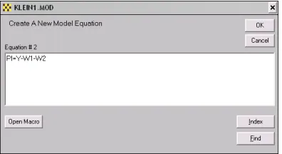
We have created the first equation. In order to add a second identity, choose again the menu item ModelEdit and then Add New Equation. Now, click on Key In Equation and type the next equation, as shown in Figure 7.

Figure 7. Entering the second identity

In-dex, and Find. The first of these will allow you to open a macro—which might con-tain model equations—and, if so, to copy one of these to the blotter of this form sim-ply by double clicking on it. The second, Index, permits you to view the index of any open data bank; for example in case you cannot remember a particular variable name. Similarly, double clicking on an indexed name will move it to the blotter of this form. In turn, Find permits you to make a keyword search of the databank documentation of series, in order to locate variables, either to verify their existence or their names.

Once you have verified your typing of the second identity and have pressed the OK button, you should next see the form shown in Figure 8, which allows you to control where in the model the equation will be put. This particular form did not appear dur-ing the process of enterdur-ing the first model equation, for the obvious reason that locat-ing the equation did not require any human judgment. Here, however, there is some ambiguity, even if only a little. Evidently, you have the choice of putting the new equation either before or after the single, existing model equation. By default, MODLER assumes that you wish to put the equation after, at the end of your model equation(s). Click OK to accept this choice.

Incidentally, it is generally a bad idea to use this form to attempt to locate model equations at “future” locations, such as 3,4,5, or 6. At the moment, the model has only 2 equations and you can confuse both MODLER and yourself if you attempt to ma-nipulate and display a model that contains separated equations interspersed with blank placeholders. Generally, the program only “knows” the number of equations in a model from the highest number equation inserted; it has no way of determining that a blank equation is simply a place holder and will attempt to print blank equations as well as given equations. In addition, as you add further equations, MODLER will tend to increment the number of model equations even if the last added equation is placed in a previously “blank” location within the range of model equations. Furthermore, until you are an experienced user of the program, you are likely to find it difficult, af-ter the fact, to delete “blank” equations.

The final identity of the model is K=I+K(-1). If you repeat the last step, but this time enter this capital stock identity into the form shown in Figure 7, instead of the prior one, and then click OK, you will be shown once again the form displayed in Fig-ure 8; the default this time will be to add the final identity as equation number 3. To do this, simply click OK.

We have now created a three-equation model, consisting entirely of identities. At this point, if you once again click on the View menu item and then Complete Model, you should then see the model display shown in Figure 9. Notice in passing that the mnemonics shown immediately after each equation number — Y, PI, and K, respec-tively — specify the equation variable that that equation “explains” and therefore on which that equation is “normalized.” We will consider this aspect of the model dis-play in more detail later.

However, before we move on, notice also one other thing, which is that, so far, we have not needed to use any data. The identities have been added to the model simply as coded equations, without any need to retrieve observations from a data bank or other data source.

Figure 9. Identities for Klein Model I

Estimating the Behavioral Equations

the model, in the location you choose, either explicitly or by default. Simultaneously, it also creates a machine language analogue of the equations, and performs various be-hind-the-scenes housekeeping chores. Inasmuch as these operations are performed no matter how complex the estimated equation, this is a MODLER feature that required a substantial amount of time to design and code, notwithstanding that it is now per-formed daily in nanoseconds. It is an operation that is not analytically perper-formed by any other existing econometric software package.

The estimation of equation parameters is invoked by clicking again on ModelEdit, then Add Equation. However, this time choose Estimate Equation, rather than Key In Equation. Immediately, your screen should look much like the display shown in Figure 10. Notice, in the center of the screen, the form entitled Edit/Execute Com-mand, which is superimposed on the form labeled Parameter Estimation, which is it-self superimposed on the Model Builder & Equation Editor screen. Focus first on this Edit/Execute form. Should you be unfamiliar with the syntactical conventions of MODLER regression commands, press its Help button for information, including de-scriptions of the logical, relational, and mathematical operators and statistical func-tions that can be used in regression commands, either on their own or in combination. Notice also that you can directly open a macro from this form, by pressing the Open Macro button, should you wish to copy a regression command, whole or in part, that is contained in some macro file. The Index and Find buttons can be used to discover the names of databank variables that you might imperfectly remember. All these facilities are likely to be familiar from your earlier use of MODLER; the important point is that all these options are also immediately available at this stage.

Type into the Edit/Execute Command Form the regression command:

CE=f(W1+W2,PI,PI(-1))

If you should make a mistake, you can of course use the normal text editing facilities in this context, invoked by a click of your right mouse button, including the ability to cut, copy, and paste. Unless you have changed standard MODLER defaults, any vari-able names or other text typed into this command form will be case insensitive, so that it does not matter whether or not you capitalize what you type. But be sure to include the double parentheses at the end of the command, or else MODLER will tell you that your parentheses do not match; in that case it will also provide you the ability to cor-rect this error.

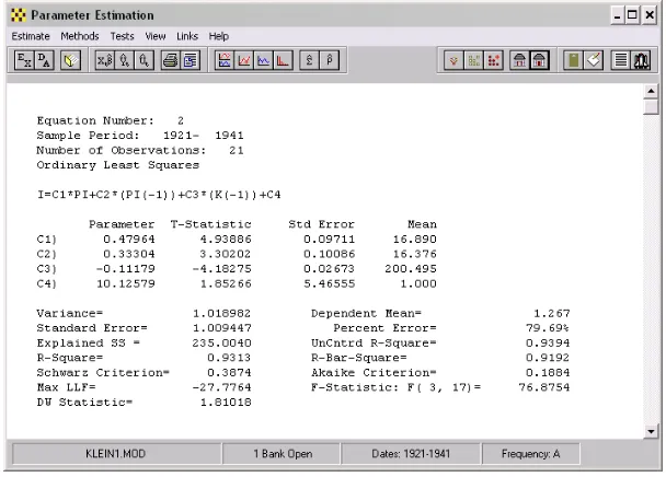
When you have correctly entered the regression command and pressed the OK but-ton, you should immediately see the parameter estimation screen displayed in Figure 11. Observe that the estimated parameter values are not exactly those given earlier, reflecting that here they have been estimated using Ordinary Least Squares, rather than maximum likelihood [19, p. 67-68], however they do match the OLS estimates given by Klein (Page 75), as well as in Berndt and other relevant texts [4, Chapter 10]. As a separate exercise, you can compute a variety of different estimates, if you wish. For example, as mentioned earlier, the macro files that complement this workbook also in-clude one that permits you to compute Two Stage Least Squares estimates, and with some work you can also compute the maximum likelihood estimates calculated by Klein. These options will be considered in a later chapter.

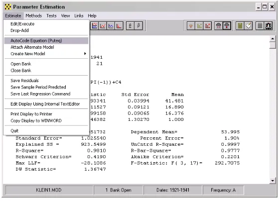
Considering the Parameter Estimation screen shown in Figure 11, notice, in particu-lar, that there are many supplementary options available to you at this point. For in-stance, you can view graphs of actuals and predicted, and/or the regression residuals. As just indicated, you can select alternative estimation methods, instead of the default Ordinary Least Squares. You can in addition capture this regression display and save it as a file, copy it to your word processor, or print it on your printer. Or you can copy it to the clipboard. The general MODLER User Guide provides a more detailed de-scription of all these various options. Our interests at the moment are specific: please select Estimate on the menu bar. You should then immediately see the dropdown list shown at the left of Figure 12.

Figure 12. AutoCoding and Other Options

Focusing on the dropdown list, look specifically at the third item, AutoCode Equa-tion (Puteq), which is highlighted in the figure. If you click on this item, one of two things will occur. First, you may see the form displayed in Figure 13, which is called a Destination Form. Alternatively, you may see an error message telling you that the program cannot find the regression results.

“know” that it has everything it needs to have. Autocoding is a complex operation, as noted earlier, so that if you have displayed one or more regression graphs, or looked at something else to do with the regression results, MODLER is programmed to check to make sure that absolutely nothing has occurred simultaneously that will adversely af-fect the autocoding operation. Actually, here, MODLER is programmed to err on the safe side: if anything might have occurred, MODLER will issue this error message. However, in this event, there is a simple solution: it is to re-select Estimate and then click on Edit/Execute, to re-estimate the equation. Once the regression results have been re-displayed, click once more on AutoCode Equation (Puteq); this time you should see the form displayed in Figure 13.

Figure 13. AutoCode Equation: Location of Model Equations

It should be immediately evident from Figure 13 that estimated equations that are Autocoded and inserted into a model are, by default, appended as the last model equa-tion. Moreover, by default, they are loaded into the currently attached model. How-ever, you can also see from Figure 13 both that estimated equations can be used not only to replace existing model equations, but instead can be put into some other, speci-fied model. When you are estimating a model the first time, most of these choices are superfluous; however, if you re-estimate, or if you later wish to create alternative ver-sions of a model, they may not be.

individual variable it is said to be normalized on. This process can include inverting the equation so that a variable formerly on the right-hand-side occurs on the left-hand-side as the dependent variable. In all cases, equations can only be normalized on con-temporaneous variables: inasmuch as lagged variables represent the past and lead vari-ables the future, generally only contemporaneous varivari-ables can be “explained” by a given model equation.

Notice also that the Inspect button permits you to “inspect” the model before the current estimated equation is added. If this button is enabled and is pressed, the Model Building & Editing screen becomes the active “window,” thus allowing you to view model equations, variables, and other properties of the model. You can, for ex-ample, verify that the equation you are about to add is not already represented in the model or, if it is, determine its equation number, so that you can replace the existing version with the just-estimated equation. However, there are instances (such as at present) in which the Model Building & Editing screen is already displayed on your desktop, although momentarily it may be behind another screen. In this case, either the Inspect button may be disabled or, if it is enabled, and you press it, MODLER may display an error message to the effect “Model Building & Editing Screen Already Dis-played. Select Status Bar Icon.” You can make this screen active simply by clicking on the appropriate desktop status bar icon; it is not necessary to display another copy of this screen.

Finally, observe the Browse button on the Destination Form shown in Figure 13. It is there to allow you to browse your hard disk or other storage device in order to de-termine the location of some other model into which you could “put” the current esti-mated equation. Bear in mind that whereas a model file is presumed to be a container for a “model,” there is no reason why you cannot create one or more “extra” MOD files, should you wish, simply to use as repositories for sets of estimated equations. There is obviously no requirement that any given MOD file must at some point be used to hold a solvable model. Recall the earlier, brief discussion of the MODLER command that permits one or more equations to be copied from one MODLER-created model to another: it is perfectly permissible to use a given MOD file to hold any num-ber (up to 1000) of alternative versions of an equation, and then at the end to copy your final choice from among them to another MOD file that then will be used as a “true” model file.

Figure 14. Regression Command for Net Investment Equation

Recall that the text box (blotter) of this form permits you to edit its contents, should you make a mistake: to accomplish this, click on your right mouse button while point-ing at this blotter and the standard editpoint-ing options floatpoint-ing menu will appear. This fea-ture is a MODLER capability in combination with Windows, generally requiring Win-dows 98 or later. However, provided this operating system criterion is met, it is a standard feature of MODLER: in almost every instance that you are called upon to in-sert text, you are able to edit, cut, copy, and paste.

Notice also that the form in Figure 14 exhibits a set of buttons, including in particu-lar the Help, Open Macro, Index, and Find buttons. The first provides context spe-cific help that describes the conventions, syntax, and options for regression commands specifically, including the set of operators and implicit functions that can be used. The Open Macro button permits you to open any macro, and if you highlight any part of its contents, to copy this highlighted text automatically. Double clicking on any line’s contents will capture that line of macro text. For example, you can use this button to extract a regression command contained in that macro; of course, this operation leaves the macro undisturbed. As always, the Index and Find buttons permit you to discover the names and characteristics of variables in any open data bank or Memory File. These buttons are described in much greater detail in the MODLER User Guide; they are mentioned here once more just to remind you of their utility when building a model.

Now that you have entered this Investment equation, and verified that it is correct, click OK. Make sure, before clicking OK, that you have entered the ending, right double parentheses, as shown. If you omit one or both of these, MODLER will issue an error message to the effect that “parentheses do not match,” and then allow you to correct this error.

The essential difference is that here the parameters are shown symbolically (C1, C2, … , CN). The rows just below this equation display, beginning with these symbols as labels, present the parameter estimates and related statistics.

Figure 15. Estimated Net Investment Equation

Once you have verified your results, then successively select the menu item Esti-mate and its dropdown element AutoCode (Puteq). You will at this stage once again see a Destination form similar to that shown in Figure 13 above. Click OK in order to insert the estimated version of this equation into the model. If you accept the default, this operation will have the effect of appending this equation to the model. The model should now contain 5 equations: three identities and two estimated equations.

dis-cover that you optionally have a great deal of control over the particular test statistics that are shown and their characteristics, as well as various additional test facilities, in-cluding Unit Root and related cointegration tests. These are not discussed here for the simple reason that the purpose of the present description is to describe how to form a model using the Klein Model I as a template. However, were you to use MODLER to create your own model, then these test statistics would be quite relevant and you would want to use them in order to make choices concerning which form of each equa-tion you might wish to add to your model. Obviously, on your own you can consider all these tests in conjunction with the Klein model results; a recent book considers as-pects of these statistics and their presentation [30].

If you also then click on the View menu item shown in Figure 15, you will then see the drop down menu shown in Figure 16. Among the options available are those that can be accessed by clicking on Model Equation(s) and Other Model Elements. Your display may look slightly different, because of a double row of icon buttons, but will be essentially the same in function.

Figure 16. "View" Related Facilities

far either keyed in or estimated. Alternatively, if you choose Other Model Ele-ments, the Model Builder & Editor screen will be displayed, allowing you, if you wish, to examine the model in detail.

Figure 17. Model Equations

1921, … and the explicit statement of the model might be marginally more readable. Of course, the variable could also be called TIME, rather than T.

Figure 18. Private Wage Equation Regression Command

Click OK to obtain the results shown in Figure 19 then select Estimate, AutoCode (Puteq), and again click OK on the Destination form, in order to insert the estimated version of this equation into the model.

One aspect of the equation displayed in Figure 19 that should be noted particularly is the inclusion of the expression Y+TAX-W2, in both contemporaneous and lagged form. Obviously, the ability to embed such expressions has the effect of making the estimated equation more instantly readable—as opposed to if this expression were to be replaced by a variable called XXX, or some other mnemonic name. However, as discussed previously, the fundamental virtue of being able to embed expressions di-rectly is that this MODLER capability permits the model to be parsimoniously stated in its entirety, which is more than a matter of simple elegance. Extra variables essen-tially require extra definitional identities that litter the model and take up space in the model databank. More importantly, as a conceptual matter, they also make the model more difficult to read and understand. At the beginning of the next chapter, we will see in Figure 20 that MODLER’s text presentation of the model is virtually identical to what might be published in a book describing the model, without requiring any spe-cific editing. A fundamental reason is the software’s automatic ability to interpret ex-pressions within commands, as well as to display them.

A lot more could be said about the estimation process, especially in terms of the documentation of the model as a nearly automatic by-product. For example, at each stage, it is possible to capture the estimated equation display. As a general software feature, this display can be printed on your printer, copied to the clipboard, or directly transferred to your word processor, assuming of course that when you originally set up MODLER, you established all the proper settings, as described in the MODLER Get-ting Started Guide. The purpose of capturing the results at each stage might be to pro-duce full documentation of each step of the model building process, either for record keeping or publication.

As you have been reading this workbook you have actually been watching this documentation occur, the only difference being that screens have been displayed here for the purpose of illustrating how your monitor will look at each step, rather than pre-senting the results in the form of text and graphics suitable for publication as a book or report. The presentation here has also subsumed other self-documenting MODLER features. For example, the Standard Index to the KLEINBNK data bank, when printed on your printer, or copied to your word processor, becomes in effect a glossary of model variables. Of course, the usefulness of such a glossary always depends on the person who creates and maintains the model databank, upon that person’s willingness to describe the variables well.

Chapter 2 Forming the Model

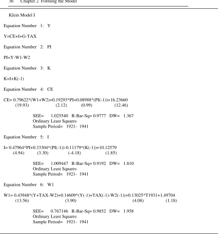
The model estimated in the first chapter is displayed below in Figure 20. The crea-tion of this model, as described in the last chapter, involved estimating its unknown parameter values using Ordinary Least Squares. As was noted there, this method is not the only possible choice: the parameters could instead have been estimated in any of a variety of ways, including Two Stage Least Squares or Three Stage Least Squares, as well as Limited Information Maximum Likelihood, among other methods. Fur-thermore, the implications will not be the same: the particular estimation method used affects the specific parameter estimate values obtained and also the stochastic proper-ties of the resulting model when it is solved. A useful supplementary and amplifying discussion is provided by Berndt [4], who considers the various methods that have been used by economists over the years to estimate Klein Model I, pulling together and referencing a number of previous studies. After considering the alternatives, it is possible, should you wish, to replicate at least certain of these methods using MODLER, either now or later. Furthermore, if you are willing to take the trouble to key in all the values, it is perfectly possible to form the model in the context of MODLER using any parameter estimates you have access to, not just those that can be produced by the program.

Figure 20. Complete Klein Model I

Klein Model I

Equation Number 1: Y

Y=CE+I+G-TAX

Equation Number 2: PI

PI=Y-W1-W2

Equation Number 3: K

K=I+K(-1)

Equation Number 4: CE

CE= 0.79622*(W1+W2)+0.19293*PI+0.08988*(PI(-1))+16.23660 (19.93) (2.12) (0.99) (12.46)

SEE= 1.025540 R-Bar-Sq= 0.9777 DW= 1.367 Ordinary Least Squares

Sample Period= 1921- 1941

Equation Number 5: I

I= 0.47964*PI+0.33304*(PI(-1))-0.11179*(K(-1))+10.12579 (4.94) (3.30) (-4.18) (1.85)

SEE= 1.009447 R-Bar-Sq= 0.9192 DW= 1.810 Ordinary Least Squares

Sample Period= 1921- 1941

Equation Number 6: W1

W1= 0.43948*(Y+TAX-W2)+0.14609*(Y(-1)+TAX(-1)-W2(-1))+0.13025*T1931+1.49704 (13.56) (3.90) (4.08) (1.18)

SEE= 0.767146 R-Bar-Sq= 0.9852 DW= 1.958 Ordinary Least Squares

Further Elaboration of the Model

As just indicated, a model can be estimated using only linear parameter estimation methods, yet be a highly nonlinear system, once formed as a working model. Con-versely, it is at least conceivable that a model could be estimated using non-linear es-timation procedures, yet be a linear model when considered as a set of equations. However, before addressing these several models-as-sets-of-equations issues, it is use-ful to talk first about the inferences you can draw from the way in which models are displayed. Consider Figure 20 simply as a display. Observe that the behavioral equa-tions are shown with a standard set of supporting statistics; this figure exactly repli-cates MODLER’s standard model display. Furthermore, you need to be aware that, within MODLER, such statistics will be displayed for any particular equation only so long as you do not subsequently edit that equation, in the process changing its proper-ties. Of course, this particular display, as you view it, has been copied to a word proc-essing document and there it could of course have been changed without necessarily causing the associated statistics to vanish, but when considering such a model display entirely within MODLER, you have some assurance that you will know whether each equation is displayed as originally estimated. In particular, if supporting statistics are not present you know that the equation was not estimated and autocoded by MODLER — or that it has been changed in some essential way since estimation; as prosaic as this facility may initially seem, it is nevertheless a model validation feature.

Notice also that, for each equation, the mnemonic for the variable that is “ex-plained” by that equation is shown immediately to the right of the equation number, as very briefly indicated earlier. It is characteristic of this type of MODLER display that the autocoded behavioral equations will always be shown in the form they were esti-mated. Thus, after the fact, you can always discover the estimation specification. However, what is also implied is that if the equation has subsequently been normalized or later re-normalized, this normalization will be indicated by the mnemonic that ap-pears immediately after the equation number for each equation. This subtlety has the possible defect that, for a normalized equation, you are not shown the specific normal-ized form. The saving grace is that MODLER normalizes equations analytically, so that the normalization is unique; therefore, you are always able to derive it yourself if you wish. Actually, across software packages, there has never been an agreed standard established for such equation displays — only one or perhaps two other packages have ever permitted normalization, and then using nonanalytic methods, generally involving an initial linearization by Taylor’s expansion, or by first requiring you to specify the normalization formulae manually.

few exceptions to this rule and certain specific restrictions in the case of a model—for instance, statistical functions such as MEAN, SDEV, and others defined on the do-main of a particular estimation sample date range—cannot be used in models, for the obvious reason that in the context of a model solution, these are scalar constants and should be so represented. However, in general, you are able to form regression and other commands that are stated in terms of the basic model variables. As a result, models created by MODLER are easily understood, inasmuch as extraneous identities are therefore unnecessary. Furthermore, among the other implications is that usable models can be formed very quickly. The model shown in Figure 20 is ready to be solved, fresh from estimation — that is, if you wish to proceed directly, only three commands stand between it and its first sample solution.

However, the fact that MODLER permits an elegant statement of a model does not

mean that parsimony is required. At a later stage, when you begin to create tables, graphs, and other such displays, in order to present model solution results, you may wish to create additional model variables specifically for display purposes. For in-stance, you may wish to monitor relationships between specific variables, for example in the form of ratios [20], even though these constructs play no specific part in the formulation of your model. In the case of Klein Model I, simple as it is, there are various ways to elaborate the model. For example, as Berndt implicitly points out [4, p. 551], this model inherently subsumes several potentially interesting additional iden-tities, even if these are formally redundant. In particular, define Total Wages, W, as:

W= W1 + W2

and Income, Y, as:

Y = PI + W

Total Product can then be stated as:

Y + TAX = CE + I + G

and Private Product, E, as:

E = Y + TAX – W2

You will recognize each of these as having a role in the model.