Schechter Function Model for the QSO Luminosity Function from the SDSS DR7

http://dx.doi.org/10.4236/ijaa.2016.63020

How to cite this paper: Singh, S.A., Meitei, I.A. and Singh, K.Y. (2016) Schechter Function Model for the QSO Luminosity Function from the SDSS DR7. International Journal of Astronomy and Astrophysics, 6, 247-253.

http://dx.doi.org/10.4236/ijaa.2016.63020

Schechter Function Model for the QSO

Luminosity Function from the SDSS DR7

Salam Ajitkumar Singh

_{, I. Ablu Meitei}

_{, K. Yugindro Singh}

1_{Department of Physics, Manipur University, Imphal, India} 2_{Department of Physics, Modern College, Imphal, India}

Received 5 July 2016; accepted 8 August 2016; published 11 August 2016

Copyright © 2016 by authors and Scientific Research Publishing Inc.

This work is licensed under the Creative Commons Attribution International License (CC BY). http://creativecommons.org/licenses/by/4.0/

Abstract

A study of the optical luminosity function of Quasi Stellar Objects (QSOs) and its evolution with redshift is carried out using the data from the Sloan Digital Sky Survey Data Release Seven (SDSS DR7). It is shown that the observed QSO luminosity function is well fitted by a Schechter function model of the form

( )

(

)

(

) (

)

∗ ∗ ∗ ∗

Φ = Φ α − , where Li

∗ _{is the break or}

charac-teristic luminosity with luminosity evolution characterized by a second order polynomial in red shift. The best fit parameters are determined by using the Levenberg-Marquardt method of nonli-near least square fit.

Keywords

Galaxies: Active, Quasars: General, Galaxies: Luminosity Function

1. Introduction

Quasi Stellar Objects (QSOs) or quasars were defined originally as star-like objects of large redshift. They are powered by the accretion of matter onto supermassive black holes (SMBHs). The QSOs are considered to be the most luminous subclass of Active Galactic Nuclei (AGNs) [1]. Soon after the discovery of QSO [2], their popu-lation was observed to evolve strongly with redshift. As a result these objects provide a unique tool in the study of galaxies and large-scale structure formation throughout the history of the universe [3]. The QSO luminosity function and its evolution with redshift provide important clues about the demographics of the AGN population and strong constraints on physical models and evolutionary theories of AGN [4]-[6]. The faint-end slope of the luminosity function is a measure of how much time QSOs spend at relatively low accretion rates. On the other

*

hand, the bright-end slope tells us about the intrinsic properties of the QSO population during the time when black holes were increasing in mass most rapidly (e.g. triggering rate, active black mass function, etc.) [7].

The differential QSO luminosity function is defined as the number density of QSOs per unit comoving vo-lume, and per unit luminosity as a function of luminosity and redshift [8] [9]. The luminosity function is usually derived by using the 1V_max method (e.g. [10]-[14]). The most common analytical representation for the shape of the QSO luminosity function in the literature is a double power-law (e.g. [6] [15]-[22]). In this paper, we use the Schechter function model [23] to describe the shape of the QSO luminosity function. In earlier papers such as Goldschmidt et al. (1998) [24], Warren et al. (1994) [25] and Singh et al. (2016) [26] the Schechter function is found to represent the shape of the QSO luminosity function. Using the Edinburgh UVX quasar survey, Goldschmidt et al. (1998) [24] used the Schechter function model with the evolution of the characteristic mag-nitude, M*

( )

γ

(

)

The fit is observed to be acceptable with a significance level for rejection of 10%. Warren et al. (1994) [25] used the Schechter function model with evolution of the characteristic magnitude of the form M*

( )

τ

usinga wide-field multicolor survey for high redshift quasars (z≥ 2.2), where τ is the look-back time. Singh et al. (2016) [26] has shown that the shape of the QSO luminosity functions is adequately represented by the Schech-ter function with second order polynomial evolution model from the 2QZ and 6QZ samples in the redshift range 0.3 ≤ z≤ 2.4.

Historically, there are two fundamental models for the evolution of QSOs namely, pure luminosity evolution (PLE) and pure density evolution (PDE). If the redshift and luminosity dependence are separable, the evolution of the luminosity function can be modelled in terms of the PLE where QSO luminosities change with time, but the total number of QSO remains constant and the PDE where the number density of QSOs changes but their luminosities remain constant. Various hybrid models such as luminosity and density evolution model (LEDE) and luminosity-dependent density evolution model (LDDE) are also used to describe the evolution of QSOs with redshift. Ross et al. (2013) [21] and Croom et al. (2009) [7] presented the luminosity function evolved with LEDE where the bright-end and faint-end slopes have fixed values and normalization and characteristic lumi-nosity evolve independently. Croom et al. (2009) [7] and Bongiorno et al. (2007) [27] used the LDDE to study the luminosity evolution of QSOs. The luminosity evolution of QSOs with redshift in this paper is described by the PLE.

In section 2 we give a brief description of the SDSS sample. The determination of the binned optical luminos-ity function and its evolutionary behaviors are presented in section 3. Finally in section 4 we give our conclusion. Throughout this paper we use a Ʌ cosmology with Ω =m 0.3, Ω =Λ 0.7, and Ho= 70.0 km⋅s−1⋅Mpc−1.

2. The Sample

The Sloan Digital Sky Survey Data Release Seven (SDSS DR7) [28] uses a CCD camera [29] on a dedicated 2.5 m wide field telescope [30] located at Apache Point Observatory (APO) near the Sacramento peak in Southern New Mexico, to obtain images in five photometric bands: u, g, r, i and z [29] [31] over approximately 10,000 square degrees of high Galactic latitude sky in the Northern Hemisphere [32]. The survey data-processing soft-ware measures the properties of each detected object in the imaging data in all five photometric bands and de-termines and applies both astrometric and photometric calibrations [33]-[35]. The photometricis calibrated to an AB system [36] and the photometric measurements are reported as asinh magnitudes [37]. The spectroscopy is performed by using a 640-fibre-fed pair of multiobject double spectrographs with coverage from 3800 Å to 9200 Å and a resolution of λ λ∆ of roughly 2000 [28].

The final SDSS DR7 quasars catalog from SDSS I/II was presented in Schneider et al. (2010) [38] which contains 105,783 spectroscopically confirmed quasars and the redshift distribution of these QSOs is also shown in Singh et al. (2014) [39]. The catalog consists of quasars that have a luminosity larger than Mi = −22.5

(calcu-lated assuming Ʌ cosmology with Ω =m 0.3, Ω =Λ 0.7, and Ho = 70.0 km⋅s−1⋅Mpc−1) and have at least one

3. The Luminosity Function and Its Analysis

The optical luminosity function of QSOs is determined by using the 1V_max method [42]. It is given by

[

]

(

)

_[

_]

max,

1 1

2

2

N

i

j

i j

M z

M z V

 

Φ = = _ _

∆ =

∑

with a Poisson statistical uncertainty

( )

_[

_]

1 2 2

max,

1 1

, 2

N

j

i V j

M z

σ Φ =  _ _ 

=  _{ } 

 

∆

∑

where V_max,j is the volume corresponding to the maximum distance that object j could be observed, and still be included in the sample. The summation is over all quasars within a redshift-magnitude bin.

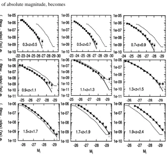
Figure 1 shows the binned optical luminosity function of QSOs (indicated by filled circle points) for nine redshift intervals i.e. 0.3 ≤ 0.5; 0.5 ≤ z≤ 0.7; 0.7 ≤ z≤ 0.9; 0.9 ≤ z≤ 1.1; 1.1 ≤ z≤ 1.3; 1.3 ≤ z≤ 1.5; 1.5 ≤ z≤ 1.7;

1.7 ≤ z ≤ 1.9 and 1.9 ≤ z≤ 2.4. The bin size of absolute magnitude, ∆M_i is 0.3 mag.

The shape of the QSO luminosity function is fitted by the Schechter function model [23]. The generalized form of the Schechter function model is given by

( )

* exp * *

i i i

i i

i i i

L L L

L dL d

L L L

α

     

Φ = Φ _{  }− _{  }

     

which, in terms of absolute magnitude, becomes

Figure1. The binned optical luminosity functions of QSOs for the SDSS DR7 sample

Table 1.The best fitting parameter values derived from the SDSS DR7 sample for the Schechter function model with second order polynomial in redshift.

Redshift ranges α *

i

M k1 k2

* 6

10

φ _× − (Mpc−3⋅mag−1)

2

v

χ

1.5 - 2.4 −2.52 −22.96 1.91 −0.44 0.09 40.48/28

0.3 - 1.5 −2.32 −23.99 1.46 −0.35 0.13 298.50/76

0.3 - 2.4 −2.32 −23.97 1.38 −0.30 0.15 412.43/109

( )

( )

(

)

(

)

*

0.4 10 10 Mi Mi exp 10 Mi Mi

i

M In α

φ = φ − − + × _− − − _

  (3)

where φ* _{is a normalization parameter whose dimension is the number density of objects,} α _{is the faint-end}

slope of the luminosity function and *

i

L is the characteristic luminosity (with an equivalent characteristic abso-lute magnitude, *

i

M ). The evolution of the luminosity function is described by the redshift dependence of the characteristic luminosity or magnitude. We have modelled this evolution as a second-order polynomial in red-shift of the form

( )

( )

1 2

* * _{0 10}k z k z

i i

L z =L +

or in terms of absolute magnitude,

( )

( )

(

)

* * 2

1 2

0 2.5

i i

M z =M − k z+k z (4)

By using equations (3) and (4), we fit the PLE model to the binned optical luminosity function determined by Shen & Kelly (2012) [41] in various redshift ranges. The best-fitting parameters are determined from the PLE model by using the Levenberg-Marquardt method of nonlinear least square fit [43]. The resulting best-fitting parameters in various redshift ranges are listed in Table 1. In Figure 1, the solid lines represent the Schechter function model with PLE fit to the observed luminosity functions of QSOs. In assessing the goodness-of-fit, we measure the χ2 _{value by comparing the observed luminosity function and theoretical luminosity function}

pre-dicted by best fit model. A χ2 _{comparison of the model luminosity function to the binned luminosity function}

gives χ2 _v=_{412.43 109 for 0.3} ≤ _z≤ 2.4. But, if we restrict the redshift range being fit, we obtain significant

improvement with χ2 _v=_{40.48 28 for the redshift range 1.5} ≤ _z≤ 2.4. Thus, the Schechter function model

can be regarded as simply one way of describing the basic shape of the QSO luminosity function which displays a steepening above the characteristic luminosity *

i

L (or below a characteristic absolute magnitude *

i

M ). From Figure 1, it is clear that there is in general good agreement between the model and data. However, there are more bright QSOs than predicted by the model at the bright end of the luminosity function which is due to the exponential decrease in the Schechter function model at *

i i L >L .

4. Conclusion

The shape of the luminosity function of QSOs and its evolution with redshift are studied by using the Schechter function model with PLE. The best fitting parameter values for the model are determined by using the Leven-berg-Marquardt method of nonlinear least square fit. For the Schechter function model the dimensionless para-meter α gives the slope of the luminosity function for QSOs fainter than the characteristic luminosity *

i L (i.e.

*

i i

L L ); for QSOs more luminous than the characteristic luminosity *

i

L (i.e. *

i i

L L ), the luminosity func-tion drops exponentially with luminosity. A comparison of the χ2 _{values and the number of degrees of}

free-dom shows that the Schechter function model with polynomial evolution of the characteristic magnitude pro-vides acceptable fit to the QSO luminosity function.

Acknowledgements

Funding Council for England. The SDSS Web site is http://www.sdss.org/.

One of the authors (Salam Ajitkumar Singh) is grateful to the Indian Space Research Organization, Department of Space, Government of India for providing JRF under a RESPOND Project (ISRO/RES/2/385/2013-14).

References

[1] Osmer, P. (2006) Quasistellar Objects: Overview from Encyclopedia of Astronomy and Astrophysics. IOP Publishing Ltd., London.

[2] Schmidt, M. (1963) 3C 273: A Star-Like Object with Large Red-Shift. Nature, 197, 1040.

http://dx.doi.org/10.1038/1971040a0

[3] Kennefick, J.D., Djorgovski, S.G. and De Carvalho, R.R. (1995) The Luminosity Function of z>4 Quasars from the Second Palomar Sky Survey. The Astronomical Journal, 110, 2553. http://dx.doi.org/10.1086/117711

[4] Haehnelt, M.G. and Rees, M.J. (1993) The Formation of Nuclei in Newly Formed Galaxies and the Evolution of the Quasar Population. Monthly Notices of the Royal Astronomical Society, 263, 168-178.

http://dx.doi.org/10.1093/mnras/263.1.168

[5] Terlevich, R.J. and Boyle, B.J. (1993) Young Ellipticals at High Redshift. Monthly Notices of the Royal Astronomical Society, 262, 491-498. http://dx.doi.org/10.1093/mnras/262.2.491

[6] Boyle, B.J., Shanks, T., Croom, S.M., et al. (2000) The 2dF QSO Redshift Survey-I. The Optical Luminosity Function of Quasi-Stellar Objects. Monthly Notices of the Royal Astronomical Society, 317, 1014-1022.

http://dx.doi.org/10.1046/j.1365-8711.2000.03730.x

[7] Croom, S.M., Richards, G.T., Shanks, T., et al. (2009) The 2dF-SDSSLRG and QSO Survey: The QSO Luminosity Function at 0.3< <z 2.4. Monthly Notices of the Royal Astronomical Society, 399, 1755-1772.

http://dx.doi.org/10.1111/j.1365-2966.2009.15398.x

[8] Fan, X., Strauss, M.A., Schneider, D.P., et al. (2001) High-Redshift Quasars Found in Sloan Digital Sky Survey Com-missioning Data. IV. Luminosity Function from the Fall Equatorial Stripe Sample. The Astronomical Journal, 121, 54-65. http://dx.doi.org/10.1086/318033

[9] Jiang, L., Fan, X., Cool, R.J., et al. (2006) A Spectroscopic Survey of Faint Quasars in the SDSS Deep Stripe. I. Pre-liminary Results from the Co-Added Catalog. The Astronomical Journal, 131, 2788-2800.

http://dx.doi.org/10.1086/503745

[10] Richards, G.T., Strauss, M.A., Fan, X., et al. (2006) The Sloan Digital Sky Survey Quasar Survey: Quasar Luminosity Function from Data Release 3. The Astronomical Journal, 131, 2766-2787. http://dx.doi.org/10.1086/503559

[11] Greene, J.E. and Ho, L.C. (2007) The Mass Function of Active Black Holes in Local Universe. The Astrophysical Journal, 667, 131-148. http://dx.doi.org/10.1086/520497

[12] Vestergaard, M., Fan, X., Tremonti, C.A., Osmer, P.S. and Richards, G.T. (2008) Mass Functions of the Active Black Holes in Distant Quasars from the Sloan Digital Sky Survey Data Release 3. The Astrophysical Journal, 674, L1-L4.

http://dx.doi.org/10.1086/528981

[13] Vestergaard, M. and Osmer, P.S. (2009) Mass Functions of the Active Black Holes in Distant Quasars from the Large Bright Quasar Survey, the Bright Quasar Survey, and the Color-Selected Sample of the SDSS Fall Equatorial Stripe.

The Astrophysical Journal, 699, 800-816. http://dx.doi.org/10.1088/0004-637X/699/1/800

[14] Schulze, A. and Wisotzki, L. (2010) Low Redshift AGN in the Hamburg/ESO Survey II. The Active Black Hole Mass Function and the Distribution Function of Eddington Ratios. Astronomy &Astrophysics, 516, A87.

http://dx.doi.org/10.1051/0004-6361/201014193

[15] Pei, Y.C. (1995) The Luminosity Function of Quasars. The Astrophysical Journal, 438, 623-631.

http://dx.doi.org/10.1086/175105

[16] Boyle, B.J., Shanks, T. and Peterson, B.A. (1988) The Evolution of Optically Selected QSOs-II. Monthly Notices of the Royal Astronomical Society, 235, 935-948. http://dx.doi.org/10.1093/mnras/235.3.935

[17] Croom, S.M., Smith, R.J., Boyle, B.J., et al. (2004) The 2dF QSO Redshift Survey—XII. The Spectroscopic Catalogue and Luminosity Function. Monthly Notices of the Royal Astronomical Society, 349, 1397-1418.

http://dx.doi.org/10.1111/j.1365-2966.2004.07619.x

[18] Richards, G.T., Croom, S.M., Anderson, S.F., et al. (2005) The 2dF-SDSS LRG and QSO (2SLAQ) Survey: The z < 2.1 Quasar Luminosity Function from 5645 Quasars to g = 21.85. Monthly Notices of the Royal Astronomical Society,

360, 839-852. http://dx.doi.org/10.1111/j.1365-2966.2005.09096.x

[19] Glikman, E., Bogosavljević, M., Djorgovski, S.G., et al. (2010) The Faint End of the Quasar Luminosity Function at z

[20] Glikman, E., Djorgovski, S.G., Stern, D., et al. (2011) The Faint End of the Quasar Luminosity Function at z ~ 4: Im-plications for Ionization of the Intergalactic Medium and Cosmic Downsizing. The Astrophysical Journal Letters, 728, L26. http://dx.doi.org/10.1088/2041-8205/728/2/L26

[21] Ross, N.P., McGreer, I.D., White, M., et al. (2013) The SDSS-III Baryon Oscillation Spectroscopic Survey: The Qua-sar Luminosity Function from Data Release Nine. The Astrophysical Journal, 773, 14.

http://dx.doi.org/10.1088/0004-637X/773/1/14

[22] Singh, I.A. and Singh, K.Y. (2013) The Evolution QSOs—The Optical Luminosity Function. International Journal of Astronomy and Astrophysics, 3, 87-92. http://dx.doi.org/10.4236/ijaa.2013.32009

[23] Schechter, P. (1976) An Analytic Expression for the Luminosity Function for Galaxies. The Astrophysical Journal, 203, 297-306. http://dx.doi.org/10.1086/154079

[24] Goldschmidt, P. and Miller, L. (1998) The UVX Quasar Optical Luminosity Function and Its Evolution. Monthly No-tices of the Royal Astronomical Society, 293, 107-112. http://dx.doi.org/10.1046/j.1365-8711.1998.01131.x

[25] Warren, S.J., Hewett, P.C. and Osmer, P.S. (1994) A Wide-Field Multicolor Survey for High-Redshift Quasars z≥ 2.2.

III. The Luminosity Function. The Astrophysical Journal, 421, 412-433. http://dx.doi.org/10.1086/173660

[26] Singh, S.A. and Singh, K.Y. (2016) The QSOs Luminosity Function from the 2dF QSO Redshift Survey and the Asso-ciated 6dF QSO Redshift Survey at 0.3≤ ≤z 2.4. Advances in Astrophysics, 1, 106-112.

[27] Bongiorno, A., Zamorani, G., Gavignaud, I., et al. (2007) The VVDS Type-1 AGN Sample: The Faint End of the Lu-minosity Function. Astronomy& Astrophysics, 472, 443-454. http://dx.doi.org/10.1051/0004-6361:20077611

[28] Abazajian, K.N., Adelman-McCarthy, J.K., Agüeros, M.A., et al. (2009) The Seven Data Release of the Sloan Digital Sky Survey. The Astrophysical Journal Supplement Series, 182, 543-558.

http://dx.doi.org/10.1088/0067-0049/182/2/543

[29] Gunn, J.E., Carr, M., Rockosi, M., et al. (1998) The Sloan Digital Sky Survey Photometric Camera. The Astronomical Journal, 116, 3040-3081. http://dx.doi.org/10.1086/300645

[30] Gunn, J.E., Siegmund, W.A., Mannery, E.J., et al. (2006) The 2.5 m Telescope of the Sloan Digital Sky Survey. The Astronomical Journal, 182, 2332-2359. http://dx.doi.org/10.1086/500975

[31] Fukugita, M., Ichikawa, T., Gunn, J.E., Doi, M., Shimasaku, K. and Schneider, D.P. (1996) The Sloan Digital Sky Survey Photometric System. The Astronomical Journal, 111, 1748. http://dx.doi.org/10.1086/117915

[32] York, D.G., Adelman, J., Anderson, J.E., et al. (2000) The Sloan Digital Sky Survey: Technical Summary. The Astro-nomical Journal, 120, 1579-1587. http://dx.doi.org/10.1086/301513

[33] Hogg, D.W., Finkbeiner, D.P., Schlegel, D.J. and Gunn, J.E. (2001) A Photometricity and Extinction Monitor at the Apache Point Observatory. The Astronomical Journal, 122, 2129-2138. http://dx.doi.org/10.1086/323103

[34] Pier, J.R., Munn, J.A., Hindsley, R.B., Hennessy, G.S., Kent, S.M., Lupton, R.H. and Ivezić, Ž. (2003) Astrometric Calibration of the Sloan Digital Sky Survey. The Astronomical Journal, 125, 1559-1579.

http://dx.doi.org/10.1086/346138

[35] Ivezić, Ž., Lupton, R.H., Schlegel, D., et al. (2004) SDSS Data Management and Photometric Quality Assessment. As-tronomische Nachrichten, 325, 583-589. http://dx.doi.org/10.1002/asna.200410285

[36] Oke, J.B. and Gunn, J.E. (1983) Secondary Standard Stars for Absolute Spectrophotometry. The Astrophysical Journal,

266, 713-717. http://dx.doi.org/10.1086/160817

[37] Lupton, R.H., Gunn, J.E. and Szalay, A.S. (1999) A Modified Magnitude System That Produces Well-Behaved Mag-nitudes, Colors, and Errors Even for Signal-to-Noise Ratio Measurements. The Astronomical Journal, 118, 1406-1410.

http://dx.doi.org/10.1086/301004

[38] Schneider, D.P., Richards, G.T., Hall, P.B., et al. (2010) The Sloan Digital Sky Survey Quasar Catalog. V. Seven Data Release. The Astronomical Journal, 139, 2360-2373. http://dx.doi.org/10.1088/0004-6256/139/6/2360

[39] Singh, S.A., Singh, I.A. and Singh, K.Y. (2014) Optical Luminosity Function of the QSOs Observed with the Sloan Digital Sky Survey Data Release Seven (SDSS DR7). International Journal of Astronomy and Astrophysics, 4, 474- 478. http://dx.doi.org/10.4236/ijaa.2014.43043

[40] Richards, G.T., Fan, X., Newberg, H.J., et al. (2002) Spectroscopic Target Selection in the Sloan Digital Sky Survey: The Quasar Sample. The Astronomical Journal, 123, 2945-2975. http://dx.doi.org/10.1086/340187

[41] Shen, Y. and Kelly, B.C. (2012) The Demographics of Broad-Line Quasars in the Mass-Luminosity Plane. I. Testing FWHM-BASED Virial Black Hole Masses. The Astrophysical Journal, 746, 169.

http://dx.doi.org/10.1088/0004-637X/746/2/169

Journal, 151, 393. http://dx.doi.org/10.1086/149446

[43] Press, W.H., Teukolsky, S.A., Vetterling, W.T. and Flannery, B.P. (1992) Numerical Recipes in Fortran 77. Cambridge University Press, Cambridge.

Submit or recommend next manuscript to SCIRP and we will provide best service for you:

Accepting pre-submission inquiries through Email, Facebook, LinkedIn, Twitter, etc. A wide selection of journals (inclusive of 9 subjects, more than 200 journals) Providing 24-hour high-quality service

User-friendly online submission system Fair and swift peer-review system

Efficient typesetting and proofreading procedure

Display of the result of downloads and visits, as well as the number of cited articles Maximum dissemination of your research work