Munich Personal RePEc Archive
A generalized directional distance
function in data envelopment analysis
and its application to a cross-country
measurement of health efficiency
Cheng, Gang and Zervopoulos, Panagiotis
June 2012
Online at
https://mpra.ub.uni-muenchen.de/42068/
A generalized directional distance function in data envelopment analysis
and its application to a cross-country measurement of health efficiency
Gang Cheng
China Center for Health Development Studies, Peking University,
38 Xueyuan Rd, Beijing, China
Panagiotis D. Zervopoulos
China Center for Health Development Studies, Peking University,
38 Xueyuan Rd, Beijing, China
Department of Business Administration of Food and Agricultural Enterprises
University of Ioannina, 2 Georgiou Seferi St, Agrinio, Greece
Abstract
Economic activity produces not only desirable outputs but also undesirable outputs that
are usually called negative externalities in economic theory. Negative externalities are
usually omitted from efficiency assessments (i.e., applications of Data Envelopment
Analysis) which fail to express the true production process. In the present paper we
develop a generalized directional distance function method for handling asymmetrically
both desirable and undesirable outputs in the assessment process. Unlike the existing
directional distance function-based approaches, the proposed method is units-invariant
even in case assumptions for the direction vectors are relaxed. The new method is applied
to data from national health systems of 160 countries. Desirable and undesirable outputs
are incorporated to obtain a clear view of the efficiency status of the national health
Keywords: Data envelopment analysis; Directional distance function; Undesirable
outputs; Units-invariant; Health systems
1. Introduction
Data Envelopment Analysis (DEA) is a nonparametric methodology for evaluating the
production process of operational units, or, as they are usually called in DEA literature,
decision making units (DMUs). Drawing on the seminal paper of Charnes et al. [1], the
scope of DEA is the comparative efficiency assessment of DMUs defining the minimum
inputs engaged or the maximum outputs produced. At that study, outputs were regarded
as a non-homogeneous entity with a unitary (positive) impact for every DMU.
Nowadays, becoming more sensitive to the negative impact of human activity (e.g.,
pollution, health system inequalities, medical complications, negative effects of policy
making), a distinction between good and bad outputs should not be neglected, if such is
present. Characteristically, in recent years, because of the growing interest in
incorporating both desirable and undesirable outputs in performance measurements, an
increased number of scholars in the DEA literature are engaged with the development of
methods for handling asymmetrically the two types of outputs [2-6]. In the presence of
undesirable outputs, their omission from the evaluation process is regarded as a
misspecification error which yields misleading results [3, 7-9].
The methods that deal with good and bad outputs in the DEA literature can be classified
into three groups according to their methodological framework. Each group introduces
the following: (a) transformations of conventional DEA models (i.e., hyperbolic
efficiency measure [3], separating measures for good and bad outputs [4], linear
monotone decreasing transformation of the bad outputs [5], and handling of the bad
outputs as inputs [7]); (b) modifications on the slacks-based measure (SBM) [6, 9]; and (c)
modifications on the directional distance function [2]. In practice, the directional distance
function is applied mostly for handling desirable and undesirable outputs [9, 10].
definition for the efficiency score. Utilizing a new definition of the efficiency score,
unlike the existing directional distance function-based approaches, the new method
complies with the units-invariance property, regardless of the value of the direction
vectors. In addition, it always defines an inefficiency score between null and unity
keeping the same restrictions with the existing directional distance function-based
measures.
In our study, we apply the new method in conjunction with super-efficiency DEA in order
to rank the evaluated DMUs in our numerical example.
This paper is organized as follows. Section 2 presents the foundations of the new method
and discusses a limitation of the directional distance function. Section 3 discusses the
generalized form of efficiency score in the directional distance function introduced in this
paper, and Section 4 demonstrates the mathematical formulation of the proposed method.
In Section 5, the new method is applied to real-world data as referred to the national
health system of 160 countries. The scope of this section is the measurement of efficiency
in the presence of both desirable and undesirable outputs, the ranking of the evaluated
DMUs and the determination of optimal input and output levels. Section 6 concludes.
2. Foundations of the new model
The directional distance function can be seen as a generalized form of the radial model
m ax
0
. . x
s t X g x
0
y
Y g y
0
(1)
which is formulated appropriately when undesirable outputs exist
m ax
0
s.t. X gx x
0
y
0
b
B g b
0
(2)
In model (1), gx and gy denote the direction vectors associated with inputs (x) and outputs
(y), respectively, and β is the measure of inefficiency. Model (2) differs from model (1) in that it introduces a distinction between good outputs, denoted by y, and bad outputs,
expressed by b. Accordingly, an additional direction vector (gb) is incorporated that refers
to bad outputs (b).
Note that the direction vectors, gx, gy and gb in (2), are all non-negative. If gb is allocated
a negative value to indicate that the outputs are undesirable, the constraint for the
undesirable outputs is expressed as
0
b
B g b (3).
Both the constraints for the undesirable outputs in model (2) and model (3) indicate that
the undesirable outputs are reduced to reach the frontier. In order to make the formulas
easy to read, in this paper we use the direction vector in model (2) for undesirable outputs,
i.e., all of the direction vectors have non-negative values.
One drawback of the directional distance function is that although β stands for a measure of inefficiency, it is not restricted within the interval null and unity. This restriction
applies only if gx=x0, gy=y0 and gb=b0. In practice, when the direction vectors are
considered equal to the observed inputs and outputs, the directional distance function is
identical to a radial model. On the other hand, if such a simplification is not applied, β is not an appropriate measurement of inefficiency as it can be greater than unity. Therefore,
the limitation of the existing directional distance function-based measures is twofold. In
addition, another drawback of the directional distance function-based measures is that
3. A generalized directional distance function
In this section, we develop a generalized definition of the efficiency score for the
directional distance function even if no simplification in the direction vectors is applied.
By assuming that no undesirable outputs are present, the generalized directional distance
function can be defined as
1 1 1 1 m in 1 / 1 / m
m i io
i s r ro s r g x g y
0. . x
s t X g x
0
y
Y g y
0
(4)
and when undesirable outputs are produced by the production process model (4) is
rewritten as 1 1 1 1 1 m in 1 /
1 ( / / )
m
m i io
i
p s
r ro t to
s p
r t
g x
g y g b
0. . x
s t X g x
0
y
Y g y
0
b
B g b
0
(5)
where s denotes the number of good outputs and p the number of bad outputs. The ratio
βgi/xi0 indicates the proportion of inputs decrease. Accordingly, the ratios βgr/yr0 and
βgt/bt0 express the proportion of good output increase and the proportion of bad output
decrease, respectively.
The proposed mathematical formulation (5) can be combined with the super-efficiency
ranking properties. For an efficient DMUk, the super-efficiency model becomes 1 1 1 1 1 m in 1 /
1 ( / / )
m
m i ik
i
p s
r t
s p rk tk
r t
g x
g y g b
1s.t. , 1, 2, ...,
n
j ij ik
j j k
i
x g x i m
1, 1, 2, ...,
n
j rj rk
j j k
r
y g y r s
1, t 1, 2, ..., n
j tj tk
j j k
t
b g b p
j 0, j 1, 2, ..., (n j k)
(6)
The generalization of the proposed method lies in the fact that both radial and slack-based
measures can be seen as special cases of the introduced generalized directional distance
function.
In particular, let’s assume that undesirable outputs are not present in order to deal with a simplified expression of the new model. In the case that
(i) gx=x0, and gy=y0, model (5) is reduced to the non-oriented radial measure proposed by
Chen et al. [11], as follows
m in 1
1 0
s.t. X (1 )x
0
(1 )
Y y
0
(7)
(ii) gx= x0, and gy=0, model (5) is reduced to the classic input-oriented radial measure [1] m in 1
0
s.t. X (1 )x
0
0
(8)
(iii) gx=0, and gy=y0, model (5) is reduced to the classic output-oriented radial measure
[1]
m ax 1
0
s.t. X x
0
(1 )
Y y
0
(9)
(iv) the slack-based measure (SBM) put forth by Tone [12] is expressed as
1
1
1
1
m in
1 /
1 /
m
m i io
i s
r ro
s r
s x
s y
0
. .
s t X s x
0
Y s y ,s ,s 0
(10)
where s-* and s+* are the optimal solutions of the SBM model (10).
If gx=s-*, and gy=s+* in model (5), the optimal value of β will be 1, and consequently the
objective value of model (5) is the same as that of the SBM model.
The proposed generalized directional distance function has the following features:
1. The efficiency scores computed with this method are independent of the length of the
direction vector, although the values of β are dependent on the length of the direction vector. For example, the computed efficiency scores are the same irrespective of
whether the direction vector (1, 1, 1, 1) or the direction vector (2, 2, 2, 2) is used.
2. It produces results that are consistent with the measures used in the radial model. For
example, if the direction vector is defined as the input (or output) values of the
evaluated DMU, the directional distance function model will be equivalent to the
radial model, and the efficiency scores of the two models will be the same.
their relative importance.
1 1
1 1
0 0
1 1
1 /
1 / /
t
m
i i io m
i
p s
r r r t t
s p
r t
m in
w g x
w g y w g b
0
s.t. Y gx x
0
y
Y g y
0
b
B g b
,g 0
1 1 1
1, 1
p
m s
i r
i r t
t
w w w
(11)This extension of the proposed generalized directional distance function model is
particularly useful and has significant practical implications when the relationship
between the variables is known. Essentially, it further enhances the accuracy and the
applicability of the new model.
Although the generalized directional distance function determines an appropriate
measurement of inefficiency, that is limited within the interval null and unity, irrespective
of the value of the direction vectors, the units-invariance property is still violated. We
overcome this deficiency by normalizing the data (inputs and outputs) using the method
proposed by Cheng and Qian [13]. The normalization procedure is as follows:
0 ˆ
xij xij / xi , i 1, 2, ...,m
0 ˆ
yrj yrj / yr , r 1, 2, ...,s
0
ˆ
btj btj /bt , t 1, 2, ...,p (12)
where xˆij, yˆrj and bˆtj denote the normalized ith input, rth good output, and tth bad output,
respectively, of the jth DMU. Accordingly, xij, yrj and btj represent the original inputs,
and the original desirable and undesirable outputs. The symbols indicated by the
subscript ‘0’ differ from the aforementioned symbols in that they refer to the evaluated
the evaluated DMU serve as the measurement unit. In this context, the efficiency scores
from originally units-invariant DEA models, such as the radial model and SBM model,
remain unchanged after the data normalization is applied, i.e., it is a normalization
compatible with existing DEA models.
Subsequent to the data normalization procedure, model (4) is formulated as follows:
1 1 1 1 m in ˆ 1 / ˆ 1 / m
m i io
i s r ro s r g x g y
0 ˆ ˆ. . x
s t X g x
0
ˆ ˆ
y
Y g y
0
(13)
Since xˆi0 and yˆr0 are normalized to one, model (13) can be rewritten as
1 1 1 1 m in 1 1 m m i i s r s r g g
ˆ. . x 1
s t X g
ˆ 1
y
Y g
0
(14)
Accordingly, model (5) becomes
1 1 1 1 1 m in 1
1 ( )
m m i i p s r t s p r t g g g
ˆ. . x 1
s t X g
ˆ 1
y
Y g
ˆ 1
b
0
(15)
and model (6) is rewritten
1 1 1 1 1 m in 1
1 ( )
m m i i p s r t s p r t g g g
1 ˆs.t. 1, 1, 2, ...,
n
j ij j j k
i
x g i m
1 ˆ1, 1, 2, ...,
n
j rj j j k
r
y g r s
1ˆ 1, t 1, 2, ...,
n
j tj j j k
t
b g p
j 0, j 1, 2, ..., (n j k)
(16)
4. Solving the model
From the constraints of model (15) we know that the relationship 0g 1 exists in the objective function, so the numerator of the objective function monotonously
decreases as β increases, and the denominator of the objective function monotonously increases as β increases. Consequently, the objective function monotonously decreases as
β increases. Therefore, model (15) is equivalent to model (17)
1 1 1 1 1 m in 1
1 ( )
m m i i p s r t s p r t
S co re
g g g
m ax
ˆ
s.t. X gx 1
ˆ 1
y
Y g
ˆ 1
b
,g 0
(17)
In the mathematical formulations of the proposed generalized directional distance
function measure we assume strong disposability of inputs, and of good and bad outputs.
However, the linear programming can easily be modified so that it serves the weak
disposability assumption of the undesirable outputs. The purpose for assuming strong
disposability of all the variables lies in the nature of our data, which differs from that of
the data utilized in most of the studies that measure efficiency in the presence of desirable
and undesirable outputs. To be more precise, unlike the air pollution that is usually
referred to as bad output in the literature, the bad outputs in this study (i.e., under-five
mortality rate and maternal mortality ratio) are not direct or exclusive products of the
production process, particularly, of the operation of the health system. In addition, the
underlying relationship of the variables we utilize is much different from that applied in
respective studies. That is to say, in our case, undesirable outputs are not symmetrically
jointly produced with desirable outputs. To be more precise, in the utilized example, a
decrease of bad outputs results in an increase of the good output.
5.
An application to health data with undesirable outputs
In this section, we illustrate an application of the generalized directional distance function
model to a cross-country dataset on health and compare the results with other applicable
models. The data are from the World Bank and the United Nations, and they consist of
one input and three outputs. The input is measured by health expenditure per capita, in
US dollars, and the outputs are life expectancy, under-five mortality rate, i.e., the
mortality rate of children less than five years of age, and maternal mortality rate. Life
expectancy has been used as an output in many empirical analyses of the efficiency of
health systems using DEA [14-17], and it is also a general indicator for the measurement
of population health but also a vital component in the evaluation of socioeconomic
conditions [18-20]. The mortality rate of children less than five years of age and the
maternal mortality rate, which are used extensively in the extant literature in evaluating a
The primary focus of this analysis is on the technical efficiency of the health systems of
160 countries. This analysis is useful because it will increase our understanding of how
each national health system performs relative to others. The Millennium Development
Goals emphasize that, between 1990 and 2015, the under-five years of age mortality rate
should be reduced by two thirds (67%) and that the maternal mortality ratio should be
reduced by three quarters (75%). In some areas, including Sub-Saharan Africa,
South-East and Southern Asia, and Oceania, insufficient progress has been made towards the
attainment of these goals [29]. In particular, the highest level of child and maternal
mortality rates always occurs in Sub-Saharan Africa. It has been reported that one in eight
children in this region die before the age of five. This is more than twice the average rate
of the rest of the world, and it is far greater (19 times) than the average rate in high
income regions. Sub-Saharan Africa has the worst performance in reducing both child
and maternal mortality even though it does not have the lowest health expenditure per
capita. As a comparison, South Asia has the lowest health expenditure per capita, but
neither its child mortality rate nor its maternal mortality ratio is the highest in the world.
The data indicate that, in addition to insufficient investment in healthcare, technical
inefficiency may be another major cause of poor performance in Sub-Saharan Africa.
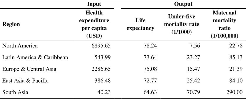
Table 1 summarizes the latest available data (from 2008) provided by the official
websites of the World Bank and the United Nations. These data, which were obtained
[image:13.612.98.516.541.710.2]from 160 different countries, were used in this analysis.
Table 1 Summary of input and output indicators by geographical and economic regions
Input Output
Region
Health expenditure
per capita (USD)
Life expectancy
Under-five mortality rate
(1/1000)
Maternal mortality
ratio (1/100,000)
North America 6895.65 78.24 7.56 22.78
Latin America & Caribbean 543.99 73.64 23.27 85.13
Europe & Central Asia 2286.65 75.08 15.47 21.39
East Asia & Pacific 386.48 72.77 25.42 84.10
Middle East & North Africa 290.72 71.98 33.62 80.10
Sub-Saharan Africa 75.27 53.24 127.91 640.00
OECD members 3983.14 78.92 9.00 24.67
European Union 3519.98 79.12 5.49 8.53
Low income 23.83 58.02 112.54 590.00
Middle income 185.28 68.54 54.33 210.00
High income 4452.57 79.36 6.74 15.18
World 863.77 69.14 60.85 260.00
A peculiarity of the health data we utilize in this paper, compared to the datasets used in
other papers dealing with the measurement of efficiency in the presence of undesirable
outputs, is that the bad outputs (under-five mortality rate, and maternal mortality ratio)
are inversely related to the good output (life expectancy) at a significance level of 0.01
(Table A2 – Appendix). For the calculation of the correlation coefficients we used Spearman’s measure as the data are not normally distributed (Table A3 – Appendix).
For the application of the generalized directional distance function model we used
direction vector (1,1,1,1), i.e., gx=(1), gy=(1), gb=(1,1). In addition, we apply the
super-efficiency DEA model under variable returns to scale (VRS) in conjunction with the
proposed generalized directional distance function method in order to identify a realistic
measurement of efficiency for the evaluated health systems. The combination of the
super-efficiency DEA under VRS and the generalized directional distance function
[image:14.612.31.587.561.709.2]models enables the ranking of the DMUs under evaluation.
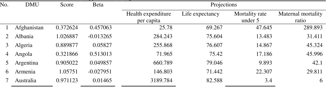
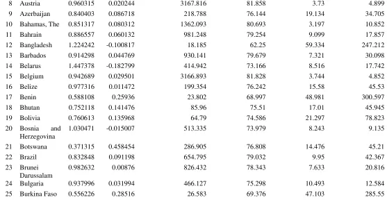
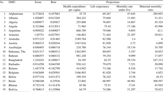
Table 2 Application of the generalized directional distance function to health data
No. DMU Score Beta Projections
Health expenditure per capita
Life expectancy Mortality rate under 5
Maternal mortality ratio
1 Afghanistan 0.372624 0.457063 25.78 69.267 47.645 289.893
2 Albania 1.026887 -0.013265 284.243 75.604 13.483 31.411
3 Algeria 0.889877 0.05827 255.868 76.607 14.867 45.324
4 Angola 0.321866 0.513013 71.965 75.42 17.186 45.996
5 Argentina 0.905022 0.049857 660.789 79.046 9.893 42.1
6 Armenia 1.05751 -0.027951 146.803 71.442 22.307 29.811
8 Austria 0.960315 0.020244 3167.816 81.858 3.73 4.899
9 Azerbaijan 0.840403 0.086718 218.788 76.144 19.134 34.705
10 Bahamas, The 0.851317 0.080312 1362.093 80.693 3.197 10.852
11 Bahrain 0.886557 0.060132 981.248 79.254 9.099 17.857
12 Bangladesh 1.224242 -0.100817 18.185 62.25 59.334 247.212
13 Barbados 0.914298 0.044769 930.141 79.679 7.321 30.098
14 Belarus 1.447378 -0.182799 414.942 73.166 8.516 17.742
15 Belgium 0.942689 0.029501 3166.893 81.828 3.744 4.852
16 Belize 0.977316 0.011472 199.354 76.242 15.58 45.53
17 Benin 0.588108 0.25936 23.802 68.997 48.981 300.597
18 Bhutan 0.752118 0.141476 85.96 75.51 17.01 45.945
19 Bolivia 0.760613 0.135968 64.79 74.586 21.297 78.823
20 Bosnia and Herzegovina
1.030471 -0.015007 513.335 73.979 8.243 9.135
21 Botswana 0.371315 0.458454 286.905 76.808 14.476 45.21
22 Brazil 0.832848 0.091198 654.795 79.032 9.95 42.367
23 Brunei Darussalam
0.982632 0.00876 826.432 78.343 7.633 20.816
24 Bulgaria 0.937996 0.031994 466.127 75.298 10.493 12.584
25 Burkina Faso 0.556226 0.28516 26.583 69.376 47.103 285.55
Table 2 displays in column 3 the super-efficiency scores of 25 out of 160 evaluated
DMUs (the full Table – Table A4 – is at the Appendices), beta (β) values in column 4, and the target values for the input, and the good and bad outputs in the following columns.
Based on the selected input and output indicators, the most efficient health system among
the 25 illustrated in Table 2 is that of Belarus (DMU 14) with a score of 1.4474, followed
by the Bangladeshi (DMU 12) and the Armenian (DMU 6) health systems which obtain
1.2242 and 1.0575 respectively. At the last places of this ranking are Angola (DMU 4)
and Botswana (DMU 21) with scores of 0.3219 and 0.3713, respectively.
The least efficient health system of the sample illustrated in Table 2, the health system of
Angola, could be regarded as (weak) efficient even if health expenditure is decreased by
51.3% compared to the original expenditure level. At the same time, in the pursuit of
efficiency attainment, life expectancy should be increased by 51.3%, and also mortality
[image:15.612.28.585.74.362.2]The data analysis displayed in Table 2, as well as in Table A4 (Appendices), proves that
the proposed method yields reasonable inefficiency measures between null and unity.
6. Conclusion
In this paper, we developed a generalized directional distance function measure for
assessing efficiency in the presence of desirable and undesirable outputs. A new
efficiency definition is introduced to overcome the inappropriateness that is associated
with the measurement of inefficiency (beta) when the direction vectors are not identical
to the inputs and outputs of the evaluated DMU. Unlike the existing directional distance
function-based measures, the proposed generalized approach is units-invariant. The
proposed method is consistent with the radial and the slack-based measures as the new
method is a generalized expression of the last two measures. In addition, the generalized
approach we put forth is flexible as it can be combined with super-efficiency DEA
models and can be extended with the incorporation of weights in its objective function.
This flexibility enhances the assessment power of the model and its applicability to real
case studies. Therefore, the proposed approach has significant managerial implications.
The properties of the new approach are presented in a numerical example utilizing health
data from 160 countries.
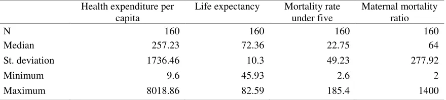
[image:16.612.88.528.581.680.2]Appendices
Table A1 Descriptive statistics of input and output indicators Health expenditure per
capita
Life expectancy Mortality rate under five
Maternal mortality ratio
N 160 160 160 160
Median 257.23 72.36 22.75 64
St. deviation 1736.46 10.3 49.23 277.92
Minimum 9.6 45.93 2.6 2
Table A2 Nonparametric correlation of input and output indicators Life
expectancy
Mortality rate under five
Maternal mortality ratio
Life expectancy Corr. Coefficient 1.000 -0.942** -0.890**
p-value . 0.000 0.000
Under five mortality rate Corr. Coefficient -0.942** 1.000 0.944**
p-value 0.000 . 0.000
Maternal mortality ratio Corr. Coefficient -0.890** 0.944** 1.000
p-value 0.000 0.000 .
**
[image:17.612.42.572.278.337.2]significant at the 0.01 level
Table A3 Testing the normality of the distributions of input and output indicators Health expenditure per
capita
Life expectancy Mortality rate under five
Maternal mortality ratio
Kolmogorov-Smirnov Test 2.042 2.596 3.495 3.558
p-value 0.000 0.000 0.000 0.000
Table A4 Application of the generalized directional distance function to health data (Part A)
No. DMU Score Beta Projections
Health expenditure per capita
Life expectancy Mortality rate under five
Maternal mortality ratio
1 Afghanistan 0.372624 0.457063 25.78 69.267 47.645 289.893
2 Albania 1.026887 -0.013265 284.243 75.604 13.483 31.411
3 Algeria 0.889877 0.05827 255.868 76.607 14.867 45.324
4 Angola 0.321866 0.513013 71.965 75.42 17.186 45.996
5 Argentina 0.905022 0.049857 660.789 79.046 9.893 42.1
6 Armenia 1.05751 -0.027951 146.803 71.442 22.307 29.811
7 Australia 0.971123 0.01465 3189.784 82.588 3.4 6
8 Austria 0.960315 0.020244 3167.816 81.858 3.73 4.899
9 Azerbaijan 0.840403 0.086718 218.788 76.144 19.134 34.705
10 Bahamas, The 0.851317 0.080312 1362.093 80.693 3.197 10.852
11 Bahrain 0.886557 0.060132 981.248 79.254 9.099 17.857
12 Bangladesh 1.224242 -0.100817 18.185 62.25 59.334 247.212
13 Barbados 0.914298 0.044769 930.141 79.679 7.321 30.098
14 Belarus 1.447378 -0.182799 414.942 73.166 8.516 17.742
15 Belgium 0.942689 0.029501 3166.893 81.828 3.744 4.852
16 Belize 0.977316 0.011472 199.354 76.242 15.58 45.53
17 Benin 0.588108 0.25936 23.802 68.997 48.981 300.597
18 Bhutan 0.752118 0.141476 85.96 75.51 17.01 45.945
[image:17.612.30.585.389.703.2]20 Bosnia and Herzegovina
1.030471 -0.015007 513.335 73.979 8.243 9.135
21 Botswana 0.371315 0.458454 286.905 76.808 14.476 45.21
22 Brazil 0.832848 0.091198 654.795 79.032 9.95 42.367
23 Brunei Darussalam
0.982632 0.00876 826.432 78.343 7.633 20.816
24 Bulgaria 0.937996 0.031994 466.127 75.298 10.493 12.584
25 Burkina Faso 0.556226 0.28516 26.583 69.376 47.103 285.55
26 Burundi 0.498206 0.33493 12.441 65.379 64.033 277.834
27 Cambodia 0.741542 0.148408 36.439 70.72 40.446 232.223
28 Cameroon 0.414126 0.414301 38.072 70.943 39.343 223.386
29 Canada 0.960704 0.020042 3189.784 82.588 3.4 6
30 Cape Verde 0.93234 0.035014 146.966 75.904 16.24 45.722
31 Central African Republic
0.421613 0.406853 11.767 64.945 65.71 267.548
32 Chad 0.397473 0.431154 27.949 69.562 46.181 278.16
33 Chile 1.006833 -0.003405 764.549 78.379 9.031 26.089
34 China 0.939244 0.03133 141.536 75.117 18.277 36.809
35 Colombia 0.8983 0.053574 300.36 76.894 14.307 45.161
36 Comoros 0.7431 0.147381 23.615 68.684 50.135 289.891
37 Congo, Dem. Rep.
0.568158 0.275382 9.655 60.654 66.797 274.032
38 Congo, Rep. 0.529908 0.307268 56.207 73.415 27.094 125.261
39 Costa Rica 1.017856 -0.008849 623.62 78.248 9.043 44.389
40 Cote d'Ivoire 0.498041 0.335077 40.424 71.263 37.754 210.658
41 Croatia 0.901974 0.051539 1166.374 79.825 5.691 13.278
42 Cuba 1.052709 -0.025678 688.745 76.53 6.462 27.391
43 Cyprus 0.945278 0.028131 1854.975 81.244 2.952 8.242
44 Czech Republic 0.938192 0.031889 1421.812 79.43 3.872 7.745
45 Denmark 0.918366 0.042554 3165.591 81.785 3.764 4.787
46 Djibouti 0.545312 0.294237 56.495 73.455 26.9 123.704
47 Dominican Republic
0.900077 0.052589 247.586 76.554 14.972 45.354
48 Ecuador 0.969168 0.015657 212.517 76.327 15.414 45.482
49 Egypt, Arab Rep.
0.918446 0.042511 93.129 75.556 16.919 45.919
50 El Salvador 0.87024 0.069382 201.875 76.259 15.548 45.521
51 Equatorial Guinea
0.311484 0.524989 258.861 76.626 14.83 45.313
52 Eritrea 1.114811 -0.054289 10.123 63.887 69.794 242.491
53 Estonia 0.878384 0.064745 1004.373 78.547 6.173 11.223
54 Ethiopia 0.765378 0.132902 11.986 65.086 65.165 270.892
55 Fiji 1.159988 -0.074069 165.123 73.174 19.548 27.926
56 Finland 0.935085 0.033546 3630.087 82.238 3.189 5.737
57 France 0.958365 0.02126 3189.784 82.588 3.4 6
58 Georgia 0.907104 0.048711 245.43 76.54 14.999 45.362
60 Ghana 0.74186 0.148198 47.23 72.191 33.158 173.837
61 Greece 3.981956 -0.598551 4971.478 78.905 4.545 3.197
62 Guatemala 0.850236 0.080943 169.092 76.047 15.961 45.641
63 Guinea 0.565927 0.277198 15.413 67.292 56.649 323.138
64 Guinea-Bissau 0.457528 0.372186 10.977 64.437 67.671 255.515
65 Guyana 0.818498 0.099808 110.096 75.666 16.705 45.857
66 Haiti 0.736249 0.151909 33.744 70.353 42.266 246.801
67 Honduras 0.908696 0.047836 114.851 75.697 16.645 45.839
68 Hungary 0.868217 0.07054 1040.177 78.901 6.528 12.083
69 Iceland 1.48 -0.193548 4022.1 81.025 3.103 5.968
70 India 0.810287 0.104797 40.528 71.174 38.052 205.897
71 Indonesia 0.884197 0.06146 47.727 72.259 32.822 171.144
72 Iran, Islamic Rep.
0.917682 0.042926 243.387 75.32 19.807 28.712
73 Iraq 0.796049 0.113555 96.51 75.578 16.877 45.906
74 Ireland 0.964651 0.017993 3128.861 80.565 4.316 2.946
75 Israel 1.000946 -0.000473 2093.662 80.964 3.28 7.003
76 Italy 0.987328 0.006376 3169.2 81.904 3.71 4.968
77 Jamaica 0.890426 0.057963 241.606 76.515 15.047 45.376
78 Japan 1.033366 -0.016409 3242.127 81.232 3.456 5.853
79 Jordan 0.897968 0.053759 307.646 76.941 14.215 45.135
80 Kazakhstan 0.747103 0.144752 284.554 76.724 17.033 38.486
81 Kenya 0.595027 0.253898 24.705 69.12 48.371 295.709
82 Korea, Rep. 0.985961 0.007069 1236.152 80.397 4.399 16.463
83 Kuwait 0.917526 0.043011 947.257 77.577 5.878 8.613
84 Kyrgyz Republic 0.944074 0.028768 52.589 71.242 39.141 78.67
85 Lao PDR 0.887995 0.059325 31.971 70.111 43.464 256.397
86 Latvia 0.838988 0.087555 893.35 78.76 9.672 18.249
87 Lebanon 0.860372 0.075054 559.026 77.455 14.99 24.049
88 Lesotho 0.32212 0.512722 29.465 69.482 46.182 258.257
89 Liberia 0.598864 0.250888 19.85 68.458 51.65 321.979
90 Lithuania 0.849351 0.08146 855.124 77.662 6.889 11.941
91 Luxembourg 0.943339 0.029156 3396.938 82.423 3.301 5.876
92 Madagascar 0.919653 0.041855 20.825 68.591 50.992 316.703
93 Malawi 0.574995 0.269846 13.07 65.784 62.47 287.421
94 Malaysia 1.073747 -0.035562 365.764 70.952 7.249 17.405
95 Maldives 0.951102 0.025062 450.484 77.711 15.402 36.073
96 Mali 0.451937 0.37747 24.111 69.039 48.773 298.926
97 Malta 0.998139 0.000931 1372.227 79.506 3.78 7.993
98 Mauritania 0.677789 0.192045 21.94 68.743 50.239 310.67
99 Mauritius 0.890055 0.05817 378.24 76.792 14.504 33.906
100 Mexico 0.939051 0.031432 569.573 78.633 10.912 44.178
101 Moldova 0.854352 0.078544 166.463 73.717 18.613 29.487
102 Mongolia 0.814621 0.102159 65.922 74.381 22.29 58.36
104 Morocco 0.880016 0.063821 139.94 75.859 16.329 45.748
105 Mozambique 0.482401 0.349162 13.362 65.972 61.745 291.87
106 Myanmar 1.265659 -0.117254 11.127 60.465 66.26 268.141
107 Namibia 0.598061 0.251517 212.816 76.329 15.41 45.481
108 Nepal 0.957322 0.021804 23.827 69 48.964 300.462
109 Netherlands 0.943421 0.029113 3189.784 82.588 3.4 6
110 New Zealand 0.953967 0.023559 2848.565 82.244 3.285 6.573
111 Nicaragua 0.933882 0.034189 101.49 75.61 16.814 45.888
112 Niger 0.580692 0.265269 15.709 67.482 55.913 327.647
113 Nigeria 0.410455 0.417982 42.742 71.579 36.189 198.117
114 Norway 0.951691 0.024753 3189.784 82.588 3.4 6
115 Oman 0.931642 0.035388 438.014 75.582 10.514 19.292
116 Pakistan 0.932477 0.034941 20.855 66.983 56.72 250.915
117 Panama 0.938271 0.031847 477.465 78.038 12.074 44.514
118 Papua New Guinea
0.770666 0.129519 33.955 69.693 44.58 217.62
119 Paraguay 0.892626 0.056733 152.323 75.939 16.173 45.702
120 Peru 0.924112 0.039441 192.331 76.197 15.669 45.556
121 Philippines 0.837425 0.08848 62.007 74.005 23.896 85.683
122 Poland 1.249808 -0.111035 1079.158 75.038 7.089 6.666
123 Portugal 0.930742 0.035871 2346.55 81.341 3.953 6.749
124 Qatar 0.929876 0.036336 1710.46 80.601 3.152 7.709
125 Romania 0.882694 0.062308 484.582 77.087 15.003 25.318
126 Russian Federation
0.756497 0.13863 489.347 77.255 11.542 33.593
127 Rwanda 0.545962 0.293693 32.084 70.126 43.388 255.786
128 Saudi Arabia 0.888261 0.059175 635.996 77.746 13.836 22.58
129 Senegal 0.615533 0.237982 47.191 72.186 33.184 174.047
130 Serbia 1.205675 -0.093248 545.165 75.143 8.431 8.746
131 Sierra Leone 0.345076 0.486905 24.044 69.03 48.818 299.287
132 Singapore 2.299574 -0.393861 1956.497 78.229 3.903 12.545
133 Slovak Republic 0.941865 0.029938 1353.425 76.941 5.766 5.82
134 Slovenia 0.931713 0.035351 2158.96 81.55 3.054 7.731
135 Solomon Islands 0.812305 0.103567 60.556 73.579 25.19 89.643
136 South Africa 0.340331 0.492169 232.934 76.459 15.157 45.408
137 Spain 0.971971 0.014214 3087.836 82.329 3.587 5.915
138 Sri Lanka 1.125073 -0.058856 87.459 73.807 18.636 41.295
139 Suriname 0.803269 0.109097 376.811 77.388 13.343 44.882
140 Swaziland 0.277404 0.565675 61.391 74.122 23.593 97.213
141 Sweden 0.9881 0.005985 3981.455 81.585 3.181 4.97
142 Switzerland 0.985594 0.007255 3189.784 82.588 3.4 6
143 Syrian Arab Republic
1.281653 -0.123443 79.603 74.106 19.323 51.678
144 Tajikistan 1.341162 -0.145724 42.839 66.786 57.025 73.326
145 Tanzania 0.637781 0.221164 17.25 68.104 53.407 336.047
147 Timor-Leste 0.662131 0.203275 56.852 73.503 26.659 121.773 148 Trinidad and
Tobago
0.747529 0.144473 776.443 79.318 8.789 36.947
149 Tunisia 0.942311 0.029701 240.711 76.509 15.059 45.379
150 Turkey 0.89163 0.057289 587.569 77.319 13.747 21.682
151 Turkmenistan 0.722759 0.160929 68.445 75.084 18.828 59.045
152 Uganda 0.50374 0.330017 29.296 69.746 45.27 270.87
153 Ukraine 0.874697 0.066839 250.063 72.813 13.064 24.262
154 United Arab Emirates
0.893919 0.056011 1347.031 80.491 3.363 9.44
155 United Kingdom 0.927651 0.037532 3189.784 82.588 3.4 6
156 United States 0.887428 0.059643 3189.784 82.588 3.4 6
157 Uruguay 0.939041 0.031438 701.785 78.369 11.623 26.151
158 Uzbekistan 2.6333 -0.449536 74.486 73.038 26.518 43.486
159 Yemen, Rep. 0.745385 0.145879 56.8 73.496 26.694 122.052
160 Zambia 0.337952 0.494822 34.534 70.335 42.179 237.434
References
[1] Charnes A, Cooper WW, Rhodes E. Measuring the efficiency of decision making units. Eur J Oper Res. 1978;2(6):429-44.
[2] Chung YH, Färe R, Grosskopf S. Productivity and undesirable outputs: A directional distance function approach. J Environ Manage. 1997;51(3):229-40.
[3] Fare R, Grosskopf S, Lovell CAK, Pasurka C. Multilateral Productivity Comparisons When Some Outputs Are Undesirable - a Nonparametric Approach. Rev Econ Stat. 1989;71(1):90-8.
[4] Scheel H. Undesirable outputs in efficiency valuations. Eur J Oper Res. 2001;132(2):400-10.
[5] Seiford LM, Zhu J. Modeling undesirable factors in efficiency evaluation. Eur J Oper Res. 2002;142(1):16-20.
[6] Tone K. Dealing with Undesirable Outputs in DEA:A Slacks-based Measure (SBM) Approach. The Operations research Society of Japan2004. p. 44-5.
[7] Yang H, Pollitt M. Incorporating both undesirable outputs and uncontrollable variables into DEA: The performance of Chinese coal-fired power plants. Eur J Oper Res. 2009;197:1095–105.
[8] Yu M-M, Hsu S-H, Chang C-C, Lee D-H. Productivity growth of Taiwan's major domesthic airports in the presence of aircraft noise. Transportation Research Part E. 2008;44:543–54.
[9] Lozano S, Gutierrez E. Slacks-based measure of efficiency of airports with airplanes delays as undesirable outputs. Computers & Operations Research. 2011;38(1):131-9. [10] Podinovski VV, Kuosmanen T. Modelling weak disposability in data envelopment analysis under relaxed convexity assumptions. 2011;211:577–85.
simultaneous input–output projection in data envelopment analysis. Computers and Operations Research. 2011;38(2):496-504.
[12] Tone K. A slacks-based measure of efficiency in data envelopment analysis. Eur J Oper Res. 2001;130(3):498-509.
[13] Cheng G, Qian Z. Data Normalization for Data Envelopment Analysis and Its Application in Directional Distance Function. Systems Engineering. 2011;29(7):70-5. [14] Zaim O, Fare R, Grosskopf S. An economic approach to achievement and improvement indexes. Soc Indic Res. 2001;56(1):91-118.
[15] Retzlaff-Roberts D, Chang CF, Rubin RM. Technical efficiency in the use of health care resources: a comparison of OECD countries. Health Policy. 2004;69(1):55-72. [16] Afonso A, St Aubyn M. Non-parametric approaches to education and health efficiency in OECD countries. J Appl Econ. 2005;8(2):227-46.
[17] Grosskopf S, Self S, Zaim O. Estimating the efficiency of the system of healthcare financing in achieving better health. Applied Economics. 2006;38(13):1477-88.
[18] Lantz PM, Ubel PA. The Use of Life Expectancy in Cancer Screening Guidelines. Journal of General Internal Medicine. 2005;20(6):552-3.
[19] Wilson J, Graham J, MacDonagh R. Patient life-expectancy: a vital element in planning treatment? BJU International. 2004;93(4):461-3.
[20] Weinstein M, Appadoo S. CREATIVE APPROACHES TO MODELING LIFE EXPECTANCY GAINS FOR ECONOMIC EVALUATION USING PUBLISHED DATA. Value Health. 2001;4(2):189-90.
[21] Rajaratnam JK, Tran LN, Lopez AD, Murray CJL. Measuring Under-Five Mortality: Validation of New Low-Cost Methods. PLoS Med. 2010;7(4):e1000253.
[22] Hegyvary ST, Devon MB, Murua A. Clustering Countries to Evaluate Health Outcomes Globally. Journal of Public Health Policy. 2008;29(3):319-39.
[23] Rutherford ME, Mulholland K, Hill PC. How access to health care relates to under-five mortality in sub-Saharan Africa: systematic review. Tropical Medicine & International Health. 2010;15(5):508-19.
[24] Loudon I. The Transformation Of Maternal Mortality. BMJ: British Medical Journal. 1992;305(6868):1557-60.
[25] Shiffman J. Can Poor Countries Surmount High Maternal Mortality? Studies in Family Planning. 2000;31(4):274-89.
[26] Kao S, Chen L-M, Shi L, Weinrich MC, Miller CA. Maternal Mortality in Taiwan: Rates and Trends. International Family Planning Perspectives. 1997;23(1):34-8.
[27] Mauldin WP. Maternal Mortality in Developing Countries: A Comparison of Rates from Two International Compendia. Population and Development Review. 1994;20(2):413-21.
[28] Bhatia JC. Levels and Causes of Maternal Mortality in Southern India. Studies in Family Planning. 1993;24(5):310-8.