An appraisal of the wealth effect in the US: evidence from pseudo panel data

Munich Personal RePEc Archive

An appraisal of the wealth effect in the

US: evidence from pseudo-panel data

Salotti, Simone

Department of Economics, National University of Ireland, Galway

April 2010

Online at

https://mpra.ub.uni-muenchen.de/27351/

An appraisal of the wealth effect in the US: evidence from

pseudo-panel data

This draft: December 2010

Simone Salotti

Department of Economics, National University of Ireland Galway

Abstract. How does household wealth influence consumption? The empirical evidence brought so far by the literature is unclear, mostly because of the low quality of the data

more readily available: aggregate data, cross sections and panel datasets lacking important

variables all present major shortcomings for a proper analysis of the wealth effect. The aim

of our paper is to contribute to the appraisal of the wealth effect performing a pseudo-panel

analysis for the USA (1989-2007), combining information from the Consumer Expenditure

Survey and the Survey of Consumer Finances. We distinguish between total and non

durables consumption, and we also investigate the roles of the different components of

household wealth, both gross and net. Our estimates indicate that there is a significant

tangible wealth effect (between 2 and 4 cents per dollar), with an overwhelming importance

of the value of the house of residence. On the contrary, financial wealth seems to positively

affect consumption of the older households only. In general, it seems that older households

experience higher wealth effects, i.e., extract more liquidity from their assets, than younger

ones, which rely more on income effects.

Keywords: consumption; household wealth; wealth effect; pseudo-panel.

JEL: D12, E21



1. Introduction

Aggregate savings rates in the USA have declined considerably during the Nineties and the

beginning of the new Millennium (Hüfner and Koske 2010). Due to the contemporary growth of

stock prices up to 2000, and of housing prices afterwards, many economists (Bernanke 2005;

Paiella 2007a) have seen a direct relationship between the two phenomena thanks to the so called

‗wealth effect‘ channel. F.i. Greenspan (2003) credited housing wealth, realized capital gains, and home equity borrowing with shoring up the economy in the aftermath of the stock market collapse

of 2000 and the 2001 recession, primarily through their effects on consumer spending. Accordingly,

Juster et al. (2005) claim that the decline in the personal saving rate is due to the significant capital

gains in corporate equities experienced over this period. On the other hand, others conclude that

there is at best a weak evidence of a stock market wealth effect, and underline the importance of

housing wealth in determining the households‘ decisions on consumption and savings (Case et al. 2005).

However, the mechanism through which wealth affects consumption is not yet clearly understood:

while the arguments supporting a direct wealth effect are clear (changes in wealth directly cause

changes in consumption through their effect on households' contemporaneous budget sets), the

empirical evidence brought so far by a large literature that investigates the role of wealth shocks on

consumption is unclear. Moreover, wealth can affect consumption through the indirect channel of

providing collateral for obtaining access to credit (Cynamon and Fazzari 2008). In light of that, the

aim of our article is to explore deeply the influence of wealth on household consumption and

savings.

In our article we overcome the well known problem of inappropriate and incomplete data (which is

partly responsible for the mixed results produced by the previous empirical literature) using a

pseudo-panel dataset that combines information from two different surveys, the Consumer

Expenditure Survey (CES) and the Survey of Consumer Finances (SCF). First, we impute the SCF

wealth variables to the CES households for which we have detailed consumption data (that is, we

use the SCF as a donor to enrich the variables set of the CES).1 Then, we construct panel data from

the resulting time series of cross sections employing a methodology introduced in Browning et al.

(1985) and Deaton (1985). These pseudo-panel data can be used as a substitute for the unavailable

true panel data to answer long-term individual behavioural questions such as the one addressed in

this paper. After having defined cohorts based on time-invariant parameters (i.e. year of birth), the

mean values for each variable of interest become the observations in the pseudo-panel data. In

addition to filling gaps in the availability of true panel data, Deaton (1985) identifies three

single set of pseudo-panel data if comparable cohorts can be defined in each source. Attrition

problems often found in true panel data are minimized. The problem of the individuals‘ response

errors is smoothed by the use of cohort means and can be explicitly controlled by using

errors-in-variables method.

Our analysis exploits all these features using the pseudo-panel dataset to estimate a consumption

equation with wealth, in various decompositions, as one of the main explanatory variables, for the

period 1989-2007. In our analysis we differentiate between financial and tangible wealth, the latter

further disaggregated into the value of the house of residence and the other tangible assets (mainly,

other real estate properties). In addition, we investigate the role of debt on consumption decisions

by studying both gross and net wealth. We also devote particular attention to the consumption

behaviour of the older households, since both theory and previous empirical evidence suggest that

they behave differently from younger households (f.i. see Miniaci et al. 2010).

The main result of our study is that tangible wealth is the main type of household wealth to

positively affect consumption. In particular, the house of residence is the component of tangible

wealth responsible for the highest direct wealth effect. The estimated elasticity of consumption

spending with respect to the value of the house of residence is between two and four cents per

dollar, which is not far from previous estimates. We view these estimates as a lower bound for the

actual effects, since we study the effects of three year changes in wealth on one year consumption

only (due to the triennial nature of the SCF). Among the additional results, older households

experience a higher wealth effect (i.e. they extract more liquidity from their assets, as predicted by

theory). This is particularly evident for net financial wealth, while it is measured with lower

precision for the rest of the household wealth.

It would be tempting to use our results to comment on the economic and financial crisis that

originated from the subprime mortgage market in 2007. However, we believe it to be impossible to

extend our results to the interpretation of the consumption and saving dynamics from the beginning

of the crisis onwards, not only because we employ data up to 2007 only, but also because it would

be implausible to assume that wealth effects of the same magnitude are at work both during booms

and during recessions. Indeed, some studies investigated the asymmetry of consumption responses

to increases and decreases in wealth (f.i. Shirvani and Wilbratte 2000; Bertaut 2002; Disney et al.

2003). The rationale behind the unequal wealth effects relates to the assumption of diminishing

marginal utility of wealth, where preferences are represented by convex utility functions (reflecting

risk aversion) such that consumers would value increases in wealth less highly than equivalent

reduction, some consumers may find it difficult to borrow to increase consumption. Thus, our

analysis is unable to shed light on the mechanisms at work during the recent financial crisis.

The rest of this paper is organized as follows. Section 2 provides a brief review of the previous

literature. Section 3 describes the data used and how they were combined. Also, the econometric

models are presented. Section 4 illustrates the results. Section 5 concludes briefly.

2. The wealth effect in the literature

There is a large literature devoted to the study of the wealth effect. Most of it is based on the

life-cycle model originally proposed by Ando and Modigliani (1963). According to this theory, an

increase in wealth leads the individuals to gradually increase consumption. Also, the propensity to

consume out of wealth, whatever its form, should be the same small number (Paiella 2007b). In

practice, this is likely to be violated, ―if assets are not fungible and households develop ‘mental accounts‘ that dictate that certain assets are more appropriate to use for current expenditure and

others for long-term saving‖ (Paiella 2007b, 191). Thus, the appraisal of the wealth effect is an

empirical matter, and a fair number of articles have dealt with it. Consequently, a wide range of

estimates have been produced. For the US economy, they usually lie between 2 and 7 cents of

additional consumption per year per 1 dollar increase in household wealth. This is consistent with

the magnitude of the effect estimated by the research staff of the Board of Governors of the Federal

Reserve System, that maintains the longest and most regularly updated wealth effect estimates for

the USA. However, there are significant differences in the results depending on the methods

utilized.

Aggregate data analysis typically find positive effects of wealth increases on private consumption

(Davis and Palumbo 2001; Mehra 2001). Also, the real estate wealth effect seems to be higher than

the stock market wealth effect. This arises from studies that concentrate either on the former

(Girouard and Blondal 2001; Belski and Prakken 2004; Catte et al. 2004), the latter (Ludvigson and

Steindel 1999; Poterba 2000; Edison and Sløk 2002; Sousa 2003; Liu and Shu 2004; Case and

Quigley 2008), or both (Ludwig & Sløk 2002; Benjamin et al. 2004; Case et al. 2005). As it is

common in the empirical literature, some authors find opposite results on the relative importance of

the two types of wealth effects (f.i. Dvornak and Kohler 2007). There is no widespread agreement

on the econometric techniques to adopt, either. In particular, some studies try to disentangle the

short run effects of wealth changes from the long run ones, due to the concern that wealth shocks

must be perceived as permanent in order to affect consumption. While most of them adopt

2003; Lettau and Ludvigson 2004), some authors choose alternative ways (f.i. Carroll et al. 2006;

Morris 2006).

However, the use of aggregate data has been criticized because of its inability to solve the

well-known problem of endogeneity, which is present due to the fact that wealth is the result of both past

savings/consumption decisions and movements of asset prices. Attanasio and Banks (2001) advise

not to use aggregate data also because of aggregation issues and difficulties in decomposing age,

cohort and time effects. Also, household-level data may permit to distinguish between durables and

non-durables consumption (f.i., see Fernandez-Villaverde and Krueger 2007), and, on the wealth

side, among different components of both tangible and intangible wealth (f.i. see Juster et al. 2005).

Accordingly, a whole strand of literature uses household-level data to investigate the magnitude of

the wealth effect. While there are few studies on economies outside the US (Campbell and Cocco

2007 on the UK; Paiella 2007b on Italy), most of them concentrate on the US economy (Engelhardt

1996; Skinner 1996; Parker 1999; Dynan and Maki 2001; Lehnert 2004; Juster et al. 2005). This is

due to the availability of many US survey and panel data, such as the Consumer Expenditure

Survey (CES), the Panel Study of Income Dynamics (PSID), or the Survey of Consumer Finances

(SCF). However, each one of them, taken singularly, has some drawbacks for this type of analysis.

The PSID contains data on food consumption only, and data on household wealth have been

collected since 1984 every five year only. The CES has highly detailed consumption data, but the

quality of its wealth data is low due to limitations both in scope and precision. On the other hand,

the SCF does not contain detailed consumption variables, while information on wealth is collected

very accurately. Some authors (f.i Maki and Palumbo 2001) tried to overcome these problems by

using cohort-level analysis based on the original ideas by Browning et al. (1985) and Deaton (1985)

by combining aggregate and household level data. An interesting alternative is the one by Bostic et

al. (2009), where a sample combination technique has been used to obtain a dataset suitable for an

analysis of the wealth effect.

Generally, household-level data studies tend to confirm the results of the studies that use aggregate

data (Levin 1998, is a notable conflicting example, since he concludes that wealth does not affect

consumption), but have a higher ability to distinguish between different channels through which

wealth changes affect consumption. Also, depending on the data used, some of them have been able

to shed light on the role of liquidity constraints and precautionary savings (f.i. Engelhardt 1996, and

Campbell and Cocco 2007, respectively).

The strategy followed in our paper is to build a new pseudo-panel dataset combining information

from existing US sources. A sample combination procedure is used to enrich the CES data with

pseudo-panel analysis. The procedure generates a dataset which contains a large amount of

information, which helps dealing with the problem of omitted variables, and therefore moderates

the issue of endogeneity. Methods of integrating different sources of information similar to the one

that we utilized here have been recently used by some national institutes of statistics as a convenient

way to obtain detailed datasets without having to bear the costs of producing brand new surveys

(f.i., see Rosati 1998; Del Boca et al. 2005). We follow closely the guidelines established in the

literature (D‘Orazio et al. 2006; Ridder and Moffitt 2007), then we use the resulting dataset to build a pseudo-panel, following the idea originally proposed by Browning et al. (1985) and Deaton

(1985). Finally, we provide data and codes that we used to perform whole analysis in order to

ensure its repeatability (see the Web Appendix).

3. Data: sample combination and pseudo-panel characteristics

3.1 CES and SCF data

In our analysis we use the wealth data from the SCF to enrich the information contained on the

CES, that contains detailed consumption data, for the period 1989-2007.2 The dataset arising from

the combination of these two surveys contains data on both consumption and wealth, making it the

appropriate source for the analysis of wealth effect. Also, there is a rich set of additional

socio-economic variables that helps attenuating the problem of endogeneity related to omitted variables.

The CES is collected by the Bureau of Labor Statistics (BLS) to compute the Consumer Price

Index, and contains data on a high percentage of total household expenditures (see Garner et al.,

2006). It is a rotating panel in which each household is interviewed four consecutive times over a

one year period. Each quarter 25% of the sample is replaced by new households. The survey

contains quarterly data, thus we had to extrapolate data on yearly consumption to perform the

combination with the SCF. Also, the interviews are conducted monthly about the expenditures of

the previous three months: for example, a unit interviewed in January will appear in the same

quarter of a unit interviewed in February or March, even if the reported information will cover a

slightly different period of time. This overlapping structure of the sample complicates the operation

of estimating annual consumption in many dimensions. First, the year over which we have

information for each household is different depending on the month in which the household

completes its cycle of interviews. Second, and even more important, not all households complete

the cycle of four interviews, thus they don't report all the expenditures made in one year. What

follows is a detailed explanation of the procedure that we followed to obtain annual data from the

In order not to waste a vast amount of information, we have chosen to use the data of the

households present for the whole year of reference, as well as the data of the households that were

interviewed three periods or less. First, we harmonized the expenditure variables using the

Consumer Price Index (CPI), differentiated for food, energy and other goods, in order to have all

expenditures expressed with the prices of June of the reference year. Second, we seasonally

adjusted the quarterly measures of consumption using the ratio to moving average method. Finally,

we used a simple technique to extend these corrected quarterly expenditures to the whole year of

interest: we multiplied by four the expenditure of the households present for one quarter only, by

two the expenditure of two quarters and by four thirds the expenditure of the households

interviewed for three quarters. For the households that were present for four quarters in a row, we

just computed the sum across quarters. We believe that this procedure does not produce distorted

measures according to the number of quarters for which there are data in the CES, due both to the

CPI harmonization and, even more important, the seasonal adjustment. We also checked whether

this operation led to a dataset differing from the original (quarterly) one in terms of distributions of

the variables that we used in our analysis, finding no significant differences. For each household, in

addition to the consumption variables, both for total and non-durables expenditure, we kept

socio-demographic variables and annual income.3

The household wealth data that we imputed to the CES households come from the SCF, which is

triennial and is produced by the Federal Reserve Board. This survey contains socio-demographic

information that proved valuable for the statistical matching procedure. In particular, we used data

on marital status, race, age, education and occupation of the household head, home ownership status

and family size. The period covered by the analysis starts in 1989, mainly because the SCF question

frame was different in earlier periods, and ends in 2007, with 7 periods in total. In addition, we used

the information contained in all the five implications of the SCF (five different versions of the

dataset that derive from the multiple imputation procedure used to approximate the distribution of

missing data, as explained by Kennickell 1998), by performing the sample combination with the

CES separately for each implication.

3.2 The sample combination procedure

The aim of the procedure is to look for similar households across the two surveys and then to attach

the wealth variables observed for the SCF households to the most similar ones in the CES, so to get

an ―augmented‖ CES that contains detailed information on wealth in addition to the consumption

and socio-demographic variables originally collected by the BLS. In constructing and applying the

so to make sure to produce a high quality new dataset. The details of the procedure are the

following.4

We first partitioned both samples into cells based on six categorical variables in order to avoid

matching individuals that differ in important characteristics. For the year 2007, and similarly for the

other years, more than 700 cells were created using:

* Race - white, black or other;

* Marital status - married or not;

* Education - twelfth grade or less, high school, some college or more;

* Tenure - home owner or not;

* Occupation - not working, managers and professionals, technicians, services, operators, other;

* Family size - one, two, three or four or more people in the household.

Thanks to this detailed partition that makes use of many different variables, we were able to avoid

the risk of matching pairs of households differing in fundamental characteristics. Almost every cell

contained individuals from both surveys, and the imputation of the wealth variables to the CES

households has been done only using SCF households pertaining to the same cell. Thus, within

every cell, we looked for the most similar households across the two surveys according to the

values of income and age, building a unique distance function able to measure the differences in

these two variables.5 The wealth values of the SCF households were assigned to the most similar

CES households within the cell. We also refined the matching by dropping the individuals for

which the distance function displayed too high value, that is, the matched individuals had

non-deniable differences in age and/or income to be paired together.6 The matching process yielded a

dataset with more than 12,000 observations in 2007.

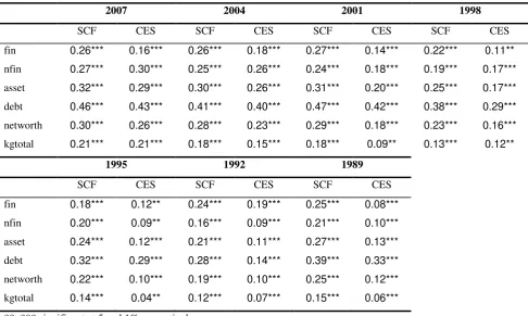
We checked the result of the matching procedure in two different ways. We verified the similarity

among the correlations between income (which is observed in both surveys) and the wealth

variables both in the SCF and in our augmented CES (after-matching). Table 1 shows that the

similarity is very high, suggesting that the procedure did not alter the distribution of the imputed

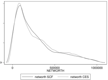
variables, a signal of good quality of the overall sample combination. Furthermore, we produced the

graphs of the probability density functions of the matched variables obtained with a kernel density

estimation, finding comfortingly similar curves.

insert Table 1 about here

insert Figures 1-7 about here

Figures 1-7 report the graphs for household net wealth: we have chosen this variable because it

comprehends both assets and debt, therefore it summarizes more than other variables the results of

the SCF individuals are used as donors in the matching procedure, the curves do show very similar

patterns, again making sure that the matching procedure maintained the distributional properties of

the variables of interest.

We used these precautions because sample combination methods must be applied with care, as there

are some conditions that have to be met in order not to commit errors. First, the two different

surveys must be two samples drawn from the same population. Second, there must be a set of

common variables on which to condition the matching procedure, as it is clear from the above

description of the procedure. As for the first condition, both the CES and the SCF are samples

representing the US population. Their sample designs are different, since the SCF oversamples

households that are likely to be wealthier, while the CES does not. However, we decided to proceed

with the sample combination procedure without correcting for this difference, since any correction

(that is, dropping a certain percentage of the wealthier SCF households) would have involved a high

degree of subjectivity. Despite this fact, the resulting dataset is robust to the alternative modus

operandi where the wealthiest SCF households are dropped before the sample combination.7 About

the second condition, there are many socio-demographic variables that are collected in both

surveys, and for some of them a recoding proved to be necessary to express them in the same way.

This has been carried out making a large use of the documentation that accompanies the public

releases of the two surveys. Most recoding operations turned out to be straightforward. The most

interesting exception has been the recoding of the occupational sector variable for the 1989 and

1992 waves of the CES, where there is an additional category, "self-employed", that in the SCF is

not taken into account. In this case we performed a multinomial logit estimation to impute the

occupational sector to the CES individuals labeled as "self-employed" in order to proceed with the

matching with the SCF. The estimation results were in line with the distributions of the

occupational variable both in the SCF and in the subsequent editions of the CES.

3.3 Pseudo-panel: construction and characteristics

Following Browning et al. (1985) and Deaton (1985), we constructed panel data from the time

series of cross sections resulting from the sample combination procedure. This method allows us to

overcome the major limitation of repeated cross-sectional data, i.e. the fact that the same individuals

are not followed over time. Pseudo-panel data present the additional advantage of dealing with the

attrition problem more flexibly with respect to genuine panel data.

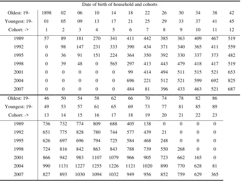
In this section we define cohorts based on the year of birth of the household head. Each cohort

consists of households whose head was born within four-year period: the oldest cohort is for

1989. The resulting dataset is composed by 23 cohorts and 7 years of data (see Table 2 for more

details).

Insert Table 2 about here

Figure 8 plots the evolution of the ratio of net wealth over income over the life cycle. Each line

corresponds to a different cohort. It is interesting to notice that the ratio rises somewhat constantly

starting from the beginning of the age of majority, until it experiences a decline between 70 and 80

years old.8

Insert Figures 8-9 about here

Figure 9 is built in a similar way, and shows the ratio of non durables consumption on income over

the life cycle. The profiles are hump-shaped over the life cycle, reflecting the evolution of the

income profiles. At the beginning of the age of majority income is typically low, leading to values

of the ratio larger than one. Then, as income rises, this kind of expenditure represents a declining

share of it (reaching a minimum of approximately .5), until the age of retirement, when income

decreases due to retirement.

4. Model and results

4.1 The model

Following the literature on life cycle consumption, the basic specification of our model would be

the following, if household-level panel data were available:

'

1 2

log(Cit) log(incomeit) log(wealthit)Zit ki it (1)

where Cit is consumption (either total or non durables consumption); incomeit is current income;

wealthit is household wealth; ki is a fixed (time-invariant) individual effect; Zit is a vector of

additional controls; it is a time-varying and individual-specific error term.

However, we estimate a similar model based on a pseudo-panel, thus equation (1) has to be

aggregated over all individuals within a specific cohort. We obtain the following model that refers

to cohorts rather than individuals (indexed by c, instead of i):

__ _________ __ __ __

'

1 2

log(Cct) log(incomect) log(wealthct) Zctkctct (2)

where the variables are the cohort means. Note that, differently from the individual fixed effect in

equation (1), the mean of the cohort effect is no longer necessarily constant over time, since the

pseudo-panel is composed by independent cross sections, so that the same individuals are not

present in more than one of them. It can be expected that the cohort effect will be correlated with

the explanatory variables, leading to inconsistent estimates. Deaton (1985) solves this problem by

error-ridden measurements of these means, thus suggesting an error-in-variables estimator. We

therefore estimate a fixed effects model, correcting for the measurement errors in observed cohort

means.

In our analysis we use three different specifications of the model in equation (2), in order to

investigate the role of the different components of household wealth. Specification 1 divides wealth

between the value of the house of residence (house), the value of the rest of tangible assets (mostly

other real estate properties, ore) and gross financial wealth (fin); the other two specifications

investigate the role of household debt. Specification 2 includes financial wealth net of debt (netfin),

while specification 3 includes gross financial wealth together with the total value of tangible assets

diminished by debt (nettng). The additional explanatory variables of the model are the following:

annual income (income), age (age and agesq), educational level (educ), two dummies for the race

(race-black for African Americans, race-other for other non-White), a dummy for the occupational

status (not working). We also include a few interaction variables in order to better grasp the wealth

and consumption dynamics of the old people. In particular, a dummy that takes the value of 1 if the

household head is over 65 years old is multiplied by income and by the relevant (according to the

various model specifications, see below) income and wealth variables.

Notice that in principle, when trying to explain the observed variance of the variables, we would

like to be able to differentiate between cohort effects, age effects and period effects. However, as

noted by Russell and Fraas (2005), these three effects ―cannot be simultaneously identified because

only one time dimension and one individual or cohort dimension exists. More specifically, the

functional relationship between all three effects causes perfect collinearity when all three effects are

fully specificied (Fienberg & Mason, 1985; Ryder, 1965)‖ (Russell and Fraas 2005, 3). We address

the age, period and cohort identification problem by using a linear restriction that all period effects

are equal, therefore we do not include year dummies among the controls. This assumption allows a

set of mean age dummies, and the fixed effects estimation takes into account the cohort effects.

We estimate these three specifications using two alternative dependent variables: the logarithms of

total consumption and of non-durable goods expenditure. We disregard the expenditure on durable

goods because its timing does not match the flow of services coming from the goods. In particular,

the relationship between consumption, income and wealth applies to the flow of consumption, but

durable goods expenditure ―represents replacements and additions to a stock, rather than the service

flow from the existing stock‖ (Paiella 2007b, 198). This is why we concentrate on the results for

total and, above all, non durable goods consumption.9

All the fixed effects estimations take into account the multiple imputation used in the SCF using the

RII (see Montalto and Sung 1996; Rubin 1987). Very briefly, every year the SCF consists of five

complete data sets because missing data are multiply imputed, producing implications 1 to 5. For

each survey year, we performed the sample matching with the CES separately for every implication,

thus obtaining five different datasets for each year of interest (1989, 1992... and 2007). Then, in

order to get the whole time series of cross-sections, we aggregated all the implications 1, then all

the implications 2, and so on until the implications number 5, obtaining 5 different implications of

the same dataset, from which obtaining our pseudo-panel.10 Thanks to the RII, we use information

from all these five data sets in order to make valid inferences, taking into account the extra

variability in the data due to the imputed missing values. Also, standard errors are clustered, as it is

advisable using pseudo-panel data (Petersen 2009).

Insert Tables 3-5 about here

The results of the estimation of equation (2) (131 non empty cohorts, obtained from more than

73,000 observations for each implication) are reported in Tables 3-5, because of the three

specifications based on the different decompositions of household wealth. In each table, results are

reported separately for models with the two different dependent variables. Results show that current

income positively and significantly affected consumption in the period 1989-2007. The estimated

elasticity ranges between 0.47 and 0.62, indicating that current income plays a very important role

in determining current consumption. Turning to the household wealth coefficients, it seems that its

various components differently affect consumption. In particular, gross financial wealth did not

positively affect consumption during the period of interest (the fin coefficients are always very

small and negative). On the contrary, tangible wealth positively affected consumption, with an

estimated elasticity reaching at most 4 cents per dollar (see the house coefficient in Table 3 when

non durables expenditure is the dependent variable). In particular, the estimated coefficients

associated to the house of residence are always highly significant, while the ones of the other

tangible assets, although always positive, are not statistically different from zero at standard

significance levels.

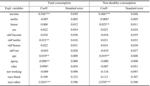
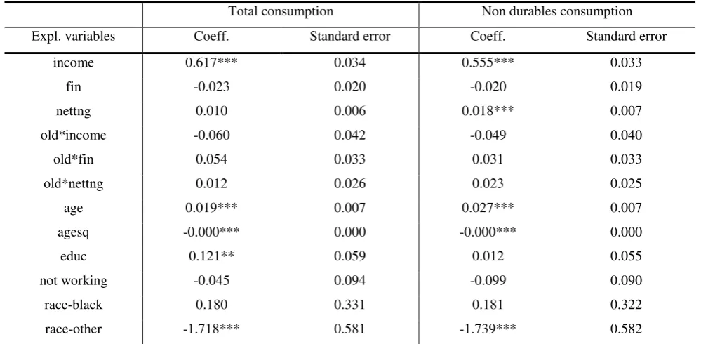
Once debt is introduced in the analysis, with the estimation of the second and third specifications,

results show that considering tangible wealth net of debt lowers the estimated elasticity (1 and 2

cents per dollar with total consumption and non durables expenditure as dependent variables,

respectively - see Table 4), but remains significantly different from zero when the dependent

variable is non durables expenditure.

The behaviour of the older households is investigated thanks to the income and wealth interaction

housing wealth are always positive, suggesting that older households extract more liquidity out of

their properties. However, these estimates suffer from a low precision, as only the coefficient of the

interacted net financial wealth (Table 4, total consumption as the dependent variable) is statistically

significant at standard levels (showing an elasticity of 2 cents per dollar). Finally, the old*income

interaction term shows that older households rely less on income when deciding their consumption

levels, since the estimated coefficients are always negative.

The rest of the explanatory variables present the following results. The non trivial relationship

between age and consumption is confirmed by the high statistical significance of the coefficients of

age and age squared (the first positive, the second smaller and negative). Higher education is

associated with higher consumption, while of the two ethnic-minorities dummies, only the one

indicating a non-White and non-Black household head is always negative and statistically

significant (the reference ethnic group is White).

We investigated the robustness of our findings in several ways. The results hold when we get rid of

the 1% of household that are at the top and at the bottom both of the income and of the consumption

distributions. As said previously, the results are also robust to variations of the sample combining

procedure. This robustness is not surprising, since our sample is very large, and it is unlikely that

our results are driven by outliers or by small subsamples of households.

To conclude, wealth surely plays a role in determining consumption and savings patterns of

American households during the period 1989-2007. However, the phenomenon is multi-faceted,

since various kinds of wealth affect consumption in different ways. In particular, financial wealth

does not seem to exert positive effects on it, while tangible wealth does, particularly through the

value of the house of residence. Additionally, the direct wealth effect phenomenon is more

important for older households, while the younger ones rely more on current income when deciding

their expenditure levels.

5. Conclusions

This paper analyses the strength of the wealth effect on consumption in the USA with a

pseudo-panel dataset specifically built for this scope. We combine data from the CES and the SCF for the

years 1989-2007. In particular, the SCF was used as the ―donor‖ survey: its wealth data were given

to CES households in order to enrich the data collected in this latter survey and to perform an

analysis capable to link consumption and wealth using household-level data. This sample

combination produced a large time series of cross sections with more than 70,000 observations. The

resulting dataset was then used to build a pseudo-panel dataset aggregating individual observations

households whose head was born within four-year period: the oldest cohort is for individuals born

between 1898 and 1901, and the youngest for individuals born between 1986 and 1989. The

resulting dataset is composed by 23 cohorts and 7 years of data. The effects of wealth were

investigated using two different dependent variables: total and non durables consumption. Our

dataset permits a high disaggregation of tangible wealth, as well as a differentiation between net and

gross financial wealth. We differentiate between financial and tangible wealth, the latter further

disaggregated into the value of the house of residence and the other real estate properties; in

addition, we investigate the role of debt on consumption decisions by studying both gross and net

wealth.

The main result of our study is that tangible wealth is the main type of household wealth to

significantly and positively affect consumption during the period 1989-2007. The estimated

elasticity of consumption spending with respect to tangible wealth is between 2 and 4 cents per

dollar, which is not far from previous estimates. In particular, the house of residence is the part of

tangible wealth which is responsible for the highest direct wealth effect. It seems that households

tend to consume both out of their house of residence and out of their other real estate properties,

even if the latter effect is estimated with lower precision. On the other hand, our results suggest that

financial wealth exerts a positive direct effect on household consumption for the older households

only. Among the additional results, older households experience a higher tangible wealth effect

(that is, extract more liquidity from their assets, as predicted by theory), while they have a lower

elasticity of consumption with respect to income.

It would be tempting to use our results to comment on the economic and financial crisis that

originated from the subprime mortgage market in 2007. However, it would be implausible to

assume that wealth effects of the same magnitude are at work both during booms and during

recessions. As some studies pointed out (f.i. Hassan and Wilbratte 2000; Bertaut 2002; Disney et al.

2003), consumption responses to increases and decreases in wealth are unlikely to be symmetric.

On the other hand, our results show that wealth seems to play an important role in determining the

consumption dynamics of the households. In this respect, it would be interesting to investigate

which other factors contributed to the impressive decline of saving rates observed in the USA from

the Eighties to the beginning of the 2007 crisis. Policy makers should concentrate on these

determinants if willing to manipulate the private (household in particular) consumption and savings

Notes

1. To the best of our knowledge, a similar procedure has been exploited only once previously for similar purposes, by

Bostic et al. (2009). However, following closely the guidelines on data matching laid out by Ridder and Moffitt (2007),

we adopt a sample combination procedure which differs considerably from the one implemented by Bostic et al. (2009).

First, we obtain a much larger dataset both in terms of observations and of number of variables. Second, we do not

constrain the analysis to home owners only. Third, our analysis includes the years 2004 and 2007, while Bostic et al.

(2009) have data up to 2001 only. Fourth, we provide all the codes that we used in order to perform the analysis (see the

Web Appendix) in order to ensure its repeatability. Finally, we perform a pseudo-panel analysis, while they use

cross-sections and pooled cross-cross-sections only.

2. The CES contains both the Diary Survey and the quarterly Interview Survey. We used the latter, which constitutes

the bulk of the survey, containing all kinds of expenditure, while the Diary Survey only serves as a supplement for

different details.

3. We had to decide how to proceed with the households for which socio-demographic variables changed from one

quarter to another. For example, when the educational status changed from one quarter to another, we used the

educational status of the quarter closer to the central quarter of the year (details in the Web Appendix).

4. Again, they differ considerably from the ones described (and used) by Bostic et al. (2009). We ensure the

repeatability of our results by making available the codes used (see the Web Appendix).

5. We did it performing a bivariate (income and age) propensity score matching based on Mahalanobis distance. In

order to perform a very precise matching, we deliberately decided to treat age as a non-categorical variable (building 5

or 10 year groups, as it has been done in some previous works such as Bostic et al., 2009), something that would have

left income as the only variable to be used in the within-cell matching. In particular, suppose we used 10 year age

groups, dividing between individuals that are 21-30 years old, 31-40 years old and so on. In this case it would have been

possible to match a 30 years old household with a 21 years old control, even if a 31 years old control (with equal

income) would have been a better choice. By using age together with income for the propensity score matching, we avoid such possibility and we minimize the distance between potential controls of the SCF and ―treated‖ individuals of the CES (treated in the sense that we imputed to them the wealth variables).

6. In particular, we dropped the households that fell into the top 15% of the distribution of the distance variable. We

also had to build a different distance function for the groups with one or two individuals only from either one or the

other survey, using the normalized logarithmic income and age, and we dropped the top 20% of households matched

according to this second, and rougher, algorithm (because with few households in a cell, there was a higher probability

to match pairs of households that differ significantly in their values of income and age).

7. We also performed the combination procedure after having got rid of the wealthiest households present in the SCF in

order to get comparable income distributions between the two surveys (in particular, dropping a percentage between 20

and 30% of the sample households with the highest income depending on the survey year). The resulting dataset did not

differ noticeably from the one that we used. This is not surprising, because the Mahalanobis procedure discards the SCF

households that differ considerably from the CES households in terms of income (and age), so that most of the

preliminarily dropped SCF individuals would have been discarded anyway by the matching algorithm.

8. Notice that Figure 8 does not control for changes in family composition or other demographic variables.

9. Additionally, the issue of endogeneity is likely to heavily affect the results in the case of durable goods expenditure,

more than when non-durable goods expenditure is used as the dependent variable. Suppose a household buys a car in

problems in the estimation of the wealth effect (spurious relationship). Using non-durables consumption as the

dependent variable mitigates this problem.

10. This was only one of the 5^5 possible combinations of the various implications. We chose this particular one for the

sake of simplicity, and due to the non-impressive differences among the various implications, we find it accurate

enough to guarantee the goodness of the results.

References

Ando, A., and F. Modigliani. 1963. The ―life cycle‖ hypothesis of saving: aggregate implications

and tests. The American Economic Review 53(1): 55-84.

Attanasio, O., and J. Banks. 2001. The assessment: household saving - issues in theory and policy.

Oxford Review of Economic Policy 17(1): 1-19.

Belski, E., and J. Prakken. 2004. Housing wealth effects: housing‘s impact on wealth accumulation,

wealth distribution and consumer spending. Harvard University, Joint Center for Housing Studies,

W04-13, 2004.

Benjamin, J.D., P. Chinloy, and G.D. Jud. 2004. Real estate versus financial wealth in consumption.

Journal of Real Estate Finance and Economics 29(3): 341-354.

Bernanke, B. 2005. The global saving glut and the U.S. current account deficit, Remarks at the

Sandridge Lecture. Virginia Association of Economics, Richmond, Virginia, Federal Reserve

Board.

Bertaut, C.C. 2002. Equity prices, household wealth, and consumption growth in foreign industrial

countries: wealth effects in the 1990s. International Finance Discussion Papers 724, Board of

Governors of the Federal Reserve System.

Bostic, R., S. Gabriel, and G. Painter. 2009. Housing wealth, financial wealth, and consumption:

new evidence from micro data. Regional Science and Urban Economics 39: 79-89.

Browning, M.J., A.S. Deaton, and M. Irish. 1985. A profitable approach to labor supply and

commodity demands over the life-cycle. Econometrica 53: 503-544.

Campbell, J.Y., and J.F. Cocco. 2006. How do house prices affect consumption? Evidence from

micro data. Journal of Monetary Economics 54: 591-621.

Carroll, C., M. Otsuka, and J. Slacalek. 2006. How large is the houseing wealth effect? A new

approach. NBER Working Paper 12476.

Case, K., and J. Quigley. 2008. How housing booms unwind: income effects, wealth effects, and

feedbacks through financial markets. Journal of Housing Policy 8(2): 161-180.

Case, K., J. Quigley, and R. Shiller. 2005. Comparing wealth effects: the stock market versus the

Catte, P., N. Girouard, R. Price, and C. André. 2004. Housing markets, wealth and the business

cycle, OECD Economics Department Working Papers, No. 394.

Cynamon, B., and S. Fazzari. 2008. Household debt in the consumer age: source of growth—risk of

collapse. Capitalism and Society 3(2): Article 3.

Davis, M., and M. Palumbo. 2001. A primer on the economics and time series econometrics of

wealth effects. Board of Governors of the Federal Reserve System, Finance and Economics

Discussion Paper Series No. 2001-09, Washington, DC.

Deaton, A. 1985. Panel data from times series of cross-sections. Journal of Econometrics 30: 109–

126.

Del Boca, D., M. Locatelli, and D. Vuri. 2005. Child care choices of Italian households. Review of

the Economics of the Household 3: 453-477.

D'Orazio, M., M. Di Zio, and M. Scanu. 2006. Statistical matching: theory and practice. Chichester,

England: Wiley.

Disney, R., A. Henley, and D. Jevons. 2002. House price shocks, negative equity and household

consumption in the UK in the 1990s. Mimeo.

Dvornak, N., and M. Kohler. 2007. Housing wealth, stock market wealth and consumption: a panel

analysis for Australia. Economic Record 83(261): 117-130.

Dynan, K., and D. Maki. 2001. Does stock market wealth matter for consumption? Finance and

Economics Discussion Series, No. 2001.23, Washington: Board of Governors of the Federal

Reserve System.

Edison, H., and T. Sløk. 2002. Stock market wealth effects and the new economy: a cross-country

study. International Finance 5(1): 1-22.

Engelhardt, G.V. 1996. Consumption, down payments, and liquidity constraints. Journal of Money,

Credit and Banking 28(2): 255-271.

Fernandez-Villaverde, J., and D. Krueger. 2007. Consumption over the life-cycle: facts from

Consumer Expenditure Survey. The Review of Economics and Statistics 89(3): 552-565.

Fienberg, S.E., and W.M. Mason. 1985. Specification and implementation of age, period, and

cohort models. In W.M. Mason & S.E. Fienberg (Eds.), Cohort analysis in social research: Beyond

the identification problem. New York: Springer-Verlag.

Garner, T., G. Janini, W. Passero, L. Paszkiewicz, and M. Vendemia. 2006. The CE and the PCE: a

comparison. Monthly Labor Review September: 20-46.

Girouard, N., and S. Blöndal. 2001. House prices and economic activity. OECD Economics

Greenspan, A. 2003. Remarks at the annual convention of the Independent Community Bankers of

America, Orlando, Florida,‖ March 4th.

Hüfner, F., and I. Koske. 2010. Explaining household saving rates in G7 countries: implications for

Germany. OECD Economics Department Working papers no. 754.

Juster, T., J. Lupton, J. Smith, and F. Stafford. 2005. The decline in household saving and the

wealth effect. The Review of Economics and Statistics 87(4): 20-27.

Kennickell, A. 1988. Multiple imputation in the Survey of Consumer Finances.

http://www.federalreserve.gov/pubs/oss/oss2/method.html.

Lehnert, A. 2003. Housing, consumption and credit constraints. Federal Reserve Board Working

Paper.

Lettau, M., and S. Ludvigson. 2004. Understanding trend and cycle in asset values: reevaluating the

wealth effect on consumption. The American Economic Review 94(1): 279-299.

Levin, L. 1998. Are assets fungible? Testing the behavioral theory of life-cycle savings. Journal of

Economic Behavior and Organization 36: 59-83.

Liu, X., and C. Shu. 2004. Consumption and stock markets in Asian economies. International

Review of Applied Economics 18(4): 483-496.

Ludvigson, S., and C. Steindel. 1999. How important is the stock market effect on consumption?

Federal Reserve Bank of New York Economic Policy Review, July.

Ludwig, A., and T. Sløk. 2002. The impact of stock prices and house prices on consumption in

OECD countries. IMF working paper, no. 01.

Maki, D.M., and M.G. Palumbo. 2001. Disentangling the wealth effect: a cohort analysis of

household saving in the 1990s. Finance and Economics Discussion Series, Board of Governors of

the Federal Reserve System.

Mehra, Y.P. 2001. The wealth effect in empirical life-cycle aggregate consumption equations.

Federal Reserve Bank of Richmond Economic Quarterly, Vol. 87/2.

Miniaci, R., C. Monfardini, and G. Weber. 2010. How does consumption change upon retirement?

Empirical Economics 38: 257-280.

Montalto, C., and J. Sung. 1996. Multiple imputation in the 1992 Survey of Consumer Finances.

Financial Counseling and Planning 7.

Morris, E.D. 2006. Examining the wealth effect from home price appreciation. University of

Michigan, mimeo.

Paiella, M. 2007a. The stock market, housing and consumer spending: a survey of the evidence on

Paiella, M. 2007b. Does wealth affect consumption? Evidence for Italy. Journal of

Macroeconomics 29: 189-205.

Parker, J.A. 1999. Spendthrift in America? On two decades of decline in the US saving rate. NBER

Macroeconomics Annual 14: 317-370.

Petersen, M.A. 2009. Estimating standard errors in finance panel data sets: Comparing approaches.

Review of Financial Studies 22(1): 435-480.

Poterba, J.M. 2000. Stock market wealth and consumption. The Journal of Economic Perspectives

14(2): 99-118.

Ridder, G., and R. Moffitt. 2007. The econometrics of data combination. Handbook of

Econometrics 6: 5469-5547.

Rosati, N. 1998. Matching statistico tra dati ISTAT sui consumi e dati Bankitalia sui redditi per il

1995. Padova Economics Department Discussion Paper, Vol. 7.

Rubin, D.B. 1987. Estimation of imputation uncertainty. In: R.J.A. Little and D.B. Rubin,

Statistical analysis with missing data. Wiley-Interscience.

Russell, J.E. and J.W. Fraas. 2005. An application of panel regression to pseudo panel data.

Multiple Linear Regression Viewpoints 31(1): 1-15.

Ryder, N.B. 1965. The cohort as a concept in the study of social change. American Sociological

Review 30: 843-861.

Shirvani, H., and B. Wilbratte. 2000. Does consumption respond more strongly to stock market

declines than to increases? International Economic Journal 14(3): 41-49.

Skinner, J.S. 1996. Is housing wealth a sideshow? In Advances in the Economics of Aging,

University of Chicago Press.

Sousa, R.M. 2003. Property of stocks and wealth effects on consumption. NIPE – University of

Minho working paper.

Tuttle, M.H., and J. Gauger. 2003. Wealth effects and consumption: a multivariate evaluation.

Figures

Figure 1: Household net wealth kernel distribution, 2007

0

0 500000 1000000

NETWORTH

networth SCF networth CES

Source: SCF and CES 1989-2007, own computations.

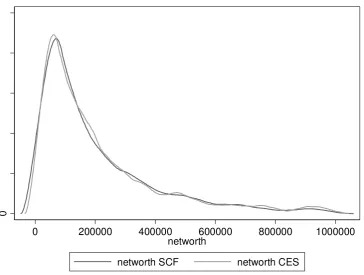
Figure 2: Household net wealth kernel distribution, 2004

0

0 200000 400000 600000 800000 1000000

NETWORTH

networth SCF networth CES

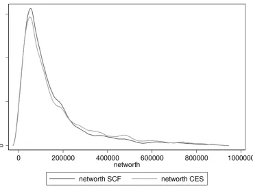
Figure 3: Household net wealth kernel distribution, 2001

0

0 200000 400000 600000 800000 1000000

networth

networth SCF networth CES

Source: SCF and CES 1989-2007, own computations.

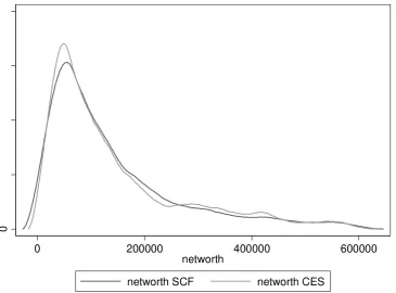
Figure 4: Household net wealth kernel distribution, 1998

0

0 200000 400000 600000 800000 1000000

networth

networth SCF networth CES

Figure 5: Household net wealth kernel distribution, 1995

0

0 200000 400000 600000 800000 1000000

networth

networth SCF networth CES

Source: SCF and CES 1989-2007, own computations.

Figure 6: Household net wealth kernel distribution, 1992

0

0 200000 400000 600000 800000 1000000

networth

networth SCF networth CES

Figure 7: Household net wealth kernel distribution, 1989

0

0 200000 400000 600000

networth

networth SCF networth CES

Source: SCF and CES 1989-2007, own computations.

Figure 8. Ratio of net wealth over income over the life cycle – cohort averages. Each line

corresponds to a different cohort.

Figure 9. Ratio of non durables consumption over income over the life cycle – cohort averages.

Each line corresponds to a different cohort.

Tables

Table 1: correlations between logarithmic income and the wealth (SCF) variables

2007 2004 2001 1998

SCF CES SCF CES SCF CES SCF CES

fin 0.26*** 0.16*** 0.26*** 0.18*** 0.27*** 0.14*** 0.22*** 0.11**

nfin 0.27*** 0.30*** 0.25*** 0.26*** 0.24*** 0.18*** 0.19*** 0.17***

asset 0.32*** 0.29*** 0.30*** 0.26*** 0.31*** 0.20*** 0.25*** 0.17***

debt 0.46*** 0.43*** 0.41*** 0.40*** 0.47*** 0.42*** 0.38*** 0.29***

networth 0.30*** 0.26*** 0.28*** 0.23*** 0.29*** 0.18*** 0.23*** 0.16***

kgtotal 0.21*** 0.21*** 0.18*** 0.15*** 0.18*** 0.09** 0.13*** 0.12**

1995 1992 1989

SCF CES SCF CES SCF CES

fin 0.18*** 0.12** 0.24*** 0.19*** 0.25*** 0.08***

nfin 0.20*** 0.09** 0.16*** 0.09*** 0.21*** 0.10***

asset 0.24*** 0.12*** 0.21*** 0.11*** 0.27*** 0.13***

debt 0.32*** 0.29*** 0.28*** 0.14*** 0.39*** 0.33***

networth 0.22*** 0.10*** 0.19*** 0.10*** 0.25*** 0.12***

kgtotal 0.14*** 0.04** 0.12*** 0.07*** 0.15*** 0.06***

Table 2. Number of households in the dataset, by date of birth and year of survey

Date of birth of household and cohorts

Oldest: 19- 1898 02 06 10 14 18 22 26 30 34 38 42

Youngest: 19- 01 05 09 13 17 21 25 29 33 37 41 45

Cohort: -> 1 2 3 4 5 6 7 8 9 10 11 12

1989 57 89 181 270 341 411 442 385 363 409 467 519

1992 0 98 147 231 333 390 434 371 340 365 411 559

1995 0 36 91 151 224 364 350 392 330 337 373 482

1998 0 39 48 0 565 297 413 443 479 418 417 519

2001 0 0 0 0 0 99 414 494 511 515 521 653

2004 0 0 0 0 0 696 221 512 521 599 692 825

2007 0 0 0 0 0 484 81 396 433 463 521 687

Oldest: 19- 46 50 54 58 62 66 70 74 78 82 86

Youngest: 19- 49 53 57 61 65 69 73 77 81 85 89

Cohort: -> 13 14 15 16 17 18 19 20 21 22 23

1989 736 732 774 809 688 405 138 0 0 0 0

1992 651 775 828 780 744 577 439 21 0 0 0

1995 626 697 696 794 725 584 468 248 0 0 0

1998 724 816 842 863 843 788 739 550 268 0 0

2001 866 942 983 1107 1079 966 905 723 662 165 0

2004 990 1131 1227 1255 1226 1121 1020 890 770 628 81

Table 3: equation (2), specification 1 (gross wealth) - two different dependent variables

Total consumption Non durables consumption

Expl. variables Coeff. Standard error Coeff. Standard error

income 0.552*** 0.046 0.481*** 0.044

fin -0.031 0.019 -0.034* 0.018

house 0.022** 0.011 0.039*** 0.010

ore 0.020 0.019 0.021 0.018

old*income -0.011 0.044 -0.021 0.042

old*fin 0.051 0.033 0.021 0.032

old*house 0.007 0.033 0.025 0.031

old*ore -0.045 0.029 -0.020 0.027

age 0.017** 0.009 0.017** 0.008

agesq -0.000* 0.000 -0.000 0.000

educ 0.145** 0.059 0.044 0.054

not working -0.031 0.097 -0.133 0.092

race-black 0.174 0.320 0.185 0.304

race-other -1.910*** 0.577 -1.974*** 0.566

Note: All the fixed effects estimations were carried out using the Repeated Imputation Inference (RII) , using all the

five implications resulting from the CES procedure of imputing missing income values. ***, **, * significant at 1, 5,

10% respectively; standard errors are clustered (Petersen 2009).

Table 4: equation (2), specification 2 (net financial wealth) - two different dependent variables

Total consumption Non durables consumption

Expl. variables Coeff. Standard error Coeff. Standard error

income 0.546*** 0.049 0.466*** 0.046

netfin -0.007 0.005 -0.008* 0.005

house 0.008 0.012 0.025** 0.011

ore 0.022 0.019 0.023 0.018

old*income 0.010 0.036 -0.018 0.035

old*netfin 0.023** 0.010 0.021 0.032

old*house 0.022 0.031 0.034 0.030

old*ore -0.043 0.028 -0.019 0.027

age 0.019** 0.009 0.019** 0.008

agesq -0.000** 0.000 -0.000 0.000

educ 0.090* 0.054 -0.007 0.051

not working -0.009 0.098 -0.116 0.093

race-black 0.109 0.322 0.113 0.307

race-other -2.024*** 0.596 -2.078*** 0.590

Note: All the fixed effects estimations were carried out using the Repeated Imputation Inference (RII) , using all the

five implications resulting from the CES procedure of imputing missing income values. ***, **, * significant at 1, 5,

Table 5: equation (2), specification 3 (net tangible wealth) - two different dependent variables

Total consumption Non durables consumption

Expl. variables Coeff. Standard error Coeff. Standard error

income 0.617*** 0.034 0.555*** 0.033

fin -0.023 0.020 -0.020 0.019

nettng 0.010 0.006 0.018*** 0.007

old*income -0.060 0.042 -0.049 0.040

old*fin 0.054 0.033 0.031 0.033

old*nettng 0.012 0.026 0.023 0.025

age 0.019*** 0.007 0.027*** 0.007

agesq -0.000*** 0.000 -0.000*** 0.000

educ 0.121** 0.059 0.012 0.055

not working -0.045 0.094 -0.099 0.090

race-black 0.180 0.331 0.181 0.322

race-other -1.718*** 0.581 -1.739*** 0.582

Note: All the fixed effects estimations were carried out using the Repeated Imputation Inference (RII) , using all the

five implications resulting from the CES procedure of imputing missing income values. ***, **, * significant at 1, 5,