Assessing the quality of institutions’
rankings obtained through multilevel
linear regression models
Arpino, Bruno and Varriale, Roberta
Dodena Research Centre - Università Bocconi
2009
Online at
https://mpra.ub.uni-muenchen.de/19873/
DONDENA WORKING PAPERS
Assessing the quality of institutions’ rankings obtained
through multilevel linear regression models
Bruno Arpino, Roberta Varriale
Working Paper No. 19
URL: www.dondena.unibocconi.it/wp19
July 2009
Carlo F. Dondena Centre for Research on Social Dynamics Università Bocconi, via Guglielmo Röntgen 1, 20136 Milan, Italy
http://www.dondena.unibocconi.it
The opinions expressed in this working paper are those of the author and not those of the Dondena Centre which does not take an institutional policy position.
models
Bruno Arpino
Department of Decision Sciences and “Carlo F. Dondena” Centre for Research on Social Dynamics
Università Bocconi via Guglielmo Röntgen 1
20136 Milan Italy
Roberta Varriale
Department of Methodology and Statistics Tilburg University
PO Box 90153 5000 LE Tilburg The Netherlands
and
Dipartimento di Statistica Università di Firenze
Viale Morgagni 59 50134 Firenze
Italy
Abstract
The aim of this paper is to assess the quality of the ranking of institutions obtained with multilevel techniques in presence of different model misspecifications and data structures. Through a Monte Carlo simulation study, we find that it is quite hard to obtain a reliable ranking of the whole effectiveness distribution while, under various experimental conditions, it is possible to identify institutions with extreme performances. Ranking quality increases with increasing intra class correlation coefficient and/or overall sample size. Furthermore, multilevel models where the between and within cluster components of first-level covariates are distinguished perform significantly better than both multilevel models where the two effects are set to be equal and the fixed effect models.
Keywords
1. Introduction
In recent decades, there has been an increasing use of performance indicators in the form of rankings or “league tables” in many areas of public sector, such as educational, health and socio-economic fields, with the aim of comparing the effectiveness of public institutions.
Traditionally, performance indicators based on “raw” measures have been used to depict comparative performance in sport and commerce and their extension to ranking of services provided by public institutions has attracted resistance and criticism (Adab et al., 2002). Nowadays, it is widely recognized that raw rankings can be misleading (Goldstein and Spiegelhalter, 1996). First of all, simple league tables ignore the quantification of uncertainty associated with the rankings. Secondly, it should be recognized that the institutions’
performances depend not only on the characteristics of the institutions themselves but also on those of their components. As an example, in the educational context, schools’ performance is obviously affected by students’ socio-economic background: schools with more problematic students tend to perform worse than schools serving advantaged students. Therefore, in order to make valuable comparisons among institutions, it is important to use some “net” measures that adjust for the so-called “compositional cluster effect”.
The general approach to obtain such adjustment is through regression analysis using an indicator of effectiveness as the dependent variable, while the characteristics of the
institutions and those of their components are included as covariates (see, e.g., Tekwe et al., 2004). Within this general approach, multilevel models have become a widely accepted approach because they explicitly recognize the hierarchical structure of the data (individuals clustered within institutions) and overcome the inadequate assumption of independence among units belonging to the same institution, typical of standard models (Snijders and Bosker, 1999). Examples of applications of multilevel regression models can be found in many disciplines, such as medicine (Hofer et al, 1996; Normand et al, 1997) and poverty analysis (Aassve and Arpino, 2007).
An important field for which multilevel modelling techniques offer particularly fruitful application is educational research, where the focus is usually on the assessment of schools’ or universities’ performances. In this context, the necessity to evaluate the effectiveness of the institutions was originally justified on two distinct grounds: accountability and school choice (Leckie and Goldstein, 2009). The former aims at increasing the quality of the educational system and the latter at providing useful information for the choice of the future school for a child. With reference to the general problem of ranking schools, the seminal work by Aitkin and Longford (1986), subsequently discussed by Goldstein et al. (1993), describes the advantage of using multilevel regression models compared to the one-level models. Subsequently, many other applied works in the same context of analysis have used similar methodologies (see, e.g., Raudenbush and Willis, 1995; Rampichini et al, 2004; Chiandotto and Varriale, 2005; Jürges and Sneider, 2007; Wößmann, 2008).
As described by Goldstein and Spigelhalter (1996), in a two-level model, e.g. with students nested within schools, the second level residuals can be interpreted as a measure of the school effectiveness with respect to the given outcome net of the effect of the covariates and they can be used to evaluate and rank the schools. The choice of the specific outcome as well as
The quality of the ranking obtained through multilevel models depends on the validity of the assumptions underlying the multilevel regression model. These are similar to those used in ordinary multiple regression analysis, such as homoscedasticity and normal distribution of the residuals. While some Monte Carlo simulation studies have been carried out in order to evaluate the robustness of multilevel models with respect to the parameter estimates and standard errors in case of violations of these assumptions (see, e.g., Maas and Hox, 2004), we focus on the effect of different model misspecifications on the ranking quality. Furthermore, we assess the role of the data structure (cluster size and number of clusters) and of the intra-class correlation coefficient (ICC). Finally, we evaluate and discuss the consequences of assuming that the between and within effects of the level-1 covariates are equal, as implicitly done in many applied works. In our work, we focus in particular on the ability of multilevel models to identify extreme performing institutions, which usually are the most interesting for researchers and policy makers.
Recent works have focused on empirical comparison among different modelling approaches for value-added assessment. For example, Tekwe et al (2004) and Jürges and Schneider (2007) compared the rankings obtained with different model specifications. Ladd and Walsh (2002) discussed different fixed effects models, focusing in particular on the impact of
measurement error on the ranking of schools. They found that the ranking is not always robust to the choice of the model and covariates to adjust for. In our simulation, we use a different perspective. In particular, we compare the estimated ranking with the generated (true) one in the presence of different model misspecifications and we evaluate if these model
misspecifications affect the ranking quality. Moreover, to the best of our knowledge, the implication of having different between and within covariate effects did not receive the attention it deserves.
Another interesting work assessing the quality (in terms of uncertainty) of rankings obtained through multilevel models has been presented by Lockwood et al (2002). In their work, the authors focused on the Bayesian perspective, while we use a frequentist approach.
The paper is structured as follows: in section 2 we provide a brief overview of the multilevel linear model and the mostly used methods to obtain the estimates of higher level residuals; in section 3 we describe our simulation study and in section 4 we present the results; section 5 concludes the work with a discussion and concluding remarks.
2. Ranking of clusters in multilevel linear regression
models
In this paper, the problem of schools’ ranking will be used as an illustrative example. Let Yij
be a performance indicator, such as a test result, measured on student i attending schools j, for
i=1,…,nj and j=1,…,J. Our aim is to rank the schools with respect to the performance
indicator in order to identify and reward the best-performing institutions.
In order to rank the schools, we could simply use the schools’ average performance indicator,
j
Y , as usually done with “league tables”. However, the consequent raw ranking does not take
As introduced above, a general approach to obtain such adjustment is through regression analysis, with both a fixed and a random approach, having Yij as dependent variable, while the
characteristics of the institutions and those of their components are included as covariates. To illustrate how it is possible to derive a ranking of schools that adjust for student characteristics using multilevel techniques, we will consider a simple example of a random intercept linear regression model with two level-1 covariates1:
Yij = α + β1 TOT X1ij + β2TOT X2ij + eij + uj (1)
where X1ij and X2ij are level-1covariates, β1TOT andβ2TOT are the regression coefficients
measuring the total effect of the covariates on the outcome variable, and eij and uj are the
level-1 and level-2 errors. Just to give a simple example, Tekwe et al. (2004) used as covariates the minority and poverty status of students.
The usual assumptions of multilevel linear regression models are: exogenous covariates, uncorrelated errors, normality and homoscedasticity of the level-1 and level-2 error distributions (Skrondal and Rabe-Hesketh, 2004).
As noticed for example by Neuhaus and Kalbfleisch (1998) and Snijders and Bosker (1999), in a multilevel context, the relationships at the cluster level, measured by the between-cluster effects, can be very different from the relationships at the micro level, measured by the within-cluster effects. The regression model (1) mixes the two relationships and its estimated total regression coefficients βrTOT are an average of the between-cluster and the within-cluster
effects.
From model (1) we can obtain purely between-schools (βB) effects of the covariates aggregating the response and exploratory variables at the school level:
j j j B j B
j X X e u
Y 1 1 2 2 . (2)
In this model, all the information on the within-schools variability is ignored. If we are interested exclusively on the within-schools effects (βW), we can subtract model (2) from (1), obtaining:
ij j
ij j
W j ij W j
ij Y X X X X e e
Y 1 1 1 2 2 2 . (3)
The same within-school estimates can be obtained by replacing the random effect uj in (1)
with a fixed intercept αj (Rabe-Hesketh and Skrondal, 2005):
1 1 2 2
W W
ij ij ij j ij
Y X X e . (4)
In order to simultaneously estimate both the between and within-cluster effects, we can combine models (2) and (3):
1 1 1 1 1 2 2 2 2 2
W B W W B W
ij ij j ij j ij j
Y
X
X
X
X e u . (5)1
When the within and between effects are equal for each covariates, βrB =βrW (r=1,2), the
models (5) and (1) are equivalent. Therefore, model (1) can be considered as a special case of model (5).
To derive a ranking of schools using a two-level model with students clustered into schools we can give a value-added interpretation to the models we introduced above. In random effects models (1) and (5), the level-2 residuals, uj, can be interpreted as a measure of the
residual effect of the schools on the outcome variable measured at student level, after the effect of the independent variables included in the model has been controlled for. Through the ranking of the errors uj we obtain our ultimate goal, which is the ranking of schools j. There
are two methods commonly used to assign values to uj: the maximum likelihood estimation
and the EmpiricalBayes prediction2, that treat uj, respectively, as an unknown fixed
parameter and as a random variable (Snijders and Bosker, 1999).
Let us now define the total residuals for models (1) and (5) as ξij = eij + uj and the predicted
errors, ˆ , as ij ˆij Yij Yˆij. The ML estimates of uj, in a two-level random intercept model,
can be obtained as the sample mean of ˆ for each cluster (Skrondal and Rabe-Hesketh, ij 2004):
1 1
1 ˆ 1 ˆ ˆ
ˆ .
j j
n n
ML
j ij ij ij j ij
i i
j j
u Y Y Y Y
n n
. (6)The Empirical Bayes predictions uˆEBj are obtained as the mean value of the posterior distribution of uj, where the prior is usually a normal distribution with mean of zero and the
estimated variance of uj plugged in (Rabe-Hesketh and Skrondal, 2005).
In two-level random intercept linear models there is a simple relationship between the estimates obtained with these two approaches: uˆEBj sˆj*uˆMLj , where sˆj= τ2 / (τ2+ σ2/ nj) is
the so-called shrinkage factor that ranges from 0 to 1 and causes the empirical Bayes
prediction to be shrunken toward 0. When the data structure is balanced (constant number of first-level units in each cluster) the values assigned by the two methods to uj are equal up to a
constant and, as a consequence, the rankings of uˆ (and of j j) are the same. However, even when the data structure is unbalanced, Tekwe et al (2004) found little impact of shrinkage by itself on value-added assessment of school performance. Since we will use a Monte Carlo simulation study based on balanced data structures, we will only focus on ML estimates of uj
and we will refer to these simply as uˆ , instead of j ML j
uˆ .
From (6), we can interpret the uˆ as an “adjustment” of the average outcome j Yj observed in
cluster j with the quantity Yˆ that depends on the model specifications. Models in equations (1) and (5), having different covariates specifications, “adjust” Yj in a different way and this has consequences on the ranking of uˆ . j
2
From the model in equation (1), we have:
1 1 2 2
ˆ TOT TOT
j j j j
u Y
X
X . (7)and from the model in equation (5), we have:
1 1 2 2
ˆ B B
j j j j
u Y X X . (8)
The uˆ obtained from the two models are equal when j βrW =βrB (r =1,2); otherwise, the model
in equation (5) correctly uses the between-cluster effects βr B as weights for the between
component of the covariates, Xrj, while the weights used by model (1) are the total effects.
From model (4), we can interpret the fixed effects αj in a similar way:
1 1 2 2
ˆ W W
j Yj X j X j
. (9)If βrW =βrB, this model gives exactly the same ranking as the models in equations (1) and (5).
Otherwise, βrTOT can be expressed as an average of βrW and βrB, weighted in inverse proportion
to their respective variances (Maddala, 1971) and, interestingly, the more similar (different) the clusters are in terms of cluster-level averages of level-1 covariates the more similar βrTOT
will be to the βrW (βrB). This implies that the more similar the clusters are in terms of cluster
means the more similar the ranking obtained through adjustments (7) and (9). On the contrary, in the presence of very different clusters, adjustments (7) and (8) will be more similar with respect to those based on (9).
Summarising, we expect substantial differences in the rankings obtained using models (1), (4) an (5) only in presence of a discrepancy in the between and within-cluster effects of the covariates. Moreover, these differences should be small when the difference among the two effects is small.
3. Simulation procedure
In this section we illustrate the Monte Carlo simulation study we used in order to evaluate the goodness of schools’ rankings obtained with multilevel models. In particular, we aim at evaluating the consequences of different model misspecifications concerning the cluster-level errors and data features (data structure, ICC value, discrepancy among the between and within effects of the level-1 covariates) and at comparing the performance of a fixed effect model in comparison with the multilevel models. In this work we concentrate on the assumptions of normality and homoscedasticity of cluster-level errors and we assess the effects produced by their violation on the quality of cluster ranking. We focus on model misspecifications relative to level-2 residuals since the sample size at the second level is always lower than the sample size at level-1, implying that the assumptions on errors at the highest level are more
problematic.
1. we generate the data representing the schools’ performance through a multilevel linear regression model with different types of distribution of the level-2 error term, uj;
2. we obtain the true ranking of uj (and j) for each true distribution of uj;
3. we estimate the model parameters through three different estimation methods; 4. for each estimation method we obtain, as explained in section 2, the maximum
likelihood estimates of uj (uˆj), and we rank them (and, consequently, we rank the
clusters j);
5. for each estimation method, we compare the true and estimated rankings of uj.
Steps 1 and 2
As the first step of our simulation study, we generate two-level balanced data structures, where the overall sample size N is determined by the product of the number of clusters, nc, and the fixed cluster size, cs. In the data generating model we use two level-1 covariates, X1
and X2, which are allowed to vary both within and between clusters. In particular, they are
treated as random variables and are generated through a variance component model as the sum of two independent normal variables representing their within (XW) and between components (XB ):
, 1, 2
W B kij kij kj
X X X for k . (10)
where it is assumed that:
2
. 1) are with mean and variance , for =1,2
k k
B
kj X X
X X iid k
2
. 2) are with zero mean and variance , for =1,2
k W
kij X
X X iid k
. 3) kjB Wkij, , and for =1,2
X X X i j k .
The data generating model is then:
1 1 1 1 2 2 2 2
W W B B W W B B
ij ij j ij j ij j
Y X X X X e u . (11)
where α and β are the model parameters and eij and uj are the error terms defined, respectively,
at level 1 and level 2.
Obviously, the true between (XkjB) and within components (XkijW) of the covariates in equation (10) are not observable in practice and can be distinguished in an estimation model by using
their sample counterparts (see, i.e., equation (5)), the cluster mean
1 1 = for j n B
kj kij kj
i j
X X X n
, and
the deviation from the cluster mean (centred covariate) X~kij XkijXkij for XkijW.
We use five different processes to generate the “true” distribution of the error terms uj:
a. homoscedastic, Normal(N.Hom);
b. heteroscedastic, Normal (N.Het);
c. homoscedastic, asymmetric (Chi-Square with one degree of freedom, CHI);
d. homoscedastic, symmetric and bimodal (50:50 mixture of two normal
distributions, BIM);
The first specification (a) conforms to the usual assumptions; the other four imply different forms of model misspecification when the normality and homoscedasticity assumptions are used in the estimation procedure. In all cases, the values sampled from the assumed
distribution of uj are used to obtain the true ranking of j, are indicated with RTj.
Besides the error term distribution, three other conditions have been varied: (i) number of clusters (nc = 30, 50, 100), (ii) cluster size (cs = 5, 30, 50) and (ii) the intraclass correlation
coefficient value, 2 2 2
, (ρ= 0.1, 0.2, 0.3); as mentioned by Maas and Hox (2004), these
values are commonly found in the applied educational literature. The residual variance at level 2 is determined as a consequence of the imposed values of ρ and of the residual variance at level 1, which is set to 0.5. The intercept term α in equation (6) is set to 0; the other
regression coefficients are set to 1, except 1B that is set to 1.5: in this way, the between and the within effects of the first covariate are different. Finally, since we also want to evaluate the consequences of assuming the equality of the covariates’ between and within effects, we run a set of simulations where the difference between the two effects for both covariates is varied and take values -1; 0 and +1.
Steps 3 and 4
In order to estimate the model parameters and subsequently obtain the ranking of uj, we use
and compare three different estimation models:
M1. B j ij j
j W j B j W
ij X X X X e u
Y 1 ~1 1 1 2 ~2 2 2
M2. 1TOT 1 2TOT 2
ij ij ij ij j
Y X X e u
M3. 1 1 2 2
1
J
W W
ij ij ij j j ij j
Y X X D e
The characteristics of the three models have been discussed in section 2. M1 and M2 are two-level models corresponding to equations (5) and (1). M3 is a fixed effect model corresponding to equation (4).
Each model is used to obtain the estimates of the cluster effects uj and, consequently, the
estimated ranking of j (REj); M1 and M2 by means of the maximum likelihood estimates of uj
and M3 by means of the estimated αj coefficients. In the estimation of Models M1 and M2 we
make the usual assumptions on the error terms (section 2) and, therefore, these models are misspecified if the true uj distribution is not normal and/or not homoscedastic (cases from
b.-e.). In this case, we aim at assessing the implications on the ranking quality of these misspecifications by comparing M1 and M2 with respect to model M3. Moreover, as we explained in section 2, the ranking obtained through the three models is expected to be different if βr W and βr B (r=1,2) coefficients are different.
Step 5
As the last step of our Monte Carlo experiment, we evaluate the quality of the estimated rankings obtained with different model conditions comparing the closeness of REj (estimated
For each experimental condition we generate 1000 simulated data sets and we evaluate two measures of the ranking quality. As a first measure, we calculate the average Spearman correlation coefficient between the true and the estimated distribution of the level-2 residuals over the 1000 simulated data sets. For each replication, the coefficient is calculated as:
1 , 2 6 1 1 j j T E J T E j R R R R J J
, 1, 2
W B kij kij kj
X X X for k
where J is the total number of clusters; ρRT,RE ranges from -1 to +1 and the closer it is to 1, the
more similar the rankings are. The average Spearman correlation coefficient, ρ, also ranges from -1 to +1 and shows how well a model performs in the classification of the level-2 units.
The Spearman correlation coefficient is an overall measure and is affected by the difference between the estimated ranking positions of each unit with respect to the true positions. A property of the index is that the impact of a misclassification increases quadratically with the distance between the true and estimated position and only the absolute value of this distance matters. For example, consider the ranking of school j out of 100 schools. Consider the two situations with RTj =100; REj =90 and RTj = 50; REj = 40: in both cases, the mistake in the
classification of school j has the same weight in the index, even if the two mistakes can be considered different from a substantive point of view. In the first case a school with an extreme performance is ranked 10 positions below and this could make a difference in the assignment of a price or a sanction; in the second case, it probably makes little difference for school j to be ranked in the 50th or 40th position.
In order to evaluate the quality of the estimated ranking separately for groups of institutions we introduce classification matrixes. The idea is to divide the true and the estimated
distributions of uj into intervals defined by the deciles of the respective distributions and to
evaluate, for each interval, the percentage of correctly classified schools over the 1000 simulated data sets.
Following the example introduced above (section 2), it is natural to divide the schools into two groups: “Top” and “Non Top”. In particular, we define the “Top” institutions (best-performing) as those belonging to the last3 decile of the true distribution of uj and we define
the remaining institutions as “Non Top”4. In this setting, two kinds of errors can be generated in the ranking: one error involves classifying as Top a true Non Top institution (γ), and the other error involves classifying as Non Top a true Top institution (δ):
γ= Pr(TE/NTT),
δ= Pr(NTE/TT).
3
Whether the Top institutions belong to the first or last decile of the true distribution of uj depends on the nature
of the observed outcome Yij. When Yij represents some “positive” phenomenon, such as a test result or salary in
first job, the Top institutions belong to the last decile. On the contrary, if Yij represents some “negative”
phenomenon such us the school dropout rate, the Top institutions belong to the first decile.
4
Which is the worse error strictly depends on the aim of the research or on the policy goals. In our example, where a public organisation wants to reward the best-performing schools, the overriding concern is misclassifying schools as Top when, in fact, they are not. This is mainly because a Non Top school will become an example for the others and will receive an
undeserved reward. In this case the public evaluator would be more concerned to reduce error
γ. In other situations a public evaluator could be more interested in reducing errors of type δ or both.
Similar to Lockwood et al. (2002), we think that if policy makers intend to use the rankings for accountability, it is advisable that the choice between focusing on γ or δis guided by consideration of the losses incurred by these different kinds of errors. For example, if schools identified as extreme are likely to face punitive sanctions or receive large monetary rewards, then policy makers might find misclassifying non extreme schools as relatively more costly and prefer using decision rules based on γ; if schools classified as low-performing will receive additional resources, then policy makers might see missed investments as costly and prefer using decision rules based on minimising δ.
In the following, we will focus only on error γto illustrate the results of our simulation study.
4. Results
In the first set of simulations, we consider different uj distributions, estimation methods and
combinations of cluster size (cs) and number of clusters (nc), while we set the Intraclass Correlation Coefficient (ICC) at a medium level (0.2).
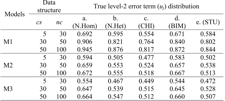
Table 1 shows the Spearman correlation coefficient averaged over 1000 replications. Taking the uj distribution into account, the best scenario, regardless of the estimation model, is a.,
when the level-2 error term distribution is correctly specified (normal and homoscedastic). On the contrary, the worst scenario is always (c.), when the uj are generated from a Chi-Square
[image:13.612.119.495.504.673.2]distribution.
Table 1.Spearman correlation coefficient (averaged over 1000 replications) for different estimation models, data structure and uj distributions
Models
Data
structure True level-2 error term (uj) distribution
cs nc a.
(N.Hom)
b. (N.Het)
c. (CHI)
d.
(BIM) e. (STU)
M1
5 30 0.692 0.595 0.554 0.671 0.584 30 50 0.906 0.821 0.764 0.840 0.802 50 100 0.945 0.876 0.817 0.872 0.844
M2
5 30 0.594 0.505 0.477 0.583 0.502 30 50 0.659 0.553 0.524 0.657 0.538 50 100 0.672 0.555 0.518 0.667 0.513
M3
5 30 0.554 0.467 0.449 0.544 0.472 30 50 0.647 0.539 0.515 0.645 0.528 50 100 0.664 0.547 0.512 0.660 0.507
Focusing on the different estimation methods, M1, by allowing βrWto be different fromβrB
(r=1,2), performs better than M2 and M3. For all estimation methods, the Spearman
combination of cs=50 and nc=100. In particular, even for the worst scenario (case c.), the ranking quality seems to be acceptable when using model M1 for the estimation process and the sample size is not small. For example, with a medium sample size (N = 1500; cs = 30 and
nc = 50) the Spearman coefficient is equal to 0.764 while with a big sample size, cs = 50 and
nc = 100, the index is 0.817.
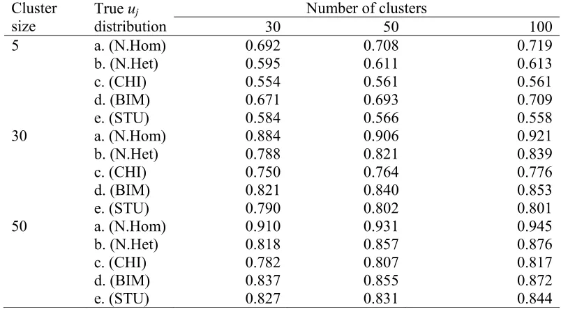
[image:14.612.104.506.250.472.2]Table 2 shows the analysis of the data structure effect on ranking quality. From this table we see that ranking quality increases as the values of cs or nc increase. However, the values of the Spearman correlation coefficient are very similar if we consider two data structures with the same sample size (N=1500) but different number of clusters and cluster size (cs = 30; nc = 50 and cs = 50; nc = 30).
Table 2. Spearman correlation coefficient (averaged over the 1000 replications) for different data structures and uj distributions with estimation model M1
Cluster size
True uj
distribution
Number of clusters
30 50 100
5 a. (N.Hom) 0.692 0.708 0.719
b. (N.Het) 0.595 0.611 0.613
c. (CHI) 0.554 0.561 0.561
d. (BIM) 0.671 0.693 0.709
e. (STU) 0.584 0.566 0.558
30 a. (N.Hom) 0.884 0.906 0.921
b. (N.Het) 0.788 0.821 0.839
c. (CHI) 0.750 0.764 0.776
d. (BIM) 0.821 0.840 0.853
e. (STU) 0.790 0.802 0.801
50 a. (N.Hom) 0.910 0.931 0.945
b. (N.Het) 0.818 0.857 0.876
c. (CHI) 0.782 0.807 0.817
d. (BIM) 0.837 0.855 0.872
e. (STU) 0.827 0.831 0.844
From these results we conclude that increasing the total sample size substantively improves the quality of the ranking, while the composition of the sample (combination of cs and nc) does not have a strong effect per se.
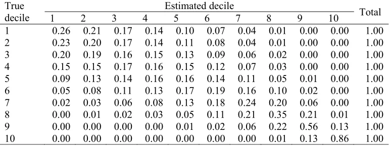
Tables 3a and 3b show two classification matrixesobtained for a total sample size equal to 3000 (cs = 30 and nc = 100) with the correct model specification M1. In the first table, the true uj distribution is normal and homoscedastic (case a., best scenario, as summarized in
Table 1), while in the second table the true uj distribution is Chi-Square (case c., worst
scenario). To ease the interpretation of the classification matrixes, let us give some examples. In the first row of Table 3a we have the relative conditional frequencies of the institutions that belong to the first decile of the true distribution and are classified in the different estimated ten groups. Therefore, we can interpret the first cell as the percentage of correctly classified first group institutions: the probability that one institution is estimated as belonging to the first group given that it belongs to the first group of the true uj distribution. The second cell
Table 3a. Classification matrix for estimation model M1 and a normal and homoscedastic uj
distribution (case a.) with cs = 30 and nc = 100 True
decile
Estimated decile
Tot. 1 2 3 4 5 6 7 8 9 10 1 0.73 0.22 0.05 0.01 0.00 0.00 0.00 0.00 0.00 0.00 1.00 2 0.21 0.41 0.24 0.09 0.03 0.01 0.00 0.00 0.00 0.00 1.00 3 0.05 0.24 0.33 0.23 0.10 0.04 0.01 0.00 0.00 0.00 1.00 4 0.01 0.09 0.23 0.28 0.22 0.12 0.04 0.01 0.00 0.00 1.00 5 0.00 0.03 0.10 0.23 0.27 0.21 0.11 0.04 0.01 0.00 1.00 6 0.00 0.01 0.04 0.11 0.22 0.27 0.22 0.11 0.03 0.00 1.00 7 0.00 0.00 0.01 0.04 0.11 0.22 0.28 0.23 0.09 0.01 1.00 8 0.00 0.00 0.00 0.01 0.04 0.11 0.23 0.32 0.24 0.04 1.00 9 0.00 0.00 0.00 0.00 0.01 0.03 0.10 0.24 0.42 0.21 1.00 10 0.00 0.00 0.00 0.00 0.00 0.00 0.01 0.04 0.21 0.74 1.00
Table 3b. Classification matrix for estimation model M1 and a Chi-Square uj distribution (case c.) with
cs = 30 and nc = 100 True
decile
Estimated decile
Total 1 2 3 4 5 6 7 8 9 10 1 0.26 0.21 0.17 0.14 0.10 0.07 0.04 0.01 0.00 0.00 1.00 2 0.23 0.20 0.17 0.14 0.11 0.08 0.04 0.01 0.00 0.00 1.00 3 0.20 0.19 0.16 0.15 0.13 0.09 0.06 0.02 0.00 0.00 1.00 4 0.15 0.15 0.17 0.16 0.15 0.12 0.07 0.03 0.00 0.00 1.00 5 0.09 0.13 0.14 0.16 0.16 0.14 0.11 0.05 0.01 0.00 1.00 6 0.05 0.08 0.11 0.13 0.17 0.19 0.16 0.10 0.02 0.00 1.00 7 0.02 0.03 0.06 0.08 0.13 0.18 0.24 0.20 0.06 0.00 1.00 8 0.00 0.01 0.02 0.03 0.05 0.11 0.21 0.35 0.21 0.01 1.00 9 0.00 0.00 0.00 0.00 0.01 0.02 0.06 0.22 0.56 0.13 1.00 10 0.00 0.00 0.00 0.00 0.00 0.00 0.00 0.01 0.13 0.86 1.00
The sum of the conditional frequencies in cells 2 to 10 measures the percentage of
misclassified first group institutions. The further we are from the first cell, the more serious the misclassification is. Extending the interpretation to the whole matrix, we can say that the diagonal includes the percentage correct classification for each of the ten deciles of the true distribution; in the other cells we find the percentages for all possible misclassifications whose severity increases as we move away from the diagonal. As expected, the highest values are on the diagonal and the “strong-misclassification cells” (the furthest from the diagonal) show very small percentages. For example, the first row of Table 3a shows that, out of the clusters belonging to the first interval of the true distribution of uj, 73% are correctly
classified in the first decile, while 22% and 5% are wrongly classified since they belong, respectively, to the second and third interval of the estimated distribution of uˆ . A very j interesting result is that extreme institutions, those belonging to the first and tenth decile of the true uj distribution, show the highest percentages of correct classification, as shown in
cells (1,1) and (10,10). This result is particularly important for practitioners because as we already mentioned they are usually interested in identification of the “extreme” institutions.
This result is also consistent with the literature which states that only extreme performances turn out to be significantly different from the others because of the prediction error variability (Goldstein and Spieghelter, 1996).
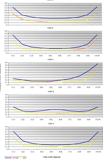
[image:15.612.114.500.273.418.2]1 shows the values on the diagonal of the classification matrixes obtained for the three estimation models and different uj distributions with cs = 30, nc = 100. Regardless of the uj
[image:16.612.133.482.126.662.2]distribution, the best performing estimation method in terms of ranking quality is always M1.
This result is especially interesting in terms of the comparison of M1 and M3: when the within-between covariates effects are different, even if the true uj distribution is far away from
normality, the random effects approach performs better that the fixed effects approach in estimating the higher level units effects. However, even with M1, while the percentages in cells (1,1) and (10,10) are quite high (higher than 0.7) for case a. (homoscedastic, Normal uj
distribution), b. (heteroscedastic, Normal uj distribution) and e. (homoscedastic, symmetric
and heavy-tailed uj distribution), they are quite low for case d. (homoscedastic, symmetric and
bimodal uj distribution). When the true distribution of uj is Chi-Square (case c.), the
classification errors in the two tails are very different: the uj in the highest positions are quite
well classified, while the percentage of correct classification is low for the left-most cell (1,1). This is, of course, due to the positive skewed nature of the Chi-square distribution. In case d. the uj in the middle of the true distribution are slightly better classified compared to what
happens with the other distributions.
In Table 4 we summarise the classification matrix by distinguishing only Top (last decile) and Non-Top schools (the rest). The table shows the two error probabilities introduced in section 3, γ = Pr(TE/NTT) and δ = Pr(NTE/TT) and their complement to 1, 1-γ = Pr(NTE/NTT) and1-δ
= Pr(TE/TT),that measure the probabilities of correct classification. As found before, the
models M2 and M3 show very similar classification performances, and M1 is the best estimation model, having the highest correct classification probabilities, Pr(TE/TT),
Pr(NTE/NTT), and correspondingly, the lowest misclassification probabilities, Pr(NTE/TT) and
Pr(TE/NTT). The effectiveness of M2 and M3 is rather low in terms of 1-δwhile their
[image:17.612.95.511.419.475.2]performances are still quite satisfactory in terms of γ.
Table 4. Conditional probabilities γ =Pr(TE/NTT), 1-γ = Pr(NTE/NTT), , δ = Pr(NTE/TT) and
1-δ = Pr(TE/TT) for different estimation models, uj normal and homoscedastic, cs=30 and
nc=100
Models γ =Pr(TE/NTT) 1-γ = Pr(NTE/NTT) δ = Pr(NTE/TT) 1-δ = Pr(TE/TT)
M1 0. 029 0.971 0.261 0.739
M2 0.060 0.940 0.539 0.461
M3 0.061 0.939 0.547 0.453
Table 5 shows the results in terms of γ= Pr(TE/NTT) of our simulation study for different uj
distributions and data structures, when the estimation method is M1 and ICC = 0.2. All values are quite small, with the highest value equal to 0.081, obtained when cs = 5 and nc = 50 and
uj has a bimodal distribution (case d.). Again, this confirms that the performance of the
considered models is quite satisfactory in terms of γ.
Similar to the previous results on the Spearman correlation coefficient, shown in table 2, the error probability γ decreases as the number of clusters or the cluster size increase, regardless of the true uj distribution. However, conditioning on the same total sample size with different
data structure (cs = 30; nc = 50 and cs = 50; nc = 30), we see that only the total sample size affects the probability γ.
Taking the uj distribution into account, γ is lowest when the true distribution is Chi-Square.
Table 5. Probability of misclassifying a Non-Top school as Top, γ = Pr(TE/NTT), for the
estimation model M1 and different uj distributions, cluster size and number of clusters
True uj distribution Cluster size Number of clusters
30 50 100
A (N.Hom)
5 0.059 0.058 0.055
30 0.035 0.032 0.029
50 0.030 0.028 0.025
B (N.Het)
5 0.054 0.054 0.053
30 0.032 0.030 0.028
50 0.030 0.027 0.025
C (CHI)
5 0.039 0.038 0.036
30 0.019 0.017 0.016
50 0.017 0.016 0.013
D (BIM)
5 0.080 0.081 0.079
30 0.070 0.068 0.065
50 0.066 0.064 0.061
E (STU)
5 0.055 0.057 0.058
30 0.036 0.033 0.033
50 0.031 0.029 0.028
In order to evaluate the role of the ICC on ranking quality, we carried out some simulations combining the three different estimation models (M1, M2 and M3) for different uj
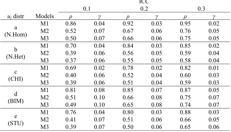
distributions and ICC values (0.1, 0.2, 0.3) with a fixed data structure (cs = 30 and nc = 100). Table 6 shows the results of the simulations in terms of both the Spearman correlation coefficient and γ= Pr(TE/NTT). As expected, in all scenarios, the higher the ICC, the better the
ranking: high values of the ICC indicate a strong school effect, and this facilitates the distinction among schools. In particular, the classification matrixes, here not reported for brevity, show that the positive effect of the ICC on ranking quality is spread over the entire distribution of uj. As found in the previous results, estimation model M1 performs better than
[image:18.612.113.500.493.714.2]the others in all situations.
Table 6. Spearman correlation coefficients (ρ) and Probability of misclassifying a Non-Top school as Top, γ = Pr(TE/NTT), for different estimation models, uj distributions and ICC values
uj distr Models
ICC
0.1 0.2 0.3
ρ γ ρ γ ρ γ
a (N.Hom)
M1 0.86 0.04 0.92 0.03 0.95 0.02
M2 0.52 0.07 0.67 0.06 0.76 0.05
M3 0.50 0.07 0.66 0.06 0.75 0.05
b (N.Het)
M1 0.70 0.04 0.84 0.03 0.85 0.02 M2 0.39 0.06 0.56 0.05 0.59 0.04 M3 0.37 0.06 0.55 0.05 0.58 0.04
c (CHI)
M1 0.69 0.02 0.78 0.02 0.82 0.01 M2 0.40 0.06 0.52 0.04 0.60 0.03
M3 0.39 0.06 0.51 0.04 0.59 0.03
d (BIM)
M1 0.81 0.08 0.85 0.07 0.87 0.05 M2 0.51 0.10 0.66 0.08 0.75 0.07 M3 0.49 0.10 0.65 0.08 0.74 0.07
e (STU)
In our final simulations we assess the role of the difference in the between and within effects of the covariates included in the model. Let the quantities 1 1W1Band
2 2
2 W B
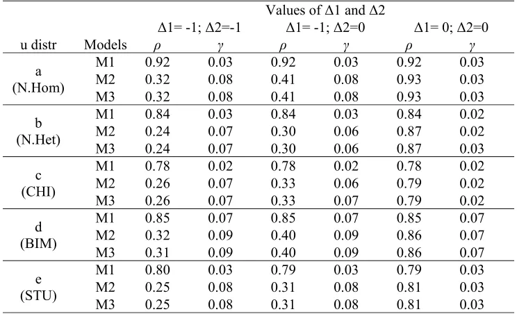
measure the difference in the within-between effects for the two covariates imposed in the data generating model. Given our discussion in section 2, we expect better performance of model M1 relative to model M2 and M3 for higher values of Δ1 and Δ2. In the simulations we vary the values of both Δ1and Δ2 in the set {-1; 0; +1}. Table 7 reports the results for three out of the nine possible combinations. The results not reported here, but available from the authors upon request, show that the situations characterised by the same absolute value of the sum of Δ1 and Δ2 are equivalent in terms of ranking quality. For example, the case
Δ1 = Δ2 = -1 is equivalent to the cases Δ1= -1 and Δ2 = +1; Δ1 = +1 and Δ2 = -1; and
Δ1 = Δ2 = +1. Therefore, what seems to matter is the overall absolute value of the
discrepancies in the between and within effects of the covariates and not the sign of the two differences.
From table 7 we see that, if for each covariate the within and between effects are equal (Δ1=0 and Δ2=0), the results from the three models are, as expected, almost indistinguishable, irrespective of the true second level error distribution. This is the case also for other values of the ICC, nc and cs (results of these simulations are not shown here but available upon
[image:19.612.120.492.386.612.2]request). On the contrary, the models become more different and the relative performance of model M1 increases when the number of covariates with a discrepancy in the between-within effects and/or the absolute value of the discrepancy is increased.
Table 7. Spearman correlation coefficients and γ= Pr(TE/NTT) for different values of the
difference W B
r r
r
(r=1,2) and uj distributions
u distr Models
Values of Δ1 and Δ2
Δ1= -1; Δ2=-1 Δ1= -1; Δ2=0 Δ1= 0; Δ2=0
ρ γ ρ γ ρ γ
a (N.Hom)
M1 0.92 0.03 0.92 0.03 0.92 0.03
M2 0.32 0.08 0.41 0.08 0.93 0.03
M3 0.32 0.08 0.41 0.08 0.93 0.03
b (N.Het)
M1 0.84 0.03 0.84 0.03 0.84 0.02
M2 0.24 0.07 0.30 0.06 0.87 0.02
M3 0.24 0.07 0.30 0.06 0.87 0.03
c (CHI)
M1 0.78 0.02 0.78 0.02 0.78 0.02
M2 0.26 0.07 0.33 0.06 0.79 0.02
M3 0.26 0.07 0.33 0.07 0.79 0.02
d (BIM)
M1 0.85 0.07 0.85 0.07 0.85 0.07
M2 0.32 0.09 0.40 0.09 0.86 0.07
M3 0.31 0.09 0.40 0.09 0.86 0.07
e (STU)
M1 0.80 0.03 0.79 0.03 0.79 0.03
M2 0.25 0.08 0.31 0.08 0.81 0.03
M3 0.25 0.08 0.31 0.08 0.81 0.03
5. Summary and discussion
We compared three models that can be used by practitioners in order to rank institutions: two multilevel models (with and without cluster average of first-level covariates) and a one-level fixed effect model with cluster-specific intercepts. Several conclusions can be drawn from our work.
First, ranking is reliable only for extreme institutions. Consistently with the multilevel literature (Goldstein and Healy, 1995), we find that it is easier to reliably rank the institutions with extreme performances but it is hard to precisely rank the institutions with average performances. However, we do not think this is a reason to abandon the approach because extremely “bad” and “good” performing institutions are usually the most interesting for researchers and policy makers.
Second, the effect of non-normal errors at the second level can also be detrimental to ranking of extreme institutions. In particular, a highly asymmetric distribution (e.g., Chi-square) of second-level residuals implies a good ranking quality only of one tail of the distribution and a rather poor quality of the other tail. A bi-modal distribution, on the contrary, produces a low ranking quality for both tails. This highlights the importance of testing for normality of the residuals distribution. If non-normality of residuals cannot be easily solved by, for example, transforming the outcome variable, other approaches such as non-parametric estimation of random effects could be worth exploring. With respect to the data structure, large sample sizes help to increase the ranking quality while the number and size of clusters, per se, play a less important role. We also find that a large ICC facilitates the ranking.
Third, the assessment of ranking quality depends on the research/policy goals. While the performance of multilevel models in identifying the true best-performing (Top) institutions can be unsatisfactory in specific conditions, the probability of classifying a true Non Top institution as a Top institution (error γ) is always very low for all the setups we used in our simulation study. On the other hand, the error probability δ (associated with misclassifying a true Top institution as Non Top) is sometimes too high.
Finally, discrepancies in the between and within effects of covariates is a crucial point for the quality of the ranking. In all experimental situations, the multilevel model with cluster means, which allows the between and within effects of the covariates to be different, performs much better than the others. Only when the between and within effects are equal for all the
covariates, do the three models perform very similarly. These results highlight the importance, also for cluster ranking, to take into account that within-cluster and between-cluster
relationships can be very different when dealing with multilevel data structures. These results are in line with similar remarks made in the multilevel literature, for example by Neuhaus and Kalbfleisch (1998) and Skrondal and Rabe-Hesketh (2004).
example, the accountability system aims at investing on the worst schools to improve their performance, then missing investments due to misclassifying extreme schools as non-extreme are more costly. The probability of these misclassifications is higher and a model -djusted ranking approach could not be satisfactory.
Further research is, however, needed to understand the consequences on the ranking quality of other forms of model misspecifications, such as those caused by endogeneity problems, which may arise in the presence of measurement error or omitted variables. Moreover, it would be interesting to consider unbalanced data structures and to extend the analysis to the non-linear case.
References
Aassve, A. & Arpino, B. (2007). Dynamic Multi-Level Analysis of Households' Living Standards and Poverty: Evidence from Vietnam. Working Paper of Institute for Social and Economic Research, paper 2007-10. Colchester: University of Essex.
Adab, P., Rouse. A., Mohammed, M.A., & Marshall. T. (2002). Performance league tables: the NHS deserves better. BMJ, 324, 95–98.
Aitkin, M., & Longford, N. (1986). Statistical modelling in school effectiveness studies (with discussion). Journal of Royal Statistical Society A, 149, 1-42.
Chiandotto, C. & Varriale, R. (2005). Un modello multilivello per l’analisi dei tempi di conseguimento del titolo nell’Ateneo fiorentino, in C. Crocetta (Ed.), Modelli di analisi della transizione università-lavoro. Vol.7, Cleup, Padova.
Downey, D.B., von Hippel, P.T., &Hughes, M. (2008). Are “failing” schools really failing? Using seasonal comparison to evaluate school effectiveness. Sociology of Education, 81(3), 242-270
Goldstein, H. & Healy, M.J.R. (1995). The graphical presentation of a collection of means.
Journal of the Royal Statistical Society, 158, 175-177.
Goldstein, H. & Spiegelhalter, D.J. (1996). League tables and their limitations: statistical issues in comparisons of institutional performance. Journal of the Royal Statistical Society: Series A, 159, 385-443.
Goldstein, H., Rasbash, J., Yang, M., Woodhouse, G., Pan, H., Nuttall, D., & Thomas, S. (1993). A multilevel analysis of school examination results. Oxford Review of Education, 19, 425-433.
Jürges, H, & Sneider, K. (2007). Fair ranking of teachers. Empirical Economics, 32, 411-431. Ladd, H. F., & Walsh, R.P. (2002). Implementing value-added measures of school
effectiveness: getting the incentives right. Economics of Education Review, 21, 1-17. Leckie, G. & Goldstein, H. (2009). The Limitations of Using School League Tables to Inform
School Choice. The Centre for Market and Public Organisation 09/208, Department of Economics, University of Bristol, UK.
Maas, C.J.M. and Hox. J.J. (2004). Robustness issues in multilevel regression analysis.
Statistica Neerlandica, 58(2), 127–137.
Maddala, G.S. (1971). The use of variance components models in pooling cross section and time series data. Econometrica, 39 (2), 341-358.
Neuhaus, J.M. & Kalbfleisch, J.D. (1998). Between- and within-cluster covariate effects in the analysis of clustered data. Biometrics, 54, 638-645.
Rampichini, C., Grilli, L., & Petrucci, A. (2004). Analysis of university course evaluations: from descriptive measures to multilevel models. Statistical Methods and Applications, 13(3), 357-373.
Raudenbush, S.W., & Willis, J.D. (1995). The estimation of school effects. Journal of Educational and Behavioral Statistics, 20, 307-335.
Shaw, C.D. & Costain, D.W. (1995). League tables for health care. Journal of the Royal Society of Medicine, 88, 54-57.
Skrondal, A. & Rabe-Hesketh, S. (2004). Generalized Latent Variable Modelling: Multilevel, Longitudinal and Structural Equation Models. Boca Raton, FL: Chapman & Hall/CRC. Snijders, T., & Bosker, R.(1999). An Introduction to Basic and Advanced MultileveModeling.
Sage, London.
Tekwe, C.D., Carter, R.L., Ma, C., Algina, J. Lucas, M.E., Roth, J. Ariet, M., Fisher, T., & Resnick, M.B. (2004). An empirical comparison of statistical models for value-added assessment of school performance. Journal of Educational and Behavioral Statistics, 29 (1), 11-35
Wößmann, L. (2008). Efficiency and equity of European education and training policies.