We Are Living in a Computer Simulation

http://dx.doi.org/10.4236/jmp.2016.710110

We Are Living in a Computer Simulation

Ding-Yu Chung

Utica, MI, USA

Received 10 May 2016; accepted 24 June 2016; published 28 June 2016

Copyright © 2016 by author and Scientific Research Publishing Inc.

This work is licensed under the Creative Commons Attribution International License (CC BY).

http://creativecommons.org/licenses/by/4.0/

Abstract

This paper posits that we are living in a computer simulation to simulate physical reality which has the same computer simulation process as virtual reality (computer-simulated reality). The computer simulation process involves the digital representation of data, the mathematical com-putation of the digitized data in geometric formation and transformation in space-time, and the selective retention of events in a narrative. Conventional physics cannot explain physical reality clearly, while computer-simulated physics can explain physical reality clearly by using the com-puter simulation process consisting of the digital representation component, the mathematical computation component, and the selective retention component. For the digital representation component, the three intrinsic data (properties) are rest mass-kinetic energy, electric charge, and spin which are represented by the digital space structure, the digital spin, and the digital electric charge, respectively. The digital representations of rest mass and kinetic energy are 1 as attach-ment space for the space of matter and 0 as detachattach-ment space for the zero-space of matter, re-spectively, to explain the Higgs field, the reverse Higgs field, quantum mechanics, special relativity, force fields, dark matter, and baryonic matter. The digital representations of the exclusive and the inclusive occupations of positions are 1/2 spin fermion and integer spin boson, respectively, to explain spatial translation by supersymmetry transformation and dark energy. The digital repre-sentations of the allowance and the disallowance of irreversible kinetic energy are integral elec-tric charges and fractional elecelec-tric charges, respectively, to explain the confinements of quarks and quasiparticles. For the mathematical computation component, the mathematical computation involves the reversible multiverse and oscillating M-theory as oscillating membrane-string-par- ticle whose space-time dimension (D) number oscillates between 11D and 10D and between 10D and 4D to explain cosmology. For the selective retention component, gravity, the strong force, electromagnetism, and the weak force are the retained events during the reversible four-stage evolution of our universe, and are unified by the common narrative of the evolution.

Keywords

Reverse Higgs Field, Fractional Electric Charge, Spin, Multiverse, Cosmology, Force Fields, Cyclic Universe

1. Introduction

In the simulation hypothesis by Nick Bostrom [1], physical reality is actually a computer simulation. We are living in a computer simulation which is derived from the mathematical computation based on the fundamental laws of physics. In the future, the computer will be powerful enough to compute all details in physical reality, and will create a computer-simulated world. Currently, it is possible to simulate virtual reality by digital com-puter. Virtual reality is digital computer-simulated reality. Virtual reality is used in flight simulation to train people to be pilots. The model of the typical digital computer is often called the von Neumann computer as Figure 1.

In a digital computer, input data from the input unit are converted into digitized data. For the computer simu-lation process for virtual reality, the computation section of the Central Process Unit (CPU) computes digitized data in geometric formation and transformation in space-time, while the control section of the CPU handles the logistics of digitized data. Selective digitized data are retained in memory. The computed digitized data are converted into data which appear as output data in the output unit. As a result, the computer simulation process for virtual reality involves the three components consisting of the digital representation component, the mathe-matical computation component, and the selective retention component. In the digital representation component, data are represented by digital representations. Both data and digital representations of data exist. The mathe-matical computation component computes digitized data in geometric formation and transformation in space- time. The selective retention component retains selectively events in a narrative. There is no logical relation among all retained events. The retained events are unified by the common narrative.

This paper posits that we are living in a computer simulation to simulate physical reality which has the same computer simulation process as virtual reality (computer-simulated reality). Both computer simulation processes for physical reality and virtual reality involve the digital representation of data, the mathematical computation of the digitized data in geometric formation and transformation in space-time, and the selective retention of events in a narrative. For the digital representation component of physical reality, the three intrinsic data (properties) are rest mass-kinetic energy, electric charge, and spin which are represented by the digital space structure [2]-[4], the digital spin, and the digital electric charge [5], respectively. As described previously for the digital space structure [2]-[4], the digital representations of rest mass and kinetic energy are 1 as attachment space for the space of matter and 0 as detachment space for the zero-space of matter, respectively. In the digital space struc-ture, attachment space attaches to matter permanently or reversibly. Detachment space detaches from the object at the speed of light. Attachment space relates to rest mass and reversible movement, while detachment space relates to irreversible kinetic energy. Attachment space and detachment space are the origins of the Higgs field and the reverse Higgs field, respectively. The combination of n units of attachment space as 1 and n units of de-tachment space as 0 brings about the three digital structures: binary partition space (1)n(0)n, miscible space (1 +

0)n, and binary lattice space (1 0)n to account for quantum mechanics, special relativity, and the force fields,

re-spectively. The digital representations of the exclusive and the inclusive occupations of positions are 1/2 spin fermion and integer spin boson, respectively. Fermions, such as electrons and protons, follow the Pauli exclu-sion principle which excludes fermions of the same quantum-mechanical state from being in the same position. Bosons, such as photons or helium atoms, follow the Bose-Einstein statistics which allows bosons of the same quantum-mechanical state being in the same position. The exclusion-inclusion brings about spatial translation by the supersymmetry transformations between fermion and boson. As described previously for the digital electric

charge [5], the digital repre-sentations of the allowance and the disallowance of irreversible kinetic energy are integral electric charges and fractional electric charges, respectively. Quarks in hadrons and quasiparticles in the Fractional Quantum Hall Effect (FQHE) have fractional electric charges whose irreversible movement caused by irreversible kinetic energy is restricted within hadrons and within the confinement of two-dimensional sys-tems, respectively.

For the mathematical computation of physical reality, the mathematical computation involves geometric for-mation and transforfor-mation in space-time, and as described before [3][4], physical reality involves oscillating M- theory instead of conventional fixed M-theory. In oscillating M-theory as oscillating membrane-string-particle, space-time dimension (D) number oscillates between 11D and 10D and between 10D and 4D. Space-time di-mension number between 10 and 4 decreases with decreasing speed of light, decreasing vacuum energy, and in-creasing rest mass.

The selective retention component for physical reality is narrative. For physical reality, the unification of the four force fields (gravity, the strong force, electromagnetism, and the weak force) based on a symmetry group has not been successful. There is no logical relation among the four force fields. In the computer simulation process for virtual reality, it is possible to retain events at different times in a narrative in such way that different events are unified by the common narrative. As described before [6]-[9], the four force fields in our universe are the retained events during the four-stage evolution of our universe, and are unified by the common narrative of the evolution.

Conventional physics cannot explain the reality of quantum mechanics easily. Conventional physics cannot explain the origins of the confinement of quarks and the fractional charges of quasiparticles. The geometry in conventional physics is fixed M-theory which has no experimental proof. Conventional physics cannot unify the four force fields. Conventional physics cannot explain physical reality clearly, while computer-simulated phys-ics can explain physical reality clearly [4][5] by using the computer simulation process consisting of the digital representation component, the mathematical computation component, and the selective retention component. We are living in a computer simulation.

Section 2 describes the mathematic computation component for oscillating M-theory. Section 3 explains the digital representation component consisting of the digital space structure, the digital spin, and the digital electric charge. Section 4 describes the narrative of the evolution of our universe to unify the four force fields.

2. The Mathematical Computation Component

The geometry in the mathematic computation component for the computer simulation process is oscillating M-theory. M-theory with eleven-dimensional membrane is an extension of string theory with ten-dimensional string, in contrast to the observed 4D. In conventional M-theory, space-time dimensional number (D) is fixed. As a result, the observed 4D results from the the compactization of the extra space dimensions in 11D M-theory, However, there is no experimental proof for compactized extra space dimensions, and there are numerous ways for the compactization of the extra space dimensions [10]. As described before [3][4], the geometry for the ma-thematical computation is oscillating M-theory derived from oscillating membrane-string-particle whose space-time dimension number oscillates between 11D and 10D and between 10D and 4D dimension by dimension reversibly. There is no compactization. Matters in oscillating M-theory include 11D membrane (211) as membrane (denoted

as 2 for 2 space dimensions) in 11D, 10D string (110) as string (denoted as 1 for 1 space dimension) in 10D, and

variable D particle (04 to 11) as particle (denoted as 0 for 0 space dimension) in 4D to 11D.

As described previously [3] [4], the QVSL (quantum varying speed of light) transformation transforms both space-time dimension number (D) and mass dimension number (d). In the QVSL transformation, the decrease in the speed of light leads to the decrease in space-time dimension number and the increase of mass in terms of increasing mass dimension number from 4 to 10,

D 4

D ,

c =c α − (1a) ( )

(

2 2 D 4

)

0

E=M ⋅ c α − (1b) ( )

(

2 d 4

)

2

0 .

M α − c

= ⋅ (1c)

2

D D ,

n n

2 0,D,d 0,D ,d ,

n n n

M =M _{− +}

α

(1e)

(

) (

)

QVSL

D, d→ Dn , d±n (1f)

2 vacuum,D 0,D ,

E = −E M c (1g) where cD is the quantized varying speed of light in space-time dimension number, D, from 4 to 10, c is the observed

speed of light in the 4D space-time, α is the fine structure constant for electromagnetism, E is energy, M0 is rest mass,

D is the space-time dimension number from 4 to 10, d is the mass dimension number from 4 to 10, n is an integer, and Evacuum = vacuum energy. For example, in the QVSL transformation, a particle with 10D4d is transformed to a

particle with 4D10d from Equation (1f). Calculated from Equation (1e), the rest mass of 4D10d is 1/α12≈ 13712 times of the mass of 10D4d. In terms of rest mass, 10D space-time has 4d with the lowest rest mass, and 4D space-time has 10d with the highest rest mass. Rest mass decreases with increasing space-time dimension number. The decrease in rest mass means the increase in vacuum energy (Evacuum,D), so vacuum energy increases with

in-creasing space-time dimension number. The vacuum energy of 4D particle is zero from Equation (1g). The mass dimension number is limited from 4 to 10, because 4D is the minimum space-time, and 11D membrane and 10D string are equal in the speed of light, rest mass, and vacuum energy. Since the speed of light for > 4D particle is greater than the speed of light for 4D particle, the observation of > 4D superluminal particles by 4D particles vi-olates casualty. Thus, > 4D particles are hidden particles with respect to 4D particles. Particles with different space-time dimensions are transparent and oblivious to one another, and separate from one another if possible.

As described previously [3] [4], another part of the mathematical computation component is the reversible multiverse. In the reversible multiverse, all physical laws and phenomena are permanently reversible, and tem-porary irreversibility of entropy increase is allowed through reversibility breaking, symmetry violation, and low entropy beginning. We live in the universe with such temporary irreversible entropy increase. The reversible universe is shown in cosmology which is in Section 4.

3. The Digital Representation Component

In the digital representation component for the computer simulation process, data in physical reality are represented by digital representations. Both data and digital representations exist. In physical reality, the three intrinsic data (properties) are rest mass-kinetic energy, spin, and electric charge which have the three digital re-presentations consisting of the digital space structure, the digital spin, and the digital electric charge for the in-trinsic data (properties) of rest mass-kinetic energy, spin, and electric charge, respectively.

3.1. Digital Space Structure

The digital representations of rest mass and kinetic energy are 1 as attachment space for the space of matter and 0 as detachment space for the zero-space of matter, respectively. In the digital space structure, attachment space attaches to matter permanently or reversibly. Detachment space detaches from the object at the speed of light. Attachment space relates to rest mass and reversible movement, while detachment space relates to irreversible kinetic energy.

In conventional physics, space does not couple with particles. In the Higgs field, space is the passive ze-ro-energy ground state space. Under spontaneous symmetry breaking, the passive zeze-ro-energy ground state is converted into the active, permanent, and ubiquitous nonzero-energy Higgs field, which couples with massless particle to produce the transitional Higgs field-particle composite. Under spontaneous symmetry restoring, the transitional Higgs field-particle composite is converted into the massive particle with the longitudinal component on zero-energy ground state without the Higgs field as follows.

[

]

spontaneous symmetry breaking

massless particle

spontaneous symmetry restorin

zerro-energy groud state space nonzero-energy scalar Higgs field

the transitional nonzero- energy Higgs field-particle composite

→

→

g _{massive particle with the longitudinal component}

on zero-energy ground state space without the Higgs field

→ (2)

with such nonzero-energy field is the cosmological constant problem from the huge gravitational effect by the nonzero-energy Higgs field in contrast to the observation [11].

As described before [4], in the digital space structure, space as the zero-energy ground state space couples with particles, unlike passive space in conventional physics. Attachment space is the origin of the Higgs field. Under spontaneous symmetry breaking, attachment space as the active zero-energy ground state space couples with massless particle to form momentarily the transitional non-zero energy Higgs field-particle composite. The Higgs field is momentary and transitional, avoiding the cosmological constant problem. Under spontaneous symmetry restoring, the transitional nonzero-energy Higgs field-particle composite is converted into massive particle with the longitudinal component on zero-energy attachment space without the Higgs field as follows.

[

]

spontaneous symmetry breaking

spontaneous symmetry restoring

massless particle zero-energy attachment space

the transitional non-zero energy Higgs field-particle composite

massive particle with the lon

+ →

→ gitudinal

component on zero-energy attachment space without the Higgs field

(3)

Detachment space is the origin of the reverse Higgs field. Unlike the conventional model, detachment space actively couples to massive particle. Under spontaneous symmetry breaking, the coupling of massive particle to zero-energy detachment space produces the transitional nonzero-energy reverse Higgs field-particle composite which under spontaneous symmetry restoring produces massless particle on zero-energy detachment space without the longitudinal component without the reverse Higgs field as follows.

[

]

spontaneous symmetry breaking

spontaneous symmetry restoring

massive particle zero-energy detachment space

the transitional nonzero-energy reverse Higgs field-particle composite

massless particle wit

+ →

→ hout the longitudinal

component on zero-energy detachment space without the reverse Higgs field

(4)

For the electroweak interaction in the Standard model where the electromagnetic interaction and the weak in-teraction are combined into one symmetry group, under spontaneous symmetry breaking, the coupling of the massless weak W, weak Z, and electromagnetic A (photon) bosons to zero-energy attachment space produces the transitional nonzero-energy Higgs fields-bosons composites which under partial spontaneous symmetry res-toring produce massive W and Z bosons on zero-energy attachment space with the longitudinal component without the Higgs field, massless A (photon), and massive Higgs boson as follows.

[

]

spontaneous symmetry breaking

massless WZ zero-energy WZ attachment space massless A zero-energy A attachment space A

the transitional nonzero-energy WZ Higgs field -WZ composite

nonzero-energy A Higgs field -A comp

+ + +

→

+

[

]

partial spontaneous symmetry restoring

osite

massive WZ with the longitudinal component on attachment space without the Higgs field

massless A the nonzero energy massive Higgs boson

→

+ +

(5)

From the periodic table of elementary particles, the theoretical calculated mass of the Higgs boson is 128.8 GeV in good agreements with the observed 125 or 126 GeV [12]. In terms of mathematical expression, the con-ventional permanent Higgs field model and the posited transitional Higgs field model are identical. The inter-pretations of the mathematical expression are different for the permanent Higgs field model and the transitional Higgs field model. The transitional Higgs field model avoids the cosmological problem in the permanent Higgs field model.

As shown in Section 4, our universe is the dual asymmetrical positive-energy-negative-energy universe where the positive-energy universe on attachment space absorbed the interuniversal void on detachment space to result in the combination of attachment space and detachment space, and the negative-energy universe did not absorb the interu-niversal void. The combination of n units of attachment space as 1 and n units of detachment space as 0 brings about three different digital space structures: binary partition space, miscible space, or binary lattice space as below.

( )

( )

combination

( ) ( )

(

)

( )

1 0 1 0 , 1 0 , or 1 0

attachment space , detachment space , binary partition space , miscible space , binary lattice space

Binary partition space, (1)n(0)n, consists of two separated continuous phases of multiple quantized units of

at-tachment space and deat-tachment space. In miscible space, (1 + 0)n, attachment space is miscible to detachment

space, and there is no separation of attachment space and detachment space. Binary lattice space, (1 0)n, consists

of repetitive units of alternative attachment space and detachment space. In conventional physics, space does not couple with particles, and does not contain detailed structure. In the digital space structure, space couples with particles, and contains the three different digital structures.

Binary partition space (1)n(0)n can be described by the uncertainty principle. The uncertainty principle for

quantum mechanics is expressed as follows.

2

x p

σ σ ≥ (7)

The position, x, and momentum, p, of a particle cannot be simultaneously measured with arbitrarily high pre-cision. The uncertainty principle requires every physical system to have a zero-point energy (non-zero minimum momentum) and to have a non-zero minimum wavelength as the Planck length. In terms of the space structure, detachment space relating to kinetic energy as momentum is σp, and attachment space relating to space (wave-length) for a particle is σx. In binary partition space, neither detachment space nor attachment space is zero in the uncertainty principle, and detachment space is inversely proportional to attachment space. Quantum mechanics for a particle follows the uncertainty principle defined by binary partition space. Binary partition space (1)n(0)n

can also be described by the Schrodinger in quantum mechanics where total energy equals to kinetic energy re-lated to (0)n plus potential energy related to (1)n. In binary partition space, an entity is both in constant motion as

standing wave for detachment space and in stationary state as a particle for attachment space, resulting in the wave-particle duality.

Detachment space contains no matter that transmits information. Without transmitting information, detach-ment space is outside of the realm of causality. Without causality, distance (space) and time do not matter to de-tachment space, resulting in non-localizable and non-countable space-time. The requirement for the system (bi-nary lattice space) containing non-localizable and non-countable detachment space is the absence of net infor-mation by any change in the space-time of detachment space. All changes have to be coordinated to result in zero net information. This coordinated non-localized binary lattice space corresponds to nilpotent space. All changes in energy, momentum, mass, time, space have to result in zero [13]. The non-local property of binary lattice space for wave function provides the violation of Bell inequalities [14] in quantum mechanics in terms of faster-than-light influence and indefinite property before measurement. The non-locality in Bell inequalities does not result in net new information. Binary partition space explains the nonlocal pilot-wave theory (Bohmian mechanics) where the trajectories of particles are nonlocal and fully determined by the pilot wave [15].

In binary partition space, for every detachment space, there is its corresponding adjacent attachment space. Thus, no part of the mass-energy can be irreversibly separated from binary partition space, and no part of a dif-ferent mass-energy can be incorporated in binary partition space. Binary partition space represents coherence as wavefunction. Binary partition space is for coherent system. Any destruction of the coherence by the addition of a different mass-energy to the mass-energy causes the collapse of binary partition space into miscible space. The collapse is a phase transition from binary partition space to miscible space.

( ) ( )

collapse

(

)

0 1 0 1

binary partition space miscible space n

n n → + ₍₈₎

Another way to convert binary partition space into miscible space is gravity. Penrose [16] pointed out that the gravity of a small object is not strong enough to pull different states into one location. On the other hand, the gravity of large object pulls different quantum states into one location to become miscible space. Therefore, a small object without outside interference is always in binary partition space, while a large object is never in bi-nary partition space.

HΨ = ΨE (9) In miscible space, attachment space is miscible to detachment space, and there is no separation of attachment space and detachment space. In miscible space, attachment space contributes zero speed, while detachment space contributes the speed of light. For a moving massive particle consisting of a rest massive part and a massless part, the massive part with rest mass, m0, is in attachment space, and the massless part with kinetic energy, K, is adjacent to

detachment space. The combination of the massive part in attachment space and massless part in detachment leads to the propagation speed in between zero and the speed of light. To maintain the speed of light constant for a moving particle, the time (t) in moving particle has to be dilated, and the length (L) has to be contracted relative to the rest frame.

2 2

0 0

0

2 2

0 0

1 ,

,

t t c t L L

E K m c m c

υ γ

γ γ

= − =

=

= + =

(10)

where γ _{=1 1}

(

_{−v c}2 2

)

1 2 _{is the Lorentz factor for time dilation, and length contraction, E is the total energy, and}

K is the kinetic energy.

Bounias and Krasnoholovets [17] propose that the reduction of dimension can be done by slicing dimension, such as slicing 3 space dimension object (block) into infinite units of 2 space dimension objects (sheets). As shown in Section 4, the positive-energy 10D4d particle universe as our observable universe with high vacuum energy was transformed into the 4D10d universe with zero vacuum energy at once, resulting in the inflation. During the Big Bang following the inflation, the 10d (mass dimension) particle in attachment space denoted as 1 was sliced by de-tachment space denoted as 0. For example, the slicing of 10d particle into 4d particle is as follows.

(

)

10 slicing

10 4 4 4 ,d

d 5

1 1 0 1

10d particle 4d core particle binary lattice space

n

=

→

∑

(11)

where 110 is 10d particle, 14 is 4d particle, d is the mass dimension number of the dimension to be sliced, n as the

number of slices for each dimension, and (04 14)n is binary lattice space with repetitive units of alternative 4d

at-tachment space and 4d deat-tachment space. For 4d particle starting from 10d particle, the mass dimension number of the dimension to be sliced is from d = 5 to d = 10. Each mass dimension is sliced into infinite quantized units (n = ∞) of binary lattice space, (04 14)∞. For 4d particle, the 4d core particle is surrounded by 6 types (from d = 5

to d = 10) of infinite quantized units of binary lattice space. Such infinite quantized units of binary lattice space represent the infinite units (n = ∞) of separate virtual orbitals in a gauge force field, while the dimension to be sliced is “dimensional orbital” (DO), representing a type of gauge force field. The mass-energy in each dimen-sional orbital increases with the number of dimension number, and the lowest dimension orbital with d = 5 has the lowest mass-energy [9][18]. 10d particle was sliced into six different particles: 9d, 8d, 7d, 6d, 5d, and 4d equally by mass. Baryonic matter is 4d, while dark matter consists of the other five types of particles (9d, 8d, 7d, 6d, and 5d).

(

)

(

)

the inflation the Big Bang

10D4d 4D10d

baryonic matter( 4D4d dark matter 4D5d, 4D6d, 4D7d, 4D8d, 4D9d kinetic energy

→ →

+ + (12)

The mass ratio of dark matter to baryonic matter is 5 to 1. At 72.8% dark energy, the calculated values for baryonic matter and dark matter (with the 1:5 ratio) are 4.53% (= (100 – 72.8)/6) and 22.7% (= 4.53 × 5), re-spectively, in excellent agreement with observed 4.56% and 22.7%, respectively [9][19][20]. The dimensional orbitals of baryonic matter provide the base for the periodic table of elementary particles to calculate accurately the masses of all elementary particles, including quarks, leptons, gauge bosons, the Higgs boson, and the knees-ankles-toe in cosmic rays [12] [18][21]. The calculated masses of all elementary particles are in good agreement with the observed values. For examples, the calculated mass of top quark and the Higgs boson are 176.5 GeV and 128.8 GeV in good agreement with the observed 173.34 GeV and 125 or 126 GeV, respectively.

orbit-als) is the only one with the lowest dimensional orbital for electromagnetism. With higher dimensional orbitals, dark matter does not have this lowest dimensional orbital [6][18]. Without electromagnetism, dark matter cannot emit light, and is incompatible to baryonic matter with electromagnetism, like the incompatibility between oil and water. Derived from the incompatibility between dark matter and baryonic matter, the modified interfacial gravity (MIG) between homogeneous baryonic matter region and homogeneous dark matter region to separate baryonic matter region and dark matter region explains galaxy evolution and unifies the CDM (Cold Dark Matter) model, MOG (Modified Gravity), and MOND (Modified Newtonian Dynamics) [22][23]. The digital space structure based on the combination of binary partition space and binary lattice space explains superconductivity [24] and superstar without singularity to replace black hole with singularity [25][26]. Singularity is permanently irreversible by losing information permanently, forbidden in the reversible multiverse.

3.2. The Digital Spin

The digital representations of the exclusive and the inclusive occupations of positions are 1/2 spin fermion and integer spin boson, respectively. Fermions, such as electrons and protons, follow the Pauli exclusion principle which excludes fermions of the same quantum-mechanical state from being in the same position. Bosons, such as photons or helium atoms, follow the Bose-Einstein statistics which allows bosons of the same quantum-me- chanical state being in the same position. As a result, the digital representations of the exclusive and the inclusive occupations of positions are 1/2 spin fermion and integer spin boson, respectively. The symmetry between fer-mion and boson is supersymmetry. Two supersymmetry transformations from boson to ferfer-mion and from ferfer-mion to boson yield a spatial translation. In physical reality, supersymmetry is varying supersymmetry [3][4]. In va-rying supersymmetry, the repetitive transformation between fermion and boson brings about a spatial translation and the transformation into the adjacent mass dimension number. Varying supersymmetry transformation is one of the two steps in transformation involving the oscillation between 10D particle and 4D particle. The transfor-mation during the oscillation between 10D particle and 4D particle involves the stepwise two-step transfortransfor-mation consisting of the QVSL transformation and the varying supersymmetry transformation. As described in Section 2, the QVSL transformation involves the transformation of space-time dimension, D whose mass increases with decreasing D for the decrease in vacuum energy. The varying supersymmetry transformation involves the trans-formation of the mass dimension number, d whose mass decreases with decreasing d for the fractionalization of particle, as follows.

(

) (

)

(

)

QVSL

varying supersymmetry

stepwise two-step varying transformation

(1) D, d D 1 , d 1

(2) D, d D, d 1

←→ ±

←→ ±

 (13)

The repetitive stepwise two-step transformation between 10D4d and 4D4d as follows.

10D4d↔9D5d↔9D4d↔8D5d↔↔4D5d↔4D4d (14) In this two-step transformation, the transformation from 10D4d to 9D5d involves the QVSL transformation as in Equation (1d). Calculated from Equation (1e), the mass of 9D5d is 1/α2≈ 1372 times of the mass of 10D4d. The transformation of 9D5d to 9D4d involves the varying supersymmetry transformation. In the normal super-symmetry transformation, the repeated application of the fermion-boson supersuper-symmetry transformation carries over a boson (or fermion) from one point to the same boson (or fermion) at another point at the same mass. In the varying supersymmetry transformation, the repeated application of the fermion-boson supersymmetry trans-formation carries over a boson from one point to the boson at another point at different mass dimension number in the same space-time number. The repeated varying supersymmetry transformation carries over a boson Bd into a

fermion Fd and a fermion Fd to a boson Bd−1, which can be expressed as follows

d,F d,B d,B,

M =M

α

(15a)

d 1,B d,F d,F,

M − =M

α

(15b)

where Md, B and Md,F are the masses for a boson and a fermion, respectively, d is the mass dimension number, and

αd,B or αd,F is the fine structure constant that is the ratio between the masses of a boson and its fermionic partner.

2 d,B d 1,B d 1

M =M ₊

α

₊ . (15c) The mass of 9D4d is α2≈ (1/137)2 times of the mass of 9D5d through the varying supersymmetry transforma-tion. The transformation from a higher mass dimensional particle to the adjacent lower mass dimensional particle is the fractionalization of the higher dimensional particle to the many lower dimensional particles in such way that the number of lower dimensional particles becomes

( )

2 2

d 1 d d 137

N ₋ =N α ≈N (15d) The fractionalization also applies to D for 10D4d to 9D4d, so

2 D 1 D

N − =N α (15e)

Since the supersymmetry transformation involves translation, this stepwise varying supersymmetry transfor-mation leads to a translational fractionalization, resulting in the cosmic expansion. Afterward, the QVSL trans-formation transforms 9D4d into 8D5d with a higher mass. The two-step transtrans-formation repeats until 4D4d, and then reverses stepwise back to 10D4d for the cosmic contraction. The oscillation between 10D and 4D results in the reversible cyclic fractionalization-contraction for the reversible cyclic expansion-contraction of the universe which does not involve irreversible kinetic energy.

3.3. The Digital Electric Charge

As described before [5], the digital representations of the allowance and the disallowance of irreversible kinetic energy are integral electric charges and fractional electric charges, respectively. Individual integral charge with irreversible kinetic energy to cause irreversible movement is allowed, while individual fractional charge with ir-reversible kinetic energy is disallowed. The disallowance of irir-reversible kinetic energy for individual fractional charge brings about the confinement of individual fractional charges to restrict the irreversible movement re-sulted from kinetic energy. Collective fractional charges are confined by the short-distance confinement force field where the sum of the collective fractional charges is integer. As a result, fractional charges are confined and collective. The confinement force field includes gluons in QCD (quantum chromodynamics) for collective fractional charge quarks in hadrons and the magnetic flux quanta for collective fractional charge quasiparticles in the fractional quantum Hall effect (FQHE) [27]-[29].

The collectivity of fractional charges requires the attachment of energy as flux quanta to bind fractional charges. As a result, the integer-fraction transformation from integral charges to fractional charges involves the integer-fraction transformation to incorporate flux quanta similar to the composite fermion theory for the FQHE [30][31]. There are two steps in the composite fermion theory for the FQHE. The first step is the formation of composite fermion by the attachment of an even number of magnetic flux quanta to electron. Composite fer-mions in the Landau levels are the “true particles” to produce the FQHE, while electrons in the Landau level are the true particles to produce the integral quantum Hall effect (IQHE). The IQHE is a manifestation of the Lan-dau level quantization of the electron kinetic energy. The second step is the conversion of integral charges to fractional charges in the collective mode of composite fermions. The IQHE in the collective mode of composite fermions is the FQHE as expressed by the filling factors υ’s related to electric charges.

even numbers of magnetic flux quanta

*

*

*

the composite fermion theory the first step :

electrons composite fermions

the second step for the collective mode of composite fermions :

for the IQHE

for the FQHE

2 1

2 1

m

m mn n

ν ν ν

ν

→

=

= =

± ±

* 1

for 1, for the Laughlin wavefunction of the FQHE 2n 1

ν = ν = +

(16)

respective-ly in the Landau levels. The composite fermion theory is used to compute preciserespective-ly a number of measurable quantities, such as the excitation gaps and exciton dispersions, the phase diagram of composite fermions with spin, the composite fermion mass, etc.

The integer-fraction transformation from integral charges to fractional charges consists of the three steps: 1) the attachment of an even number of flux quanta to individual integral charge fermions to form individual integral charge composite fermions, 2) the attachment of an odd number of flux quanta to individual integral charge composite fermions to form transitional collective integral charge composite bosons, and 3) the conver-sion of flux quanta into the confinement force field to confine collective fractional charge composite fermions converted from composite bosons. The first step of the integer-fraction transformation from integral charge to fractional charge is same as the first step in the composite fermion theory. The first step is the attachment of an even number of flux quanta to individual integral charge fermions to form individual integral charge composite fermions [28]. Flux quanta are the elementary units which interact with a system of integral charge fermions. The attachment of flux quanta to the fermions transforms them to composite particles. The attached flux quanta change the character of the composite particles from fermions to bosons and back to fermions. Composite par-ticles can be either fermions or bosons, depending on the number of attached flux quanta. A fermion with an even number of flux quanta becomes a composite fermion, while a fermion with an odd number of flux quanta becomes a composite boson. Fermions, such as electrons and protons, follow the Pauli exclusion principle which excludes fermions of the same quantum-mechanical state from being in the same position. Bosons, such as pho-tons or helium atoms, follow the Bose-Einstein statistics which allows bosons of the same quantum-mechanical state being in the same position. As a result, fermions are individualistic, while bosons are collectivistic. Com-posite fermions are individualistic, while comCom-posite bosons are collectivistic. In the first step, the attachment of an even number of flux quanta to each integral charge fermion provides these fermions individual integral charge composite fermions which follow the Pauli exclusion principle.

The second step involves the traditional composite bosons. The second step explains the origin of 1/(2n + 1) in Equation (16) in the second step of the composite fermion theory which does not explain the origin of 1/(2n + 1). The second step is the attachment of an odd number of flux quanta to individual integral charge composite fermions to form transitional collective integral charge composite bosons [28]. Individual integral charge com-posite fermions with an odd number (2n + 1) of flux quanta provide collective integral charge comcom-posite bosons which allow bosons of the same quantum-mechanical state being in the same position. The collective integral charge composite bosons allow the connection of collective flux quanta from collective integral charge compo-site bosons. Each flux quantum represents an energy level. In individual integral charge compocompo-sited fermions, the degenerate energy levels are separated. In collective integral charge composite bosons, the 2n +1 degenerate energy levels are connected into 2n + 1 sites in the same energy level.

The third step is the conversion of collective flux quanta into the confinement force field to confine collective fractional charge composite fermions converted from the collective integral charge composite bosons. In collec-tive fractional charge fermions, each site in the same energy level has ±1/(2n + 1) fractional charge.

1 fractional charge per site in the same energy level

2n 1 ± =

+ (17) Fractional charges are the integer multiples of ±1/(2n + 1) fractional charge to explain the origin of 1/(2n +1) in Equation (16) for the composite fermion theory. The products in the third step also include individual integral charge fermions to conserve electric charge. The sum of all collective fractional charges and individual integral charges is integer. The integer-fraction transformation from individual integral charge fermions to collective fractional charge fermions is as follows.

even number of flux quanta

odd number of flux quanta

confinement force field

individual IC fermions individual IC composite fermions

tramsitional collective IC composite bosons

collective FC compos

→

→

→ ite fermions+individual IC fermions

(18)

4. The Selective Retention Component

The selective retention component retains selectively events in a narrative. The retained events are unified by the common narrative. The narrative of physical reality is the four-stage evolution of our cyclic dual universe. The four force fields are unified by the four-stage evolution. For the narrative of our universe, our universe is in the reversible multiverse where all physical laws and phenomena are permanently reversible, and temporary irrever-sibility of entropy increase is allowed through reverirrever-sibility breaking, symmetry violation, and low entropy be-ginning. The multiverse has been studied extensively. For example, Brian Greene [32] described the nine types of the multiverse which produce complicated collections of universes. The reversible multiverse model is a sim-ple and neat version of the multiverse to exclude all permanently irreversible phenomena and physical laws. One irreversible phenomenon which is not allowed is the collision of expanding universes. The collision of expand-ing universes which have the inexhaustible resource of space-time to expand is permanently irreversible due to the impossibility to reverse the collision of expanding universes. To prevent the collision of expanding universes, every universe is surrounded by the interuniversal void that is functioned as the permanent gap among universes. The space in the interuniversal void is detachment space [6] which detaches matter and relates to kinetic energy. The interuniversal void has zero-energy, zero space-time, and zero vacuum energy, and detachment space only, while universe has nonzero-energy, the inexhaustible resource of space-time to expand, zero or/and non-zero vacuum energy, and attachment space with or without detachment space. Attachment space attaches matter and relates to rest mass. The detachment space of the interuniversal void has no space-time, so it cannot couple to particles with space-time in universes, but it prevents the advance of expanding universes to the interuniversal void to avoid the collision of expanding universes.

A zero-sum energy dual universe of positive-energy universe and negative-energy universe can be created in the zero-energy interuniversal void, and the new dual universe is again surrounded by the interuniversal void to avoid the collision of universes. Under symmetry, the new positive-energy universe and the new nega-tive-energy universe undergo mutual annihilation to reverse to the interuniversal void immediately. Our universe is the dual asymmetrical positive-energy-negative-energy universe where the positive-energy universe on at-tachment space absorbed the interuniversal void on deat-tachment space to result in the combination of atat-tachment space and detachment space, and the negative-energy universe did not absorb the interuniversal void. Within the positive-energy universe, the absorbed detachment space with space-time can couple to particles in the posi-tive-energy universe to result in massless particles with irreversible kinetic energy. The formation of our un-iverse involves symmetry violation between the positive-energy unun-iverse and the negative energy unun-iverse. Ir-reversible kinetic energy from detachment space is the source of irIr-reversible entropy increase, so the posi-tive-energy universe is locally irreversible, while the negaposi-tive-energy universe without irreversible kinetic energy from detachment space is locally reversible. The locally reversible negative-energy universe guides the reversible process of the dual universe. As a result, our whole dual universe is globally reversible. Our dual un-iverse is the globally reversible cyclic dual unun-iverse as shown in Figure 2 for the evolution of our unun-iverse as described previously [6]-[9].

The four reversible stages in the globally reversible cyclic dual universe are 1) the formation of the 11D membrane dual universe, 2) the formation of the 10D string dual universe, 3) the formation of the 10D particle dual universe, and 4) the formation of the asymmetrical dual universe.

1) The formation of the 11D membrane dual universe

As described previously [6]-[9], the reversible cyclic universe starts in the zero-energy interuniversal void, which produces the dual universe of the positive-energy 11D membrane universe and the negative-energy 11D mem-brane universe as in Figure 2. In some dual 11D memmem-brane universes, the 11D positive-energy memmem-brane un-iverse and the negative-energy 11D membrane unun-iverse coalesce to undergo annihilation and to return to the in-teruniversal void as in Figure 2.

2) The formation of the 10D string dual universe

Under the reversible oscillation between 11D and 10D, the positive-energy11D membrane universe and the negative-energy 11D membrane universe are transformed into the positive-energy 10D string universe and the negative-energy 10D string universe, respectively, as in Figure 2. The positive-energy 11D membrane universe is transformed into the positive-energy 10D string universe as in Equations (19a) and (19b).

( )

from11D membrane to 10D string

11 10

the close string vibration

10 10 10 10

The RS1 Membrane Transformation

step1: 2 1 in the 11D AdSspace

step 2 : 2 1 1 0 1 g_e in the 11D AdS space

→

→ =

[image:12.595.143.491.86.311.2]

Figure 2. The globally reversible cyclic dual universe.

( )

the close string and the open string vibrations

( )

11 10

2 2 ←→ s1 ge (19b) where 211 is membrane (denoted as 2) in 11D, s is the pre-strong force, 110 is string (denoted as 1) in 10D, 010is

particle (denoted as 0) in 10D, AdS is anti-de Sitter, and ge is the external graviton.

According Randall and Sundrum, the RS1 (Randall-Sundrum model 1) in an anti-de Sitter (AdS) space con-sists of one brane with extremely low graviton’s probability function and another brane with extreme high gra-viton’s probability function [33] [34]. The formation of the 10D string dual universe involves the RS1. As shown in Equation (19a), one of the possible membrane transformations from the 11D membrane to the 10D string is the RS1 membrane transformation which involves two steps. In the Step 1, the extra spatial dimension of the 11D membrane in the transformation from the 11D membrane to the 10D string becomes the spatial di-mension transverse to the string brane in the bulk 11D anti-de Sitter space [33]. This transformation is derived from the transformation from membrane to string. In the transformation from the two-dimensional membrane to the one-dimensional string, the extra spatial dimension of the two-dimensional membrane on the x-y plane be-comes the x-axis transverse to the one-dimensional string on the y-axis in the two-dimensional x-y space. In the Step 2, for the RS1 membrane transformation, two string branes are combined into the combined string brane. The external 10D particles generated by the close string vibration of the combined string brane are the 10D ex-ternal gravitons which form the exex-ternal graviton brane as the Gravitybrane (Planck Plane) in the RS1 of the Randall-Sundrum model [33] [34]. As in the RS1 of the Randall-Sundrum model, the two branes with equal mass- energy in the 11D anti-de Sitter space are the string brane with weak gravity and the external graviton brane with strong gravity. The weak gravity in the string brane is the predecessor of the observed weak gravity generated during the Big Bang [6][17]. The external graviton in the external graviton brane is the predecessor of a part of the observed dark energy [3][4]. The 10D string brane and the 10D external graviton brane correspond to the predecessors of the observed universe (without dark energy) and a part of observed dark energy, respec-tively [6][17]. The reverse transformation from 10D to 11D is the RS1 string transformation.

so the strong force becomes the confinement force for fractionally charge quarks which do not allow irreversible kinetic energy [5].

In the negative universe through symmetry, the 11D anti-membrane (2₋₁₁) is transformed into 10D antistring (1₋₁₀) with external anti-graviton g_e and the pre-strong force s as follows.

(

11

)

(

10

)

2 2− ←→ s1− ge (20) The dual universe of the positive-energy 10D string universe with n units of (110)n and the negative-energy 10D

string universe with n units of (1₋₁₀)n is as follows.

(

)

(

110 e

)

_n

(

e

(

110

)

)

n

s g g s ₋ (21) There are four equal regions: the positive-energy 10D string universe, the external graviton, the external an-ti-graviton, and the negative-energy 10D string universe.

Some dual 10D string universes return to the dual 11D membrane universes under the reversible oscillation between 11D and 10D. Alternatively, under symmetry violation as in the case of our universe, the positive-energy 10D string universe absorbs the interuniversal void, while the negative-energy 10D string universe does not ab-sorb the interuniversal void. The interuniversal void has zero vacuum energy. In our universe, the absorption of the interuniversal void by the positive-energy 10D string universe forced the positive-energy 10D universe with high vacuum energy to be transformed into the universe with zero vacuum energy that was the vacuum energy of the 4D universe. However, the transformation from 10D to 4D was not immediate, because the strings had to be 10D, and it could not be transformed into 4D, therefore, strings had to be transformed into particles that allowed the change of its dimension number freely to accommodate the transformation from the 10D universe to the 4D universe driven by the absorption of the interuniversal void.

3) The formation of the 10D particle dual universe

As described previously [9][17], the transformation of strings into particles came from the emergence of posi-tive charge and negaposi-tive charge that allowed the mutual annihilation of posiposi-tively charged 10D strings and tively charged 10D antistrings in the 10D string universes to produce positively charged 10D particles and nega-tively pre-charged 10D antiparticles in the 10D particle universes as follows.

(

)

(

010 010 e

)

(

e

(

010 010

)

)

,

n n

s e e+ − − s g g s e e+ − − s (22)

where s and e are the pre-strong force and the pre-charged force in the flat space, ge is the external graviton, ge is the external graviton, and 0100−10 is the particle-antiparticle. There are four equal regions: the 10D

posi-tive-energy particle universe, the external graviton, the 10D negaposi-tive-energy particle universe, and the external anti-graviton. The emergence of positive charge and negative charge provides the prototype of the observed elec-tromagnetic force with charge generated during the Big Bang [6][17].

4) The formation of the asymmetrical dual universe

The formation of our current universe follows immediately after the formation of the 10D particle dual un-iverse through the asymmetrical dimensional oscillations, leading to the asymmetrical dual unun-iverse. The 10D positive-energy universe was transformed immediately into the 4D positive-energy particle universe with zero vacuum energy. The 10D negative-energy particle universe undergoes the stepwise dimension number oscilla-tion between 10D and 4D. Without absorbing the interuniversal void, the external graviton and the anti-graviton also undergo the stepwise dimension number oscillation between 10D and 4D. The result is the asymmetrical dual universe consisting of the four equal regions of the 4D positive-energy particle universe, the variable D external graviton, the variable D negative-energy particle universe, and the variable D external anti-graviton. The asym-metrical dual universe is manifested as the asymmetry in the weak interaction in our observable universe as fol-lows.

(

)

(

)

(

)

(

)

_

4 4

_ 4 to 10 4 to 10

the 4D positive-energy particle universe and the external graviton

0 0

the variable D negative-energy particle universe and the external anti-graviton

0 0

e n

e

n

s e w e w s g

g s e w e w s

+ + −

−

+ + −

− −

where s, ge, ge e, and w are the strong force, external graviton, external anti-graviton, electromagnetism, and weak interaction, respectively for the observable universe, and where 040−4 and 04 to 10 0−4 to −10 are 4D

par-ticle-antiparticle for the 4D positive-energy particle universe and variable D parpar-ticle-antiparticle for the variable D negative-energy particle universe, respectively. For our asymmetrical dual universe, the stage 3 for the trans-formation of 10D string into 10D particle had to be followed by the stage 4, so the electromagnetic interaction from the stage 3 was unified with the weak interaction from the stage 4 to become the electroweak interaction, which was generated during the Big Bang [6][17].

4a) the formation of the 4D positive-energy particle universe

The formation of 4D positive-energy particle universe involved the two-step transformation: 1) the inflation and 2) the Big Bang. In the first step, the inflation is the transformation from 10D4d to 4D10d immediately. Calculated from Equation (1e), the rest mass of 4D10d is M_0,10=M_0,4 α2 10 4( − )≈13712 times of the rest mass of 10D4d, resulting in the first step of the inflation as the rapid expansion of space from the high vacuum energy 10D4d to the zero vacuum energy 4D10d as follows [8].

quick QVSL transformation

1. the inflation

10D4d→4D10d

(24)

In the second step of the transformation, the Big Bang is a two-step process. The first step is the coupling of detachment space and the the massive particles on attachment space in the positive-energy universe that absorbed the interuniversal void on detachment space. The result is the total conversion to generate massless particles on detachment space in the positive-energy universe and the external attachment space surrounded the posi-tive-energy universe as described in Equation (4). In the second step, the coupling of attachment space and the massless particles in the positive-energy universe that absorbed the external attachment space surrounded the positive-energy universe. The partial conversion resulted in massive particles such as weak bosons, leptons, the Higgs boson, and massless particles such as photon. The second step is described in Equation (5) through the Higgs mechanism. The irreversible kinetic energy resulted from detachment space started the positive-energy universal expansion. The positive-energy universe has the combination of attachment space and detachment as follows.

total conversion

2. The Big Bang

1. massive particles on attachment space detachment space

massless particles on detachment space the external attachment space

2. massless particles on detachment space the external attachm

+ →

+ + partial conversion

ent space

massless particles massive particles detachment space attachment space the Higgs boson

→ +

+ + +

(25)

In the second law of thermodynamics, the entropy (a measure of the disorder of a system) of an isolated sys-tem can increase, but not decrease. In other words, the entropy of a closed syssys-tem will never decrease into the future. There are two mysteries about this irreversible entropy increase as described in “From Eternity to Here: The Quest for the Ultimate Theory of Time” by Sean Carroll [36]. Firstly, this irreversible entropy increase of a macroscopic collection of particles is different from all microscopic reversible processes where for every al-lowed process there exists a time-reversed process that is also alal-lowed. Secondly, the universe started with the very low entropy state as the inflation-Big Bang in a very small space, not with the high entropy state near equi-librium state in a large space. Such low entropy beginning is a mystery. In this paper, the mysteries of the irre-versible entropy increase are explained by the presence of irreirre-versible kinetic energy which induces irreirre-versible entropy increase. In the Boltzmann formula of thermodynamic, the absolute entropy S of an ideal gas to the quantity W, which is the number of the arrangements of particles corresponding to a given macroscopic collec-tion of particles:

ln B

num-ber of different arrangements of particles in a macroscopic collection of particles requires the movements of in-dividual particles in a macroscopic collection of particles. (There is no entropy increase in a single microscopic particle.) Individual momenta from kinetic energy are required for irreversible entropy increase in a macroscopic collection of particles. In other words, kinetic energy transforms a macroscopic collection of particles from one way of the arrangement of particles (order) into many ways of the arrangements of particles (disorder), and the process from order to disorder is irreversible in an isolated macroscopic collection of moving particles.

In our universe, the interuniversal void on detachment space was by the 10D positive-energy string universe which was very small. (The rest mass of 4D10d is 1/α12≈ 13712 times of the mass of 10D4d.) To have exactly reversible absorption-desorption of the interuniversal void for the reversible dual universe, the absorption and desorption have to be uniform. The space of the universe where the absorption-desorption occurs has to be small enough for the uniform absorption-desorption. The 10D string was small mass to allow the uniform absorption- desorption for reversible absorption-desorption of the interuniversal void, resulting in low entropy beginning. (The subsequent irreversible absorption of the interuniversal void is forbidden.) In the reversible multiverse postulate, all physical laws and phenomena are permanently reversible, and temporary irreversibility of entropy increase is allowed through reversibility breaking, symmetry violation, and low entropy beginning. Our 4D pos-itive-energy particle universe is an example of irreversibility of entropy increase through reversibility breaking, symmetry violation, and low entropy beginning.

4b) the formation of the variable D negative-energy particle universe

The the formation of the variable D negative-energy particle universe involves the stepwise two-step transfor-mation: the QVSL transformation and the varying supersymmetry transformation from 10D4d to 4D4d. (The par-ticles in the 10D dual particle universe are 10D4d.) The QVSL transformation involves the transformation of space-time dimension, D. The repetitive stepwise two-step transformation from 10D4d to 4D10d as follows.

10D4d 9D5d 9D4d 8D5d 4D5d 4D4d

hidden dark universe dark energy

→ → → → → →

← ←



  (27)

The variable D negative-energy particle universe consists of two periods: the hidden variable D negative-energy particle universe and the dark energy universe. The hidden variable D negative-energy particle universe composes of the > 4D particles. As mentioned before, particles with different space-time dimensions are transparent and oblivious to one another, and separate from one another if possible. Thus, > 4D particles are hidden and separated particles with respect to 4D particles in the 4D positive-energy particle universe (our observable universe). The hidden variable D negative-energy particle universe with D > 4 and the observable universe with D = 4 are the “parallel universes”. The 4D particles transformed from hidden > 4D particles in the variable D negative-energy particle universe are observable dark energy for the 4D positive-energy particle universe, resulting in the acce-lerated expanding universe. Since the variable D negative-energy particle universe does not have detachment space, the presence of dark energy is not different from the presence of the cosmological constant. According to the theoretical calculation based on the asymmetrical dual universe, dark energy started in 4.47 billion years ago in agreement with the observed 4.71 ± 0.98 billion years ago [9]. Our asymmetrical dual universe consists of the four equal regions of the 4D positive-energy particle universe, the variable D external graviton, the variable D nega-tive-energy particle universe, and the variable D external anti-graviton, so the percentage the variable D area is 75%, three out of four regions, as the maximum percentage of dark energy. In terms of quintessence, such dark energy can be considered the tracking quintessence [37] from the variable D area with the space-time dimension number as the tracker.

[image:16.595.90.542.99.363.2]

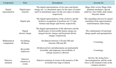
Table 1. The computer simulation process of physical reality.

Components Parts Descriptions Account for

Digital representation

Digital space structure

The digital representations of rest mass and kinetic energy are 1 as attachment space for the space of matter and 0 as detachment space for the zero-space of matter,

respectively

Higgs field, reverse Higgs field, quantum mechanics, special relativity, force fields, dark matter,

baryonic matter

Digital spin

The digital representations of the exclusive and the inclusive occupations of positions are 1/2 spin

fermion and integer spin boson, respectively

The expanding universe by spatial translation from supersymmetry

transformation, dark energy

Digital electric charge

The digital representations of the allowance and the disallowance of irreversible kinetic energy are integral electric charges and fractional electric

charges, respectively

The confinements of fractional charge quarks and quasiparticles

Mathematical computation

Oscillating M-theory

Oscillations between 11D and 10D and

between 10D and 4D Cosmology

Reversible multiverse

All physical laws and phenomena are permanently reversible, and temporary irreversibility of

entropy increase is allowed

Cosmology

Selective retention

Selective retention of events

Selective retention of events in the narrative of the reversible four-stage evolution

Gravity, the strong force, electromagnetism, and the weak force as the retained events in the

common narrative

charge transformation to become the 10D dual string universe, which in turn can return to the 11D dual membrane universe that in turn can return to the zero-energy universe as Figure 2.

5. Summary

This paper posits that we are living in a computer simulation to simulate physical reality which has the same computer simulation process as virtual reality (computer-simulated reality). Both computer simulation processes for physical reality and virtual reality involve the digital representation of data, the mathematical computation of the digitized data in geometric formation and transformation in space-time, and the selective retention of events in a narrative. We are living in a computer simulation consisting of the digital representation component, the mathematical computation component, and the selective retention component.

For the digital representation component of physical reality, the three intrinsic data (properties) are rest mass- kinetic energy, electric charge, and spin which are represented by the digital space structure, the digital electric charge, and the digital spin, respectively. For the digital space structure, the digital representations of rest mass and kinetic energy are 1 as attachment space for the space of matter and 0 as detachment space for the zero- space of matter, respectively. Attachment space and detachment space are the origins of the Higgs field and the reverse Higgs field, respectively. The combination of n units of attachment space as 1 and n units of detachment space as 0 brings about the three digital structures: binary partition space (1)n(0)n, miscible space (1 + 0)n, and

binary lattice space (1 0)n to account for quantum mechanics, special relativity, and the force fields, respectively.

For the digital spin, the digital representations of the exclusive and the inclusive occupations of positions are 1/2 spin fermion and integer spin boson, respectively. The exclusion-inclusion brings about spatial translation by the supersymmetry transformations between fermion and boson. For the digital electric charge, the digital re-presentations of the allowance and the disallowance of irreversible kinetic energy are integral electric charges and fractional electric charges, respectively. The disallowance of irreversible kinetic energy of fractional electric charges brings about the confinement of fractional electric charges for quarks and quasiparticles in hadrons and two dimensional systems, respectively.

supersym-metry transformation. Without the digital electric charge, fractional charge quarks would have not existed to constitute nucleus in atom.

The mathematical computation involves the reversible multiverse and oscillating M-theory as oscillating membrane-string-particle whose space-time dimension (D) number oscillates between 11D and 10D and be-tween 10D and 4D. Space-time dimension number bebe-tween 10 and 4 decreases with decreasing speed of light, decreasing vacuum energy, and increasing rest mass. The mathematical computation component explains cos-mology. Gravity, the strong force, electromagnetism, and the weak force in our universe are the retained events during the four-stage evolution of our universe, and are unified by the common narrative of the evolution in the selective retention component.

Conventional physics cannot explain the reality of quantum mechanics easily. Conventional physics cannot explain the origins of the confinement of quarks and the fractional charges of quasiparticles. The geometry in conventional physics is fixed M-theory which has no experimental proof. Conventional physics cannot unify the four force fields. Conventional physics cannot explain physical reality clearly, while computer-simulated phys-ics can explain physical reality clearly by using the computer simulation process consisting of the digital repre-sentation component, the mathematical computation component, and the selective retention component. We are living in a computer simulation. Table 1 is the summary of the computer simulation process of physical reality

References

[1] Bostrom, N. (2003) Philosophical Quarterly, 53, 243-255. http://dx.doi.org/10.1111/1467-9213.00309

[2] Chung, D. and Krasnoholovets, V. (2013) Journal of Modern Physics, 4, 27-31.

http://dx.doi.org/10.4236/jmp.2013.44A005

[3] Chung, D. (2015) Journal of Modern Physics, 6, 1820-1832. http://dx.doi.org/10.4236/jmp.2015.613186

[4] Chung, D. (2016) Journal of Modern Physics, 7, 642-655. http://dx.doi.org/10.4236/jmp.2016.77064 [5] Chung, D. (2016) Journal of Modern Physics, 7, 1150-1159.

[6] Chung, D. (2015) Journal of Modern Physics, 6, 1249-1260. http://dx.doi.org/10.4236/jmp.2015.69130

[7] Chung, D. and Krasnoholovets, V. (2007) Scientific Inquiry, 8, 165-182.

[8] Chung, D. (2015) Journal of Modern Physics, 6, 1189-1194. http://dx.doi.org/10.4236/jmp.2015.69123

[9] Chung, D. and Krasnoholovets, V. (2013) Journal of Modern Physics, 4, 77-84.

http://dx.doi.org/10.4236/jmp.2013.47A1009

[10] Woit, P. (2006) Not Even Wrong: The Failure of String Theory and the Search for Unity in Physical Law. Basic Books, New York.

[11] Weinberg, S. (1989) Review Modern Physics, 61, 1-23. http://dx.doi.org/10.1103/RevModPhys.61.1

[12] Chung, D. and Hefferlinm, R. (2013) Journal of Modern Physics, 4, 21-26.

http://dx.doi.org/10.4236/jmp.2013.44A004

[13] Diaz, B. and Rowlands, P. (2003) American Institute of Physics Proceedings of the International Conference of Com-puting Anticipatory Systems, Liege, 11-16 August 2003, 203-218.

[14] Bell, J. (1964) Physics, 1, 195-199.

[15] Mahler, D., et al. (2016) Science Advances, 2, e1501466.

[16] Penrose, R. (2000) Wavefunction Collapse as a Real Gravitational Effect. In: Fokas, A., Grigoryan, A., Kibble, T. and Zegarlinski, B., Eds., Mathematical Physics 2000, Imperial College, London, 266-282.

http://dx.doi.org/10.1142/9781848160224_0013

[17] Bounias, M. and Krasnoholovets, V. (2003) The International Journal of Systems and Cybernetics, 32, 1005-1020.

[18] Chung, D. (2014) Journal of Modern Physics, 5, 1234-1243. http://dx.doi.org/10.4236/jmp.2014.514123

[19] Chung, D. (2014) Journal of Modern Physics, 5, 464-472. http://dx.doi.org/10.4236/jmp.2014.56056

[20] Jarosik, N., Bennett, C.L., Dunkley, J., Gold, B., Greason, M.R., Halpern, M., et al. (2011) The Astrophysical Journal

Supplement Series, 192, 14. http://dx.doi.org/10.1088/0067-0049/192/2/14

[21] Chung, D. (2014) Journal of Modern Physics, 5, 1467-1472. http://dx.doi.org/10.4236/jmp.2014.515148

[22] Chung, D. (2014) International Journal of Astronomy and Astrophysics, 4, 374-383.

http://dx.doi.org/10.4236/ijaa.2014.42032