Learning backward induction: a neural network agent approach

Munich Personal RePEc Archive

Learning backward induction: a neural

network agent approach

Leonidas, Spiliopoulos

12 September 2009

Online at

https://mpra.ub.uni-muenchen.de/40621/

Learning backward induction: a neural network agent approach

Leonidas Spiliopoulos

Abstract

This paper addresses the question of whether neural networks (NNs), a realistic cognitive model of human information processing, can learn to backward induce in a two-stage game with a unique subgame-perfect Nash equilibrium. The NNs were found to predict the Nash equilibrium approximately 70% of the time in new games. Similarly to humans, the neural network agents are also found to suffer from subgame and truncation inconsistency, supporting the contention that they are appropriate models of general learning in humans. The agents were found to behave in a bounded rational manner as a result of the endogenous emergence of decision heuristics. In particular a very simple heuristicsocialmax, that chooses the cell with the highest social payoff explains their behavior approximately 60% of the time, whereas theownmaxheuristic that simply chooses the cell with the maximum payoff for that agent fares worse explaining behavior roughly 38%, albeit still significantly better than chance. These two heuristics were found to be ecologically valid for the backward induction problem as they predicted the Nash equilibrium in 67% and 50% of the games respectively. Compared to various standard classification algorithms, the NNs were found to be only slightly more accurate than standard discriminant analyses. However, the latter do not model the dynamic learning process and have an ad hoc postulated functional form. In contrast, a NN agent’s behavior evolves with experience and is capable of taking on any functional form according to the universal approximation theorem.

Key words: Agent based computational economics; Backward induction; Learning models; Behavioral game theory; Simulations; Complex adaptive systems; Artificial intelligence; Neural networks

1. Introduction

This paper investigates the potential of neural networks to learn the sophisticated concept of backward induction. This is of particular interest as failures of backward induction reasoning in humans have been documented in many papers e.g. Binmore et al. (2002) and Johnson et al. (2002). Neural networks in conjunction with a backpropagation learning algorithm were chosen to model the learning agents as they are considered to be the most biologically plau-sible cognitive model of parallel information processing, approximating real neuronal adaptation in the human mind (Robinson, 2000; Zipser & Andersen, 1988; Mazzoni et al., 1991; Kettner et al., 1993; Lehky & Sejnowski, 1988; Dror & Gallogly, 1999).

The universal approximation theorem (Hornik, 1991; Cybenko, 1989; Funahashi, 1989) states that given a large enough finite number of neurons a single layer neural network (NN) is a universal function approximator i.e. it will be able to approximate any function, with any desired level of accuracy. Modeling agents as neural networks evades the problem of ad hoc specification of the exact functional form of the learning model. Instead, they evolve endogenously according to the backpropagation algorithm that adjusts the neural networks’ parameters in the direction of error minimization starting from an initial non-informative random state. However, as the backpropagation algorithm is a gradient descent approach it is possible for it to become mired in a local rather than global optimum, so that the NN agents will likely eventually learn to behave in a bounded-rational manner as is observed in human behavior.

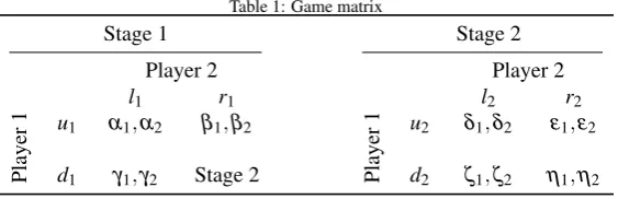
Table 1: Game matrix

Stage 1 Stage 2

Player 2 Player 2

l1 r1 l2 r2

Player

1 _u

1 α1,α2 β1,β2

Player

1 _u

2 δ1,δ2 ε1,ε2

d1 γ1,γ2 Stage 2 d2 ζ1,ζ2 η1,η2

equilibrium, and to observe how closely correlated these agents’ behavior was to humans’. Spiliopoulos (2009) has extended their work by examining neural network agents learning to play all possible strategic types of 3×3 games. Another paper (Cho & Sargent, 1996) incorporating neural networks in game theory uses perceptrons, or simple NNs, as a way of modeling bounded rational behavior in repeated situations, such as a repeated prisoner’s dilemma.1

2. Methodology

2.1. Game sampling

The class of games studied in this paper involve two players and two stages, each with a 2×2 action space and a unique subgame-perfect Nash Equilibrium, as shown in Table 1. Each payoff is drawn randomly from a uniform distribution with support from 0 to 100. For each stages, Player 1 has available actions upanddown, denoted by

us anddsand Player 2 actionsleft, ls, andright, rs. If in the first stage the players choosed1andr1then the game proceeds to the second stage.

2.2. Introduction to neural networks

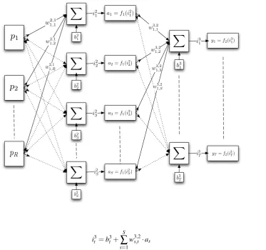
A detailed technical diagram of the topology of the feedforward neural networks employed in this study is given in Figure 1. The first layer (leftmost in the diagram) is the input layer and each input neuron is denoted bypr where

r=1, ...,R, and each prneuron inputs the payoff for a specific player for each cell of the game. The second layer2,

referred to as the hidden layer, consists ofSneurons, each of which is connected to all the input neurons, resulting in a total ofR·Sconnections between the first and second layers. Each connection is associated with a weight,w2s,r,1, with

s,rdenoting a connection from therthneuron to thesthneuron and where the superscript 2,1 represents that these weights are between the first and second layers of the NN. The activation of each neuron in the second layer,i2_s, is the summation of the product of the inputs and their corresponding weights plus a constant or bias,b2_s i.e. for each ofS

neurons in the second or hidden layer:

i2_s=b2_s+

R

∑

r=1

w2_r,s,1·pr (1)

These inputs are now passed through a non-linear function, f1(is) =2·(1+e−2i

2

s₎−1_{−1 , in this particular case the} hyperbolic tangent sigmoid (or tansig) function, which maps values from−∞to+∞to the interval(−1,1). The resulting outputs,as, are passed to the the final or output layer which is comprised ofT neurons. Each neuron in

the output layer is associated with a single cell in the payoff matrix and the output value represents the strength with which the NN associates that cell with the Nash equilibrium. Again each neuron in the output layer is connected to every neuron in the second layer with connection weights,w3_s,t,2. The input to eacht neuron is the summation of product of the outputs,as, and the corresponding weights,w3s,t,2plus a biasb3t:

1_{They show that even the simplest NN, a single perceptron, is capable of implementing trigger strategies in a repeated prisoner’s dilemma}

game and of supporting all subgame perfect payoffs. They also prove that only a slightly more complicated network is capable of supporting all equilibrium payoffs in a general 2×2 game.

2_{For simplicity, the network presented has only one hidden layer however some of the NNs in this paper will employ more than one hidden}

layer, each with identical structural and functional properties.

Figure 1: Detailed structure and topology of feedforward neural networks

w2,1

1,1

p

p

pR

w2,1 1,2

w2,1 1,R

�

�

�

�

a1=f1(i21)

a₂=f₁(i2 2)

a3=f1(i 2 3)

aS=f₁(i2S)

b2 1 b2 2 b2 3 b2 S

�

�

1,1

w3,2 1,2

w3,2 1,3

w3,2₁ ,S

b3 1

b3

T

y1=f2(i 3 1)

yT=f2(i 3 T) i2 1 i2 2

i2₃

i2_S

i3

1

i3 T

i_t3=b_t3+

S

∑

s=1

w3_s,t,2·as (2)

These inputs are transformed by the transfer function of the output layer neurons which in this case is simply a linear functionf2, such that the final outputs of the NN are defined byyt=f2(i3t) =i3t.

In processing the data, information flows forwards through the neural network, from left to right in the diagram, whereas by contrast the standard learning mechanism of a NN implicitly uses a backward flowing system, as exem-plified by its name, the backpropagation rule. After making a decision the NN compares the values of the neurons at the output layer to the desired values and makes adjustments to all the connection weights in such a way that would reduce the error of the NN. The backpropagation learning rule uses the chain rule to assign the contribution of each neuron to the observed error, from which it is then possible to extract the necessary information regarding how to change each connection weight in order to reduce the overall error. Each connection weight is changed according to a gradient descent method with the intent that the network successively approaches a state where the error function attains a minimum. However, this algorithm is not immune to the possibility of settling on a local rather than global minimum. A detailed mathematical presentation of the backpropagation algorithm is given in Appendix A.

2.3. Simulations, models and heuristics

Four different agent simulations were run using standard feedforward neural networks of different topologies, denoted byνlwherelis the number of hidden layers. For each simulation, ten different networks of the same topology

were trained with different initial weights, emulating players with different initial, random weights. This will allow the examination of how important prior knowledge may be to the learning process and whether different types of players emerge in the simulation. Although the number of hidden layers of the NNs is varied across simulations, the

number of neurons in each hidden layer is always ten.3_{The input layers of the NNs consist of 14 neurons, with each} neuron entering each player’s payoffs from each cell in the game matrices. The output layer consisted of 7 linear transfer function neurons each one representing a cell in the payoff matrices and the desired output was simply a 7-tuple vector with values of one for the cells which were the NE and zero otherwise.4 The final payoff cell chosen by a network was assumed to be the one whose corresponding output neuron had the maximum value compared to the rest.

All the NN agents learned via a batch backpropagation algorithm incorporating an adaptive learning rate param-eter . One generation of learning, or batch, consisted of the presentation of 1000 different games, and the training process was terminated when the cross-validation MSE of the network’s output did not improve for 100 consecutive generations. Cross validation was employed as an early stopping procedure to avoid overfitting and provide an upper bound for neural network performance. All testing was done on sets of 2500 out of sample games in order to test the networks’ ability to generalize.

To provide benchmarks against which to compare the NNs generalizing ability, six other standard classification algorithms will be estimated from the data and the performance of two simple heuristics will also be investigated. The classification algorithms are the linear, quadratic, logistic and canonical linear discriminant analyses (DA), nearest neighbor, and a classification tree, all of which were implemented in Stata 10 except for the latter which was estimated in Matlab.

Two simple heuristics that make unique predictions for the whole set of games are simply choosing the cell with the maximum own payoffownmax, and a heuristic that picks the cell with the maximum social payoff,socialmax.

2.4. Performance testing

The networks’ performances were documented for four different test sets as presented in Table 2. Thecomplete

test set is comprised of new games of exactly the same structure as the ones presented during the training session. Three other test sets that will be used are inspired by Harsanyi & Selten (1988) and their proof that subgame perfec-tion in finite games with perfect informaperfec-tion is equivalent to compliance with three principles, raperfec-tionality, subgame consistency and truncation consistency. Subgame consistency states that a player’s behavior in a subgame does not depend on the position of the subgame within the encompassing game. Truncation consistency occurs if replacing a subgame with its equilibrium payoff does not alter players’ behavior anywhere else in the game.

Thetruncatedset was created by keeping the first stage of the games in the complete set as is, but replacing one of the cells in the second stage with the Nash equilibrium of that stage, whilst setting all other payoffs to zero. The

truncated/last stageset simply moved all the non-zero payoffs from thetruncatedset games to the final stage of the game, whilst all payoffs in the first stage were set to zero. Thelast stagedataset is created by taking the second stage of thecompletetest set games and setting all payoffs in the first stage equal to zero, thereby testing whether the NN agents learned to solve for the Nash equilibrium of the second stage game, a necessary subgoal to successfully apply backward induction.

3. Results

3.1. Comparison of NN topologies

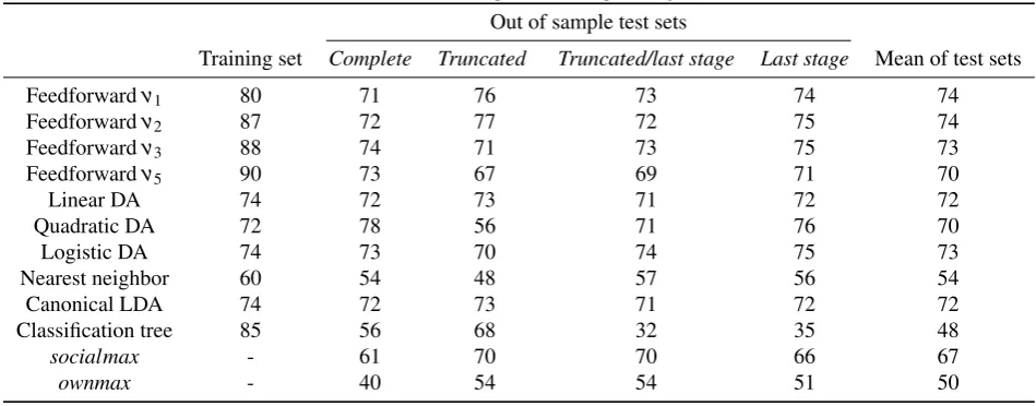
Table 2 highlights some of the main results from the analyses of the various neural network agents, where the data is derived from by the performance of the ten trained neural networks in each simulation. This aggregation is justified by the finding in Section 3.5 that the NNs behave very similarly after training implying little impact of the initial weights.

Comparing the results between the various neural network topologies the success rate on the training set was high ranging from 80-90%. Also, there do not exist significant differences in the mean performance on all the test sets, as they range from 74% for theν1andν2networks to 70% forν5. As the number of layers used in the feedforward networks increases performance on the training set also increases as expected, however performance on the tests sets

3_{Simulations of neural networks with more neurons were at best not found to significantly improve performance, and often degraded}

perfor-mance due to overfitting.

4_{Note that this is a stricter prediction criterion than asking the neural network to simply play the NE strategy.}

Table 2: Neural network performance at predicting NE

Out of sample test sets

Training set Complete Truncated Truncated/last stage Last stage Mean of test sets

Feedforwardν1 80 71 76 73 74 74

Feedforwardν2 87 72 77 72 75 74

Feedforwardν3 88 74 71 73 75 73

Feedforwardν5 90 73 67 69 71 70

Linear DA 74 72 73 71 72 72

Quadratic DA 72 78 56 71 76 70

Logistic DA 74 73 70 74 75 73

Nearest neighbor 60 54 48 57 56 54

Canonical LDA 74 72 73 71 72 72

Classification tree 85 56 68 32 35 48

socialmax - 61 70 70 66 67

ownmax - 40 54 54 51 50

is decreasing. This implies that using more than one hidden layer is not necessary and only leads to overfitting to the training sample. Given the close performance of all the neural networks in conjunction with the fact that theν1agents have significantly fewer parameters, all discussion henceforth will refer only to this network topology for the sake of brevity.

3.2. Comparison of NNs to standard classification algorithms and heuristics

Comparison of theν1agents’ performance and the standard classification algorithms reveals that the NNs were the most successful in the out of sample test sets, as would be expected given their flexibility. Upon closer inspec-tion however, four of the classificainspec-tion algorithms had near identical performance, the linear, quadratic, logistic and canonical discriminant analyses. The most intriguing result is that the linear DA performed very well compared to the other discriminant analyses, demonstrating that non-linearity was not important. The worst performers were the classification tree and the nearest neighbor algorithm, whose performance was significantly lower than that of the other models.

Focusing attention on the two simple heuristics, the results are particularly impressive given their simplicity. Most striking is the performance of thesocialmaxheuristic which correctly performs predicts the Nash equilibrium in 67% of all the test set games, compared to 74% for the sophisticatedν1 neural networks. The greedyownmax heuristic which completely ignored opponents’ payoffs still performed relatively well given its simplicity and low information requirements, with a mean test set performance of 50%. These results imply that thesocialmaxheuristic is ecologically valid for this type of problem. The intuition behind its excellent performance is that the higher the payoff of an action the more likely it is to be the Nash equilibrium action for a player, therefore choosing the cell with maximum social payoffs very often coincides with the Nash equilibrium. This result agrees with the conclusions of research on fast and frugal heuristics (Gigerenzer, 2000; Gigerenzer & Selten, 2001), specifically that ecologically valid heuristics can perform as well or even better than significantly more sophisticated models of behavior.

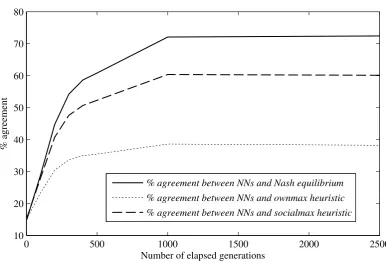
Although the success of thesocialmaxheuristic in predicting the NE is high, this does not necessarily imply that this heuristic is a good approximator of the NNs’ behavior. The two lower time series in Figure 2 graph the percentage of games for which the NN agents and the two heuristics make the same predictions as a function of the elapsed generations of learning experience of the agents. Thesocialmaxheuristic is a much more accurate approximator of the NN agents play as it correctly predicts their behavior at a limiting value of 60%, compared to just under 40% for theownmaxheuristic.

This result is of great importance because if it had arisen in an experimental study, then it would be tempting to attribute altruistic behavior to the players as they seem to care not only about their own payoffs but also those of their opponents. This conclusion however would be erroneous as there exist no altruistic incentives in the learning mechanism of the neural networks employed in this study. This highlights the danger of attributing specific types of

Figure 2: Agreement between NN behavior and various other times series

0 500 1000 1500 2000 2500

10 20 30 40 50 60 70 80

Number of elapsed generations

% agreement

% agreement between NNs and Nash equilibrium

% agreement between NNs and ownmax heuristic

% agreement between NNs and socialmax heuristic

behavior to experimental subjects only on the basis of their observable actions. In this case, it is the ecological validity of thesocialmaxheuristic which induces it to endogenously emerge in the NN agents’ behavior. The possibility that the ecological validity of certain types of behavior have been misattributed to built-in incentives or motives of agents has not been addressed adequately in the literature, and is a distinction that deserves further attention.

Finally, it should be noted that a significant methodological advantage of modeling agents as neural networks instead of the classification algorithms or heuristics, is that they explicitly model the learning process increasing their plausibility and realism, whereas the latter remain silent with regards the dynamic learning process.

3.3. Detailed analysis ofν1agents’ performance

Theν1agents predict the Nash equilibrium for 71% of the games in the complete test set. The evolution of the agents’ mean performance on all the test sets is shown in Figure 2. Learning at the beginning of the training phase is initially very fast but progressively slows down as the NNs’ experience increases, culminating in a final performance above 70%. The performance for thetruncated game set rises to 76%, as a result of directly providing the Nash equilibrium of the second stage. This implies that the NNs have not perfectly learned to solve for the second stage NE, otherwise there should be no discernible change in performance. This is further validated by the performance on thelast stagetest set which directly examines the degree to which the NNs are capable of solving for the NE of the second stage. The performance of 74% on this test set although quite good confirms that the NNs have not managed to perfectly learn the importance of backward induction.

Finally, it is interesting to note that the NNs performed almost equally well both on thecomplete test set and thelast stagetest set. Hence, the decision rules that have endogenously emerged in the NNs are equally capable of predicting the NE both in games with a single stage not requiring backward induction, as well as two-stage games requiring it, as long as the games exhibit a unique pure strategy Nash equilibrium.

3.4. Subgame and truncation consistency

Experimental tests of subgame and truncated consistency in Binmore et al. (2002) reveal that human subjects often violate these principles. Subgame consistency is tested in this paper by comparing the agents’ behavior in

Table 3: Compliance with notions of subgame and truncation consistency as % of NN agents’ actions Subgame Truncation

Feedforwardν1 69.24 76.84

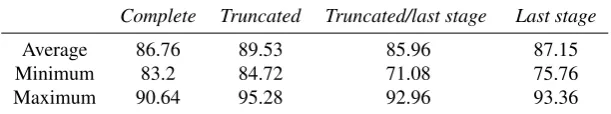
Table 4: Percentage agreement between differentν1NN agents

Complete Truncated Truncated/last stage Last stage

Average 86.76 89.53 85.96 87.15

Minimum 83.2 84.72 71.08 75.76

Maximum 90.64 95.28 92.96 93.36

thetruncated andtruncated/last stage test sets. As documented in Table 3, the NNs’ behavior is compatible with subgame consistency only 69% of the time, indicating that similarly to humans these agents also violate this principle. Truncation inconsistency was also found as comparing thecompleteset with thetruncatedtest set led the NN agents to change their behavior in roughly 23% of the games.

It should be noted that by construct thesocialmaxandownmaxheuristics do not suffer from subgame inconsis-tency, however they are vulnerable to truncation inconsistency. Therefore despite the appeal of thesocialmaxheuristic as exhibited by its ability to approximate the NNs quite well, it does not capture the truncation inconsistency that is found both in humans and the NN agents.

In conclusion, the evidence supports that the NN agents exhibit the same inconsistencies that experimental subjects do, increasing their credibility as realistic learning models of human behavior.

3.5. Agent heterogeneity

The ten NN agents were trained starting from different initial values, therefore an examination into the heterogene-ity of their behavior after training is warranted. One possibilheterogene-ity is that each NN may have evolved into a different type of player as a result of these different initial conditions. However the longer the training phase the less should be the dependence upon the initial conditions, unless the NNs have converged on significantly different local minima. Table 4 shows the percentage agreement of all possible pairwise comparison between the ten NNs for each of the test sets. For all the test sets the average agreement is high, ranging from 85.96% to 89.53%, and the maximum and minimum values of agreement are quite tightly distributed around this mean. In conclusion, the NN agents have evolved very similarly despite different initial conditions and show relatively little between-agents heterogeneity.

4. Conclusion

This paper has shown that applying backward induction to solve for the subgame perfect NE in two-stage games is not trivial even for the processing capabilities of a neural network. Although perfect performance is theoretically possible the NNs were found to behave in a bounded rational way in agreement with documented human behavior, likely the result of the gradient descent backpropagation method settling in a local rather than global optimum. Despite this, the neural networks performed quite well predicting the Nash equilibrium of new games roughly 71% of the time. Also, the NNs and experimental subjects both exhibited the same violations of backward induction, namely that of truncation and subgame consistency.

The evolved behavior of the NNs appears to have great portability and robustness as it is capable of predicting equally well in environments where backward induction is not necessary i.e. single stage games, as long as the games have a unique pure strategy Nash equilibrium.

Thesocialmaxheuristic that predicted the Nash equilibrium as the cell with the highest social payoff was found to be ecologically valid for games with a single pure strategy Nash equilibrium, as it was correct in 67% of all test games. This heuristic also explained the behavior of the NN agents quite well as it made the same prediction approximately 60% of the time.

The NN agents were found to perform slightly better than other classification techniques such as linear discrimi-nant analysis in recognizing the Nash equilibrium. However, the former are preferable on two grounds. Firstly, they

model the complete dynamic learning process using a plausible cognitive model of information processing of the human mind. Secondly, the exact functional form of the agents’ behavior emerges endogenously as a consequence of the learning procedure rather than being postulated ad hoc.

Concluding, the neural network agents were proven to be valuable learning models as their behavior was qualita-tively very similar to human behavior, whilst also being more biologically plausible than other models.

References

K. Binmore, et al. (2002). ‘A Backward Induction Experiment’.Journal of Economic Theory104(1):48–88.

I. Cho & T. Sargent (1996). ‘Neural Networks for Encoding and Adapting in Dynamic Economies’. Handbook of Computational Economics

1:441–470.

G. Cybenko (1989). ‘Approximation by superpositions of a sigmoidal function’.Mathematics of Control, Signals and Systems2:303–314. I. E. Dror & D. P. Gallogly (1999). ‘Computational analyses in cognitive neuroscience: In defense of biological implausibility’. Psychonomic

Bulletin & Review6(2):173–182.

K. Funahashi (1989). ‘On the approximate realization of continuous mappings by neural networks’.Neural Networks2:183–192. G. Gigerenzer (2000).Adaptive thinking: Rationality in the real world. Oxford University Press, New York.

G. Gigerenzer & R. Selten (eds.) (2001).Bounded rationality: The adaptive toolbox. MIT Press, Cambridge, MA. J. C. Harsanyi & R. Selten (1988).A General Theory of Equilibirum Selection in Games. MIT Press, Cambridge, MA. K. Hornik (1991). ‘Approximation capabilities of multilayer feedforward networks’.Neural Networks4:251–257.

E. J. Johnson, et al. (2002). ‘Detecting failures of backward induction: Monitoring information search in sequential bargaining experiments’.

Journal of Economic Theory104:16–47.

R. Kettner, et al. (1993). ‘A neural network model of cortical activity during reaching’.Journal of Cognitive Neuroscience5:14–33.

S. R. Lehky & T. J. Sejnowski (1988). ‘Network model of shape-from-shading: Neural function arises from both receptive and projective fields’.

Nature333:452–454.

P. Mazzoni, et al. (1991). ‘A more biologically plausible learning rule than backpropagation applied to a network model of cortical area 7a’.

Cerebral Cortex1:293–307.

T. Robinson (2000). ‘Biologically Plausible Back-Propagation’. Tech. rep., Victoria University of Wellington.

D. Sgroi & D. J. Zizzo (2007). ‘Neural networks and bounded rationality’.Physica A: Statistical Mechanics and its Applications375(2):717–725. L. Spiliopoulos (2009). ‘Neural Networks as a Learning Paradigm for General Normal Form Games’. SSRN eLibrary

-http://ssrn.com/paper=1447968.

D. Zipser & R. A. Andersen (1988). ‘A back-propagation programmed network that simulates response properties of a subset of posterior parietal neurons’.Nature331:679–684.

A. Technical presentation of the NN backpropagation algorithm

Knowledge is stored in NNs by the weights and biases of all the neurons, which is why it is referred to as distributed knowledge since it is not localized in any specific region of the NN structure. Hence, learning in a NN is accomplished through the updating of the weights and biases after presentation of each set of inputs, in this case each game’s payoff matrix. In supervised learning, for each gamegand each set of inputs,P={p1,g, ...,pR,g}, there exists a set of ideal

outputs,Z ={z1,g, ...,zT,g}, denoting whether the corresponding cell is the Nash equilibrium or not. The desired

output corresponding to the cell which is the Nash equilibrium is encoded with a value of 1, or 0 otherwise.

In the case of batch training which is used in this paper, all the 1000 training games are presented in a single batch to the neural network and the mean square error over all games,E, is computed according to:

E=1

2·

G

∑

g=1

(

T

∑

t=1

(zt,g−yt,g)2) (3)

The neural network weights will then be adjusted as explained below, after which another batch (with exactly the same inputs as the previous batch) will be presented to the NN. This process is repeated until the cross validation criterion is met and training ends. The most common learning algorithm used in training NNs is the backpropagation algorithm which uses a gradient descent technique. After the presentation of each set of inputs the weights are changed according to the following equation:

�w·_·,_,·_·=−η ∂E ∂w··,,··

(4)

This is a gradient descent technique as the updating of the weights depends on the negative of the gradient of the error function and on its magnitude, whereη is referred to as the step size (or learning rate) that governs the magnitude of the change in the weights. Hence, weights will be changed in the direction which reduces the error,E, and the magnitude of the change will also be related to the sensitivity of the error function to small changes in the weight. In standard backpropagationηis a constant, whereas backpropagation with an adaptive learning parameter scalesηupwards if the mean square errorEdecreased in the previous batch presentation or scaled downwards ifE

increased. The necessary algebra to derive∂E_{/∂wfor both output layer and hidden layer neurons is presented below.}

In more detail, for weights in the output layer, using the chain rule leads to the following derivation:

∂E ∂w3_s,t,2 =

G

∑

g=1

∂E ∂y_t,g

∂yt,g

∂i3

t

∂i3_t

∂w3_s,t,2 (5)

However, from equation 2 it is clear that:

∂i_t3

∂w3_s,t,2=as (6)

and from equation 3:

∂E ∂yt,g= (

yt,g−zt,g) (7)

Substituting these equations into equation 5 and recognizing that for a linear transfer function f₂�(i3_t) =1 results in:

∂E ∂w3_s,t,2 =

G

∑

g=1

(yt,g−zt,g)as (8)

The necessary calculations for weights in hidden layers is more involved as the desired output of such neurons is not immediately available as is the case for output layer neurons. Using the chain rule, the analog to equation 5 for a hidden layer neuron is:

∂E ∂w2s,r,1

=

G

∑

g=1

T

∑

t=1

∂E ∂yt,g

∂y_t,g ∂as

∂as

∂w2s,r,1

(9)

This equation now has a summation of terms overt since hidden layer weights can affect the error of the NN through all the output layer neurons due to the propagation of the effect ofw2_s,r,1through the interconnections between thesthneuron and allT neurons in the output layer. The derivative of the output of thesthneuron with respect to the weight under investigation is given by:

∂as

∂w2s,r,1

=prf

�

1(i2s) (10)

The derivative of the error function w.r.t. the output of each final layer neuron,∂E_{/∂yt,g, is still given by equation 7.}

Finally, the derivatives of the output of each final layer neuron w.r.t. the output of each hidden layer neuron are given by:

∂yt,g

∂as

=w_t,s3,2f₂�(i_t3) (11)

In conclusion, substituting equations 10, 7, 11 and f₂�(i3_t) =1 into equation 9 leads to the following equation:

∂E ∂w2s,r,1

=

G

∑

g=1

T

∑

t=1

prf

�

1(i2s)(yt,g−zt,g)wt,s3,2 (12)