Correct Classification Rates in Multi Category Discriminant Analysis of Spatial Gaussian Data

http://dx.doi.org/10.4236/ojs.2015.51003

Correct Classification Rates in

Multi-Category Discriminant Analysis

of Spatial Gaussian Data

Lina Dreižienė

1,2

, Kęstutis Dučinskas

1

, Laura Paulionienė

1

1_{Department of Mathematics and Statistics, Klaipėda University, Klaipėda, Lithuania} 2_{Institute of Mathematics and Informatics, Vilnius University, Vilnius, Lithuania}

Email: [email protected], [email protected], [email protected]

Received 28 December 2014; accepted 17 January 2015; published 22 January 2015

Copyright © 2015 by authors and Scientific Research Publishing Inc.

This work is licensed under the Creative Commons Attribution International License (CC BY).

http://creativecommons.org/licenses/by/4.0/

Abstract

This paper discusses the problem of classifying a multivariate Gaussian random field observation into one of the several categories specified by different parametric mean models. Investigation is conducted on the classifier based on plug-in Bayes classification rule (PBCR) formed by replacing unknown parameters in Bayes classification rule (BCR) with category parameters estimators. This is the extension of the previous one from the two category cases to the multi-category case. The novel closed-form expressions for the Bayes classification probability and actual correct classifi-cation rate associated with PBCR are derived. These correct classificlassifi-cation rates are suggested as performance measures for the classifications procedure. An empirical study has been carried out to analyze the dependence of derived classification rates on category parameters.

Keywords

Gaussian Random Field, Bayes Classification Rule, Pairwise Discriminant Function, Actual Correct Classification Rate

1. Introduction

Much work has been done concerning the error rates in two-category discrimination of uncorrelated observa-tions (see e.g. [1]). Several methods for estimations of the error rates in discriminant analysis of spatial data have been recently proposed (see e.g. [2] [3]).

known normal populations by single linear discriminant function. Techniques for multi-category probability es-timation by combining all pairwise comparisons are investigated by several authors (see e.g. [5]). Empirical comparison of different methods of error rate estimation in multi-category linear discriminant analysis for mul-tivariate homoscedastic Gaussian data was performed by Hirst [6]. Bayesian multiclass classification problem for correlated Gaussian observation was empirically studied by Williams [7]. The novel model-free estimation method for multiclass conditional probability based on conditional quintile regression functions is theoretically and numerically studied by Xu [8]. Correct classification rates in multi-category classification of independent multivariate Gaussian observations were provided by Schervish [9]. We generalize results of above to the prob-lem of classification of multivariate spatially correlated Gaussian observations.

We propose the method of multi-category discriminant analysis essentially exploiting the Bayes classification rule that is optimal in the sense of minimum misclassification probability in case of complete statistical certainty (see [10], chapter 6). In practice, however, the complete statistical description of populations is usually not possible. Then having training sample, parametric plug-in Bayes classification rule formed by replacing un-known parameters with their estimators in BCR is being used.

Šaltytė and Dučinskas [11] derived the asymptotic approximation of the expected error rate when classifying the observation of a scalar Gaussian random field into one of two classes with different regression mean models and common variance. This result was generalized to multivariate spatial-temporal regression model in [12]. However, the observations to be classified are assumed to be independent from training samples in all publica-tion listed above. The assumppublica-tion of independence for the classificapublica-tion of scalar GRF observapublica-tions was re-moved by Dučinskas [2]. Multivariate two-category case has been considered in Dučinskas [13]and Dučinskas and Dreižienė [14]. Formulas for the error rates for multiclass classification of scalar GRF observation are de-rived in [15]. The authors of the above papers have been focused on the maximum likelihood (ML) estimators because of tractability of the covariance matrix of these estimators. In the present paper, we extend the investi-gation of the performance of the PBCR in multi-category case. The novel closed form expressions for the actual correct classification rate (ACCR) are derived.

By using the derived formulas, the performance of the PBR is numerically analyzed in the case of stationary Gaussian random field on the square lattice with the exponential covariance function. The dependence of the correct classification rate and ACCR values on the range parameter is investigated.

The rest of the paper is organized as follows. Section 2 presents concepts and notions concerning BCR ap-plied to multi-category classification of multivariate Gaussian random field (MGRF) observation. Bayes proba-bility of correct classification is derived. In Section 3, the actual correct classification rate incurred by PBCR is considered and its closed-form expression is derived. Numerical examples, based on simulated data, are pre-sented in Section 4, in order to illustrate theoretical results. The effect of the values of range parameter on the values of ACCR is examined.

2. The Main Concepts and Definitions

The main objective of this paper is to classify a single observation of MGRF

{

Z s

( )

:s∈ ⊂D R2

}

into one of L categories, say Ω₁,,ΩL.

The model of observation Z s

( )

in category Ω_l

(

l=1,,L

)

is

( )

l

(

; l

) ( )

Z s =µ s B +ε s .

Here µ_l represents a mean component and B_l is a matrix of parameters. The error term is generated by

p-dimensional zero-mean stationary GRF

{

ε

( )

s :s∈D

}

with covariance function defined by model for all

s, u∈D

( ) ( )

{

}

(

)

cov ε s ,ε u =r s u− Σ,

where r s u

(

−

)

is the spatial correlation function and Σ is the variance-covariance matrix with elements

{ }

σ

ij . So we have deal with so called intrinsic covariance model (see [16]).

Consider the problem of classification of the vector of observation of Z at location s₀ denoted by

( )

0 0

sample T is stratified training sample, specified by n×p matrix T=

(

T₁′,,TL′′

)

′, where Tl is the nl×p

matrix of n_l observations of Z

( )

 from Ω_l , l=1,,L, 1 L l l n n = =

∑

.

Then the model of T is

( )

T=M B +E,

where B′=

(

B₁′,,BL′

)

is the matrix of category means parameters and E is the n×p matrix of random

errors that has matrix-variate normal distribution i.e.

(

)

~ n p 0,

E N × R⊗ Σ .

Here R denotes the spatial correlation matrix among components (rows) of T. In the rest of the paper the realization (observed value) of training sample T will be denoted by t.

Denote by r₀ the vector of spatial correlations between Z₀ and observations in Tand set α₀=R r−1₀,

0 0 1 r

ρ= − ′α , 0

( )

0

l l s

µ =µ , l=1,,L.

Notice that in category Ω_l, the conditional distribution of Z₀ given T=t is Gaussian, i.e.

(

)

(

0

)

0 , l ~ p lt, ot

Z T = Ωt N µ Σ ,

where conditional means 0

lt

μ are

(

)

(

( )

)

0 0

0 ; 0, 1, ,

lt E Z T t l l t M B l L

µ = = Ω =µ + − ′α =  (1)

and conditional covariance matrix Σ_0t is

(

)

0t V Z T0 t; l

ρ

Σ = = Ω = Σ. (2)

The marginal and conditional squared Mahalanobis distances between categories Ω_k and Ω_l

(

k l, =1,,L

)

for observation taken at location s=s₀ are specified respectively by

(

) (

)

2 0 0 1 0 0

kl µk µl µk µl

−

′

∆ = − Σ − ,

and

(

) (

)

2 0 0 1 0 0 2

0

klt kt lt t kt lt kl

d = µ −µ ′Σ− µ −µ = ∆ ρ.

It is easy to notice that d_kl does not depend on realizations of T and depends only on their locations. Under the assumption of completely parametric certainty of populations and for known prior probabilities of

populations π_l, 1 1 L l l π = =

∑

, Bayes rule minimizing the probability of misclassification is based on the logarithm of the conditional densities ratio.

There is no loss of generality in focusing attention on category L, since the numbering of the categories is arbitrary. Let the set of population parameters is denoted by Ψ =

{ }

B,Σ . Set r= −L 1.

Denote the log ratio of conditional densities in categories Ω_L and Ω_l by

(

)

(

(

)

)

1

(

)

0, 0 2

Ll Lt lt t Lt lt Ll

W Z Ψ = Z − µ +µ ′Σ− µ −µ +γ , (3) where γkl =ln

(

π πk l

)

, k l, 1,= ,L.

These functions will be called pairwise discriminant functions (PDF). Then Bayes rule (BR) (see [10], chapter 6) is given by:

classify Z₀ to population Ω_L if for l=1,,r, WLl

(

Z₀,Ψ ≥

)

0. (4)

3. Probabilities and Rates of Correct Classification

Set 1/ 2

(

)

kl k l

spe-cified as ml = aLl2 2+

γ

Ll, and V =

(

vlm, ,l m=1,,r

)

with vlm =a aLl′ Lm.

Lemma 1. The conditional probability of correct classification for category L due to BCR specified in (4) is

( )

(

; ,

)

d

r

L r

R

PC ϕ w M V w

+

Ψ =

_∫

.

Here ϕ ⋅_r

( )

is the probability density function of r-variate normal distribution with mean vector M and variance-covariance matrix V.

Proof. Recall, that under the definition (see e.g. [4] [9]) a probability of correct classification due to afore-mentioned BCR is

(

)

(

)

0 0; 0, , 1, ,

k t kl l

PC =P W Z Ψ ≥ k l= L l≠ Ωk . (5)

It is the probability of correct classification of Z₀ when it comes from Ω_l. Probability measure P_0t is based on conditional distribution of Z₀ given T =t, Ω_k with means and variance-covariance matrix speci-fied in (1), (2). Z₀ may be expressed in form

1 2

0 t kt

Z = Σ U+µ ,

where U~N_p

( )

0,I_p , and I_p denotes the p dimensional identity matrix.

After making the substitution of variables I_p in (5) we obtain that

( )

(

Ll 0

)

l

E W Z =m and Cov

(

WLl

( )

Z₀ ,WLm

( )

Z₀

)

=vlm, , 1,l m= ,r.

Set W Z

(

₀,Ψ =

)

(

WL₁

(

Z₀,Ψ

)

,,WLL−₁

(

Z₀,Ψ

)

)

, then probability of correct classification can be rewritten in

the following way PCL

( )

Ψ =P W Z

(

(

0,Ψ >

)

0

)

.

After straightforward calculations we show that W Z

(

₀,Ψ

)

~N_L−1

(

M,Σ

)

. That completes the proof of lem-ma.

In practical applications not all statistical parameters of populations are known. Then the estimators of un-known parameters can be found from training sample. When estimators of unun-known parameters are plugged into Bayes discriminant function (BDF), the plug-in BDF is obtained (PBDF). In this paper we assume that true val-ues of parameters B and Σ are unknown.

Let ˆB and ˆΣ be the estimators of B and Σ based on T. Set Ψ =ˆ

{ }

Bˆ ˆ,Σ . Then replacing Ψ by ˆΨ in (3) we get the plug-in BDF (PBDF)

(

)

(

( )

)

(

)

1

(

)

0 0 0

1

ˆ ˆ _{ˆ ˆ} ˆ _{ˆ ˆ}

; 2

Ll L l L l Ll

W Z Z T M B α µ µ µ µ γ

ρ

−

′

 ′ 

Ψ = _ − − − + _ Σ − +

  .

Then the classification rule based on PBCR is associated with plug-in PDF (PPDF) in the following way:

classify Z₀ to population Ω_k if for l=1,,L Wkl

(

Z₀,Ψ ≥ˆ

)

0.

Definition 1. The actual correct classification rate incurred by PBCR associated with PPDF is

(

)

(

)

0 0

ˆ _;ˆ _{0, 1, , ,}

k t kl k

PC =P W Z Ψ ≥ l=  L l≠ Ωk .

Set _ˆ 1 2_ˆ 1

(

_{ˆ ˆ}

)

Ll L l

a = Σ Σ− µ −µ ρ and bˆLl

(

µL α₀

(

M B

( )

ˆ M B

( )

)

(

µˆL µˆl

)

2

)

ˆ 1

(

µˆL µˆl

)

ρ γLl

−

′ ′

= + − − + Σ − + .

Lemma 2. The actual correct classification rate due to PBDR is

( )

ˆ

(

_; ˆ ˆ_,

)

_d

r

L r

R

PC ϕ w M V w

+

Ψ =

_∫

,

Proof. It is obvious that in population Ω_l the conditional distribution of BPDF WLl

(

Z₀;Ψˆ

)

given T =t is Gaussian, i.e.,

(

0;ˆ

)

, ~

(

ˆ ,ˆ

)

Ll L l ll

W Z Ψ T =t Ω N m v .

Set W Z

(

₀,Ψ =ˆ

)

(

W_L1

(

Z₀,Ψˆ

)

,,W_LL−1

(

Z₀,Ψˆ

)

)

, then probability of correct classification can be rewritten in the following way:

( )

ˆ

(

(

0,ˆ

)

0

)

L

PC Ψ =P W Z Ψ > .

After straightforward calculations we show that W Z

(

₀,Ψˆ

)

~NL−₁

(

M Vˆ ˆ,

)

. That completes the proof of lem-ma.

4. Example and Discussions

Simulation study in order to compare proposed Bayes probability of correct classification rate and the actual correct classification rate incurred by PBCR was carried out for three class case

(

L=3

)

. Also the effect of the range parameter on these values is examined.

In this example, observations are assumed to arise from bivariate stationary Gaussian random field

(

p=2

)

with constant mean and isotropic exponential correlation function given by r h

( )

=exp

{

−hθ

}

, where θ is a parameter of spatial correlation (range).

Set µ₁= −µ₂=1₂, µ =₃ 0₂ and Σ =I₂.

Estimators of B and Σ have the following form:

(

)

(

)

1

1 1

1 2 3

ˆ _{ˆ ˆ,ˆ ,ˆ ˆ}

ML

B= =µ µ µ µ ′=µ = X R X′ − − X R T′ − ,

where X denotes design matrix of training sample T and is specified by X = ⊕ ⊕1₄ 1₄ 1₄ and

( )

(

_ˆ

)

1

(

( )

_ˆ

)

(

)

ˆ _{T M B} ′_R− _{T M B n 3}

Σ = − − − .

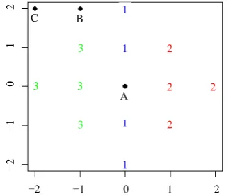
Considered set of training locations with indicated class labels is shown inFigure 1.

So we have small training sample sizes (i.e. n₁=n₂=n₃=4) and three different locations to be classified, furthermore we assume equal prior probabilities π =l 1 3, l=1, 2, 3.

[image:5.595.231.399.554.695.2]

Simulations were performed by geoR: a free and open-source package for geostatistical analysis included in statistical computing software R (http://www.r-project.org/). Each case was simulated 100 times (runs) and ACCR values are calculated by averaging ACCR over the runs. ACCR and CCR values are presented in Table 1. As might be expected ACCR values are lower than CCR. All values are increasing while range parame-ter is increasing. That means the stronger correlation gives betparame-ter accuracy of proposed classification procedures.

Figure 1. Locations of training sample: “1” are samples from population Ω1, “2” from Ω2, “3” from Ω3, A, B and C denotes

the locations of observation to be classified.

C B

A

3 3

3

3

1

1

1

1

2

2

2 2

−2 −1 0 1 2

−2

−1

0

1

Table 1. CCR and ACCR values.

θ CCR ACCR

A (0,0) B (−1,2) C (−2,2) A (0,0) B (−1,2) C (−2,2)

1 0.633777 0.634955 0.487689 0.544697 0.427956 0.404184

2 0.882716 0.839326 0.599707 0.636842 0.501045 0.483608

3 0.973217 0.948266 0.716064 0.725356 0.565855 0.480018

4 0.999777 0.955340 0.810298 0.773966 0.639186 0.553055

It’s seen inFigure 1, that the closest location to be classified is location A and the farthest is location C. CCR and ACCR _{are largest for location A and smallest for location C. It can be concluded that better accuracy gives} closer locations.

References

[1] McLachlan, G.J. (2004) Discriminant Analysis and Statistical Pattern Recognition. Wiley, New York.

[2] Dučinskas, K. (2009) Approximation of the Expected Error Rate in Classification of the Gaussian Random Field

Ob-servations. Statistics and Probability Letters, 79, 138-144. http://dx.doi.org/10.1016/j.spl.2008.07.042

[3] Batsidis, A. and Zografos, K. (2011) Errors of Misclassification in Discrimination of Dimensional Coherent Elliptic Random Field Observations. Statistica Neerlandica, 65, 446-461. http://dx.doi.org/10.1111/j.1467-9574.2011.00494.x

[4] Schervish, M.J. (1984) Linear Discrimination for Three Known Normal Populations. Journal of Statistical Planning and Inference, 10, 167-175. http://dx.doi.org/10.1016/0378-3758(84)90068-5

[5] Wu, T.F., Lin, C.J. and Weng, R.C. (2004) Probability Estimates for Multi-Class Classification by Pairwise Coupling.

Journal of Machine Learning Research, 5, 975-1005.

[6] Hirst, D. (1996) Error-Rate Estimation in Multiply-Group Linear Discriminant Analysis. Technometrics, 38, 389-399.

http://dx.doi.org/10.1080/00401706.1996.10484551

[7] Williams, C.K.I. and Barber, D. (1998) Bayesian Classification with Gaussian Processes. IEEE Translations on Pat-tern Analysis and Machine Intelligence, 20, 1342-1351. http://dx.doi.org/10.1109/34.735807

[8] Xu, T. and Wang, J. (2013) An Efficient Model-Free Estimation of Multiclass Conditional Probability. Journal of Sta-tistical Planning and Inference, 143, 2079-2088. http://dx.doi.org/10.1016/j.jspi.2013.08.008

[9] Schervish, M.J. (1981) Asymptotic Expansions for the Means and Variances of Error Rates. Biometrica, 68, 295-299.

http://dx.doi.org/10.1093/biomet/68.1.295

[10] Anderson, T.W. (2003) An Introduction to Multivariate Statistical Analysis. Wiley, New York.

[11] Šaltytė, J. and Dučinskas, K. (2002) Comparison of ML and OLS Estimators in Discriminant Analysis of Spatially

Correlated Observations. Informatica, 13, 297-238.

[12] Šaltytė-Benth, J. and Dučinskas, K. (2005) Linear Discriminant Analysis of Multivariate Spatial-Temporal Regressions.

Scandinavian Journal of Statistics, 32, 281-294. http://dx.doi.org/10.1111/j.1467-9469.2005.00421.x

[13] Dučinskas, K. (2011) Error Rates in Classification of Multivariate Gaussian Random Field Observation. Lithuanian

Mathematical Journal, 51, 477-485. http://dx.doi.org/10.1007/s10986-011-9142-4

[14] Dučinskas, K. and Dreižienė, L. (2011) Supervised Classification of the Scalar Gaussian Random Field Observations

under a Deterministic Spatial Sampling Design. Austrian Journal of Statistics, 40, 25-36.

[15] Dučinskas, K., Dreižienė, L. and Zikarienė, E. (2015) Multiclass Classification of the Scalar Gaussian Random Field Observation with Known Spatial Correlation Function. Statistics and Probability Letters, 98, 107-114.

http://dx.doi.org/10.1016/j.spl.2014.12.008

[16] Wackernagel, H. (2003) Multivariate Geostatistics: An Introduction with Applications. Springer-Verlag, Berlin.