Stability and Regularization Method for Inverse Initial Value Problem of Biparabolic Equation

(1)

How to cite this paper: Zhang, H.W. and Zhang, X.J. (2015) Stability and Regularization Method for Inverse Initial Value Problem of Biparabolic Equation. Open Access Library Journal, 2: e1542. http://dx.doi.org/10.4236/oalib.1101542

Stability and Regularization Method for

Inverse Initial Value Problem of Biparabolic

Equation

Hongwu Zhang, Xiaoju Zhang

School of Mathematics and Information Science, Beifang University of Nationalities, Yinchuan, China Email: [email protected]

Received 18 April 2015; accepted 6 May 2015; published 14 May 2015

This work is licensed under the Creative Commons Attribution International License (CC BY).

http://creativecommons.org/licenses/by/4.0/

Abstract

We consider an inverse initial value problem of the biparabolic equation; this problem is ill-posed and the regularization methods are needed to stabilize the numerical computations. This paper firstly establishes a conditional stability of Holder type, then uses a modified regularization me-thod to overcome its ill-posedness and gives the convergence estimate under an a-priori assump-tion for the exact soluassump-tion. Finally, a numerical example is presented to show that this method works well.

Keywords

Inverse Initial Value Problem, Biparabolic Equation, Conditional Stability, Regularization Method, Convergence Estimate

Subject Areas: Numerical Mathematics, Partial Differential Equation

1. Introduction

Let H be a complex separable Hilbert space endowed with the inner product ⋅ ⋅, and the norm ⋅ , and

( )

L H be the Banach algebra of bounded linear operators on H. Denote A D A:

( )

⊂H→H as a positive and self-adjoint operator with compact resolvent; λn

(

n≥1

)

is the real eigenvalues of A; Xn∈H is the corres-ponding orthonormal basis of eigenvectors, and λn satisfies

1 2 3

0 and lim n .

n

λ λ λ λ

→∞

< ≤ ≤ ≤ = ∞ (1)

(2)

OALibJ | DOI:10.4236/oalib.1101542 2 May 2015 | Volume 2 | e1542

( )

2

d

2 0, 0, ,

d

, t 0 0,

A u t u t Au t A u t t T

t

u T g u

 ₊  ₌ _′′ ₊ _′ ₊ ₌ _∈

_ _ 

 ₌ ₌



(2)

our purpose is to reconstruct the initial value f :=u

( )

0 from the final measured data gδ; here δ denotes the noisy level.

In past years, many authors have considered the inverse initial value problem of classical parabolic equation t

u = ∆a u with a>0 (see [1]-[4], etc.). However, it is well-known that the classical parabolic equation can not accurately describe the procedure of heat conduction [5] [6], so many models have been proposed to describe this procedure; among them the biparabolic model proposed in [7] can give a more adequate mathematical de-scription for the process of heat conduction than the classical case. Meanwhile we note that, for the biparabolic model, up to now the literatures devoted to it are relatively scarce, except for [7]-[9]. On other models, we can see [10]-[13], etc.

Problem (2) is ill-posed and the regularization techniques are required to stabilize numerical computations [14] [15]. In 2015, [9] considered this problem and proved a condition stability result of Hölder type, and then ap-plied the Kozlov-Maz’ya iteration method to deal with it; the corresponding convergence results have been giv-en, but unfortunately the condition stability result in [9] is not useful for the case of t=0. In this paper, we firstly establish a conditional stability of Hölder type, which is valid at the point t=0, then use a modified regu-larization method to overcome its ill-posedness and give the convergence estimate under an a-priori assumption for the exact solution. On the similar references for this regularization method, we can refer to [16]-[18], etc.

This paper is constructed as follows. In Section2, we establish the conditional stability of Hölder type for this problem, then use a modified regularization method to deal with it and derive the convergence estimate under an

a-priori assumption for the exact solution in Section 3. Numerical results are given in Section 4. Some conclu-sions are made in Section 5.

2. The Ill-Posedness and Conditional Stability Estimate

From [9], we know that the unique formal solution of problem (2) can be expressed as

( )

1

e , , .

1

n

T t n

n n n n

n n

t

u t g X g g X

T

λ λ

λ ∞

− =

 + 

= _ _ =

+

 

∑

(3)

It can be noticed that, for t∈

[

0,T

)

, 1 e( ) 1

n

T t n

n

t T

λ

λ λ

−

 + 

 ₊ 

  tends to infinity as n→ ∞, so in order to recovery

the stability of solution u t

( )

given by (3), the coefficient gn must decay rapidly. However, such a decay usually cannot occur for the measured data gδ, thus we have to use a regularization technique to restore nu-merical stability.

Note that,

( )

1

e

: 0 , , .

1

n

T

n n n n

n n

f u g X g g X

T λ λ ∞

=

= = =

+

∑

(4)

In general, under an additional a-priori bound assumption, a stability of the solution on the data can be ob-tained, this is called the conditional stability. Let p>0, E>0, here we assume the exact solution f :=u

( )

0

satisfy the a-priori condition

2

2 2

1

epT n , , ,

n n n n

n

f E f f X

λ λ ∞

=

≤ =

∑

(5)

now we give a conditional stability estimate of Hölder type for f :=u

( )

0 .

(3)

(

)

22 ₂

1, , ,

p

p _p

f ≤C λ p T E + g + ₍₆₎

where,

(

)

(

)

1 2 1 ₂ 1 1 1 , , 1 p p

C p T

T λ λ λ +     =_ _ +   .

Proof. Using (4), Hölder inequality, (5), we have

2 2 2

4 2

2 2

1 1 1

2 2 ₂ 2 2 2 ₂ 4 2 2 2 1 1 2

2 2 ₂

2

2 1

e e e

1 1 1

e

1

e 1

n n n

n

T T T p

p p

n n n n n

n n n n n n

p

p _p

p p

T p _p

p p

n n

n n n

p p

T p

p n

n n

f g X g g g

T T T

g g

T

g g

T

λ λ λ

λ

λ λ λ

λ λ ∞ ∞ ∞ + + = = = + ₊ + + ∞ ∞ + + = = + ₊ ∞ + =   = _ _ = = + + +     _ _    _ _  _   _ ≤  _ ₊ _  _ _ _ _             = = +    

∑

(

)

(

)

(

)

2

2 2 ₂

2

2 1

2 2

2 ₂ 2 ₂

2 2 2

2 2 2 1 1 2 2 2 ₂ 2 2 2 2 2 2 1

1 1 1 1

e e 1 1 e 1 e 1 1 1 1 e 1 1 n n n n n p p

T T p

p n

n n n

p _p _p

T p p

pT

p p

n p n n

n n n n n

p _p p pT p n n p p n g g T T

f g f g

T T f g T T λ λ λ λ λ λ λ λ

λ _λ _λ

λ

λ λ λ λ

+ ∞ + = + + ∞ ∞ + + = = + ∞ ₊ + =     + +             = = +   _ + _     _ _      ≤ _ _ ≤  ₊  _ _  ₊    

∑

2 4 2 ₂ 2 2_, p _p p p E g + + ₊  

from the above estimate, the conditional stability result (6) can be established.

3. Regularization Method and Convergence Estimate

Let the exact and noisy data g g, δ ∈H and satisfy

,

gδ −g ≤δ (7) where ⋅ denotes the H-norm. Based on the ill-posedness analysis in Section 2, we define the following mod-ified regularization solution

( )

1

1 e

: 0 , , .

1 1 e

n

T

n n n n

T

n n n

f u g X g g X

T

λ

δ δ δ δ

α α _λ _αλ λ

∞

=

= = =

+ +

∑

(8)

here, α >0 plays a role of the regularization parameter. In the following, we give the convergence estimate under an a-priori assumption for the exact solution f.

Theorem 3.1. Suppose that f given by (4) is the exact solution of problem (2) with the exact data g at t=0,

fαδ is the regularization solution defined by (8) with the measured data gδ. Let the measured data gδ sa-tisfy (7), and the a priori bound (5) is satisfied. If the regularization parameter is chosen as

2 2 , p E δ α _{=  }  +

  (9)

then we have the following convergence estimate

(

)

1

2 2 2 2 2 ln . p p p p

f_αδ f TE δ TE T δ E

−

+ +   ₊ 

− ≤ + _ _ __

 

  (10)

(4)

( )

1

, e xT h x x α − =

+ (11)

it is easy to verify that h x

( )

has a unique maximizer x0 as α <T such that

( )

0

(

)

₍

₎

ln

. 1 ln

T T

h x h x h

T T α α α   ≤ = _ _= +

  (12)

Note that

1 2

: .

f_αδ − f ≤ f_αδ −f_α + f_α−f = +I I (13)

We firstly give a estimate for I1. By (4), (5), (7), (8), using (12) and the fact

(

)

(

1 ln

)

T T

T α

α + α ≤ , we get

(

)

(

)

(

)

(

)

(

)

(

)

1 1 =1 1 =1 =1 1 1 1 e 1 1 1 e . 1 ln n n

n n n T

n n n

n n n T

n n

n n n n n n

n n

I f f g g X

T

g g X

T

T T

g g X g g X T

T

δ δ

α α λ

δ λ δ δ λ αλ λ αλ δ α α α α ∞ − = ∞ − ∞ ∞   = − = _ _ − + +     ≤_ _ − + +   ≤ − ≤ − ≤ +

∑

Below, we estimate I2. Using (4), (5), (8) with the exact data g, (12) and the inequality

(

)

(

1 ln

)

ln

(

)

T T

T

T α α

α + α ≤ , one can obtain that

(

)

(

)

(

)

2 2 2 2 1 2 1 2 2

2 2 2

1 2 2 2 2 2 1 1 1 e 1 e e 1 1 e 1 e e 1 e e . ln 1 ln n n n n n n n n n T n n T

n n n

T n

n n T

n n n

T pT n n T n _n pT n n n

I f f g X

T g X T g T T TE f T T λ α λ λ λ λ λ λ λ λ αλ αλ λ αλ α λ λ αλ α λ α α α ∞ − = ∞ − = ∞ − = ∞ =     = − =  ₊  −  +      − ≤  ₊  +       ≤ _ _ _ _ + + _ _       ≤ _ _ ≤_ _ + _ _  

∑

From the above estimates of I1, I2, and combining with (9), the triangle inequality (13), we can obtain the

convergence result (10).

4. Numerical Implementations

In this section, we use a numerical example to verify how this method works for the reconstruction of initial data

f. Consider the following forward problem

( )

(

)

( )

[ ]

( )

[ ]

( )

[ ]

2 2

2 , 0, 0,π , 0, ,

, 0 0, 0,π ,

, 0 sin sin 2 , 0,π ,

0, π, 0, 0, ,

t

u x t x t T

t x

u x x

u x x x x

u t u t t T

(5)

where _H =_L2

( )

_0,π

,

2

2 A

x

∂ = −

∂ with the domain

2 1

0 ( ) = (0, ) (0, )

D A H π



H π ⊂H , its eigenvalue and the eigenfunction are

λ

n =n2,

( )

2 sin π

n

X = nx , respectively.

By the method of separation of variables, it is easy to obtain that the solution of problem (14) can be ex-pressed as

( )

(

₂

)

2

( )

1

, n 1 e tn sin ,

n

u x t c tn nx

∞

− =

=

∑

+ (15)

where, π

(

( )

)

( )

0

2

sin sin 2 sin d π

n

c =

∫

x + x nx x. We take the exact data as

( )

(

)

(

₂

)

2

( )

1

, 1 e sin ,

m

Tn n

n

g x u x T c Tn − nx

=

= =

∑

+ (16)

the measured data is chosen as gδ

( )

x =g x

( )

+εrand size

(

( )

g

)

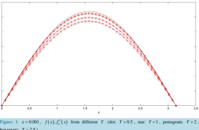
, where ε is the error level.

In the computational procedure, the exact and regularization solutions are computed by (4), (8), respectively. The regularization parameter α is chosen by (9) with p=1,E=1. For ε =0.001, the numerical results for

( )

, 0

[image:5.595.115.511.453.711.2]

f x =u x , f_αδ

( )

x =u_αδ

( )

x, 0 constructed from gδ =uδ

(

x T,

)

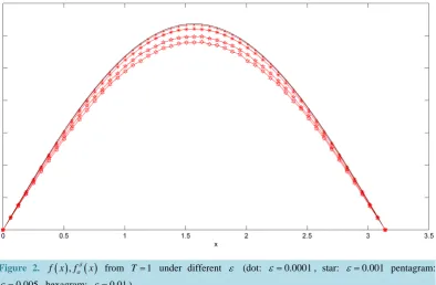
with T =0.5,1, 2, 2.5 are shown in

Figure 1. For ε=0.0001, 0.001, 0.005, 0.01, the numerical results for f x

( )

, f_αδ

( )

x constructed from T =1

are shown inFigure 2.

From Figure 1 and Figure 2, we can see that this method is effective and feasible. Figure 1 indicates that, with the increase of T, the construction effects become worse, this is because the information of final value data will become less when T becomes big. Figure 2 shows that the smaller ε is, the better the computed efficiency is, this is a normal phenomena in the inverse initial value problem of parabolic equation.

5. Conclusion

An inverse initial value problem of the biparabolic equation is investigated. We firstly establish a conditional stability of Hölder type for this problem, then use a modified regularization method to regularize it and derive

(6)

[image:6.595.116.511.86.344.2]

Figure 2. f x

( )

,f_αδ

( )

x from T=1 under different ε (dot: ε=0.0001, star: ε=0.001 pentagram: 0.005

ε= , hexagram: ε=0.01). the convergence estimate under an a-priori assumption for the exact solution. Numerical results show that this method is stable and feasible.

Acknowledgements

The authors thank for the careful work of the anonymous referee and the suggestions that improved the quality for our paper. This work is supported by the SRF (2014XYZ08), NFPBP (2014QZP02) of Beifang University of Nationalities, the SRP of Ningxia Higher School (NGY20140149) and SRP of State Ethnic Affairs Commission of China (14BFZ004).

References

[1] Cheng, J. and Liu, J.J. (2008) A Quasi Tikhonov Regularization for a Two-Dimensional Backward Heat Problem by a Fundamental Solution. Inverse Problems, 24, Article ID: 065012. http://dx.doi.org/10.1088/0266-5611/24/6/065012

[2] Feng, X.L., Qian, Z. and Fu, C.L. (2008) Numerical Approximation of Solution of Nonhomogeneous Backward Heat Conduction Problem in Bounded Region. Mathematics and Computers in Simulation, 79, 177-188.

http://dx.doi.org/10.1016/j.matcom.2007.11.005

[3] Liu, J.J. (2002) Numerical Solution of Forward and Backward Problem for 2-d Heat Conduction Equation. Journal of Computational and Applied Mathematics, 145, 459-482. http://dx.doi.org/10.1016/S0377-0427(01)00595-7

[4] Qian, Z., Fu, C.L. and Shi, R. (2007) A Modified Method for a Backward Heat Conduction Problem. Applied Mathe-matics and Computation, 185, 564-573. http://dx.doi.org/10.1016/j.amc.2006.07.055

[5] Fichera, G. (1992) Is The Fourier Theory of Heat Propagation Paradoxical? Rendiconti del Circolo Matematico di Pa-lermo, 41, 5-28.

[6] Joseph, L. and Preziosi, D.D. (1989) Heat Waves. Reviews of Modern Physics, 61, 41.

http://dx.doi.org/10.1103/revmodphys.61.41

[7] Fushchich, V.L., Galitsyn, A.S. and Polubinskii, A.S. (1990) A New Mathematical Model of Heat Conduction Processes. Ukrainian Mathematical Journal, 42, 210-216. http://dx.doi.org/10.1007/BF01071016

[8] Atakhadzhaev, M.A. and Egamberdiev, O.M. (1990) The Cauchy Problem for the Abstract Bicaloric Equation. Sibirs-kii MatematichesSibirs-kii Zhurnal, 31, 187-191.

(7)

[10] Ames, K.A. and Straughan, B. (1997) Non-Standard and Improperly Posed Problems. Academic Press, New York. [11] Carasso, A.S. (2010) Bochner Subordination, Logarithmic Diffusion Equations, and Blind Deconvolution of Hubble

Space Telescope Imagery and Other Scientifc Data. SIAM Journal on Imaging Sciences, 3, 954-980.

http://dx.doi.org/10.1137/090780225

[12] Payne, L.E. (2006) On a Proposed Model for Heat Conduction. IMA Journal of Applied Mathematics, 71, 590-599.

http://dx.doi.org/10.1093/imamat/hxh112

[13] Wang, L., Zhou, X. and Wei, X. (2008) Heat Conduction: Mathematical Models and Analytical Solutions. Springer- Verlag, Berlin.

[14] Engl, H.W., Hanke, M. and Neubauer, A. (1996) Regularization of Inverse Problems, Volume 375 of Mathematics and Its Applications. Kluwer Academic Publishers Group, Dordrecht.

[15] Kirsch, A. (1996)An Introduction to the Mathematical Theory of Inverse Problems. Volume 120 of Applied Mathe-matical Sciences. Springer-Verlag, New York. http://dx.doi.org/10.1007/978-1-4612-5338-9

[16] Ames, K.A., Clark, G.W., Epperson, J.F. and Oppenheimer, S.F. (1998) A Comparison of Regularizations for an Ill- Posed Problem. Mathematics of Computation, 67, 1451-1472. http://dx.doi.org/10.1090/S0025-5718-98-01014-X

[17] Clark, G.W. and Oppenheimer, S.F. (1994) Quasireversibility Methods for Non-Well-Posed Problems. Electronic Journal of Differential Equations, 1-9.