RAJKUMAR S
SCSEVIT University, Vellore
VIJAYARAJAN V
SCSEVIT University, Vellore
SHREY GUPTA
SCSEVIT University, Vellore
ANIL KUMAR
SCSE VIT University, VelloreABSTRACT
Image filter is the process of removing various types of noise from the images. The ensuant image is an information rich image than the original input image. The filtering finds its application in many fields from medical imagery, face detection, robot navigation, object detection, aircraft maintenance to image enhancement and image restoration. In the field of medical sciences the filter serves the purpose of image enhancement for efficient disease diagnosis, in aircraft maintenance for the purpose of detection of faults during takeoff, in case of face detection, object recognition and robot navigation used for object detection. This paper uses different quantitative metrics to analyze the result of different filtering techniques on an image. Initially, well known registered images from various aspects of science and nature are taken such as one image ct.jpg from medical sciences, two images Lighthouse.jpg, Penguins.jpg of natural scenery, two images of faces Koala.jpg, lena.jpg and a picture of naturally grown flowers Tulips.jpg are taken as input. Filtering techniques namely Median Filter (MF), Adaptive Filter (AF), New Adaptive Median Filer (NAMF), New Adaptive Spatial Filter (NASF), Edge Preserving Smooth Filter (EPSF) are applied on them. Further the filtered images are analyzed using five quantitative metrics such as Entropy (EN), Standard Deviation (SD), Peak Signal to Noise Ratio (PSNR), Mean Square Error (MSE), and Mean Absolute Error (MAE). From the experimental result and the corresponding metrics used we observed that the resultant image is more informative than the original source images.
General Terms
Image Enhancement, Salt and Pepper noise, Gaussian noise, Quantitative Analysis.
1. INTRODUCTION
In recent years, noises can occur from a number of resources. While capturing image from a sensor or transmitting image through a communication channel, image can get frequently contaminatedby several noises namely Salt- and- pepper noise, Gaussian noise etc. As a result of this, such corrupted images while being used for processing viz. image segmentation, object recognition, image fusion, and edge detection tend to provide unexpected results. Henceforth, before any processing, improving the quality of images play a vital role. The required improvement can be achieved using filtering techniques. Filtering techniques are classified into two types - linear filters and non-linear filters. Linear filters have a drawback that it fails to recover sharp pixel edge corrupted by noise. In addition,
impulse noise cannot be abridged adequately. Salt-and–pepper noise occurs when there is a fault or malfunction in the equipment capturing the picture or an error in the digitization process of the image or an error in storing the image to memory location. The performance of linear filters on Salt-and-pepper noise is unsatisfactory hence it cannot be used frequently [7, 8, 9].
Generally, Non-linear filter show better results than linear filter for removing such noise. To overcome these problems we have proposed the following non-linear filters namely Median Filter, Adaptive Filter, New Adaptive Median Filter, New Adaptive Spatial Filter, and Edge Preserving Smooth Filter. The main aim of these filters is to enhance the quality of image for richer image quality and better feature extraction.
Median filter (MF) utilizes median of the neighborhood of a pixel to smoothen the image [1].
The Adaptive Filter (AF) works in two stages, namely adaptive median-based filtering and statistics-based estimation. Adaptive median-based filter detects corrupted pixel in an image through estimation techniques and then statistical analysis corrects the corrupted pixel through the local neighborhood [2].
The New Adaptive Median Filter (NAMF) performs spatial processing to determine which pixels in an image have been affected by impulse noise i.e. this filter sets a threshold intensity value derived from a region of uniform amplitude. Thus it can detect impulse noise in a pixel when there is a large difference in the value of the pixel in consideration and threshold value set, replacing only noise corrupted pixels and not the noise-less ones. As a result reduces noise without blurring the image [3].
The New Adaptive Spatial Filter (NASF) uses discrete features of an image. It constructs a mask using the uniform regions of the image resulting in a better mask than the conventional spatial filter. It calculates a threshold value in an image and replaces the pixel data if and only if the difference between the highest pixel intensity and the lowest pixel intensity is less than the threshold value. The result is an enhanced image with reduced noise and better sharpness [4].
The Edge Preserving Smooth Filter (EPSF) reduces the noise and provides better edge preservation property [5].
The performances of the filtering techniques are evaluated based on the different quantitative metrics such as EN, SD, PSNR, MSE, and MAE.
The remaining sections of this paper organized as follows. In section II discusses the type of noise, section III system design briefly reviewed, section IV describes experimental
Analysis of Non-Linear Filtering Techniques based on
results and evaluates the performance of the proposed methods based on the quantitative metrics. Discussion and future work are summarized at the end.
2. TYPES OF NOISE
Normally, an image is affected by different types of noise. The most familiar types of noise are Impulse (Salt-and- Pepper) noise, Gaussian (Normal) noise, Uniform noise, Exponential noise, Gamma noise etc. In this paper, mainly Impulse (Salt-and-Pepper) noise is discussed. The following subsection briefly explains the noise detail.
2.1
Impulse Noise
The Probability Density Function (PDF) of Bipolar impulse noise is defined by [12]
otherwise
b
z
for
P
a
z
for
P
z
p
ba
0
)
(
(1)
If b > a, gray-level ‘a’ appears as a dark dot in the image. ‘b’ appears like a light dot in the image. If either
P
a orP
b is zero, the impulse noise called as unipolar noise. If neitherP
a orP
b is zero, and particularly if they are roughly equal, impulse noise values resemble Salt and Pepper granules randomly distributed over the image. The noise impulses can be either negative or positive. Negative impulses appear as black (Pepper)points in an image and positive impulses appear as white (Salt)noises. For an 8 bit image this means thata
0
(black) and255
[image:2.595.307.555.103.375.2]b
(white). The pictorial representation of impulse noise is shown in fig.1-2 [11].Fig 1: Probability Density Function of Impulse Noise
Fig 2: Representation of Salt-and-Pepper Noise
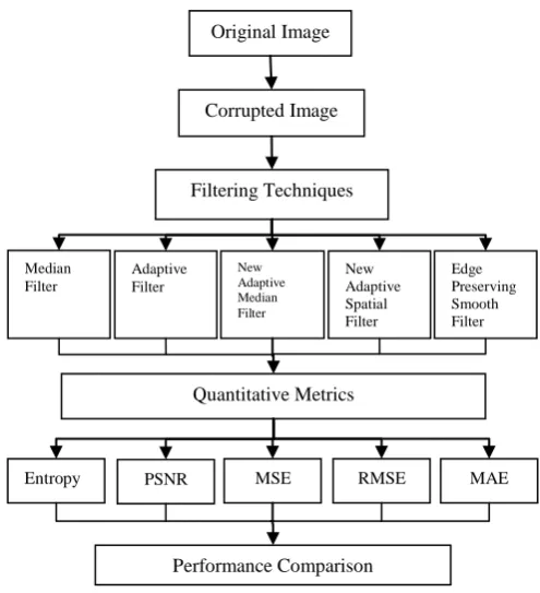
3. SYSTEM DESIGN
In this system initially registered gray scale image taken as input. Noise is applied to the input image and then the noisy image is filtered using different filtering techniques. Finally, the output filtered image is validated using quantitative measures.
The system design is shown in Fig. 3.
Fig 3: An overall view of system design
3.1
Median Filter
Median filter [1] is a non-linear filter that is often described in the spatial domain. It actually, removes Salt-Pepper noise from distorted image, but this image while filtering suffers the blurring effect. The median filter works by utilizing the median value of neighboring pixels. The calculation of median filter performs following task to find each pixel value in the processed image:
All pixels in the neighborhood of the pixel in the original image which are recognized by the mask are stored in the descending (or) ascending order.
The median of the stored value is computed and is chosen as the pixel value for the processed image.
Thus even the unaffected pixels are replaced by median value resulting in image distortion.
3.2 Adaptive Filter
The Adaptive Filter [2] works in two stages, namely adaptive median-based filtering and statistics-based estimation. In first stage, the adaptive median-based filter aims to detect corrupted pixel in order to replace its value with the noise-free median of local neighborhood. If it fails to obtain a noise-free pixel then statistics-based estimation is used to find the noise-free pixel. In second stage, statistical analysis corrects the corrupted pixel through the local neighborhood.
3.2.1 Adaptive Median-Based Filter:
Given an image A corrupted with salt-and-pepper noise, this algorithm first square windowW
2d1
i
,
j
with odd
2
d
1
*
2
d
1
dimensions centered on a corrupted Original ImageCorrupted Image
Filtering Techniques
Quantitative Metrics
Performance Comparison Adaptive
Filter
New Adaptive Median Filter
New Adaptive Spatial Filter
PSNR MSE RMSE MAE
Edge Preserving Smooth Filter Median
Filter
Entropy
b
a
b
p
p(z )
a
p
p(z ) p(z)
Impulse
[image:2.595.87.262.500.609.2]pixel
i
,
j
and calculates the median from the corresponding neighborhood. Formally, define the processing window as
i
j
A
i
x
j
y
W
2d1,
,
(2)Where x, y belongs to
d
....
0
,
1
....
d
.Initially, the algorithm start with d=1, and checks the median of the local neighborhood is noise-free or not. If a noise-free median is found, then the value of the corrupted pixel
i
,
j
is replaced with median value of local neighborhood. Suppose, the median value is noisy then the window size is expanded by incrementing the value of d by 1 and again algorithm checks for the noise-free median in local neighborhood. This process is repeated until a noise-free median is found or d reaches the pre-defined maximum window size
d
3
.If a noise-free median is found, the corrupted pixel is replaced by median value. If a noise-free median is not found, the corrupted pixel is subjected to further statistical analysis of the local neighborhood in order to estimate an accurate correction term.
3.2.2 Statistics-Based Estimation: Statistics-Based Estimation algorithm is used when the adaptive filter cannot find the noise-free median through the maximum size processing window. This can happen when the entire pixels in the image are corrupted. To solve this problem, Statistics-Based-Estimation checks the value of last processed pixel.
If the value of the last processed pixel is not 0 or 255, then the current pixel is considered as a noisy pixel. However in this case, basically using last processed pixel to replace the noise pixel may not be consistent for the property of local region. In order to perform well this method first checks the property of the region defined by window size is
9
*
9
. If a noise-free median is found in the neighborhood through the processing window then the noisy pixel is replaced with the last processed pixel value. Otherwise, the noisy pixel is replaced by the mode of the local neighborhood.3.3 New Adaptive Median Filter
This filter detects the impulse noise, for this it makes the assumption that a noisy pixel takes a gray value which is different from the neighboring pixels in the filtering window. Here, the difference of the median value of pixels in the filtering window and the current pixel value is compared with a threshold to make a decision about presence of the noise [3].
The New Adaptive Median Filter algorithm as follow as:
Step 1: Take a sub window of size
w
w
around the current pixel wherew
3
.Step 2: Move to step 1 if the difference between the maximum and minimum value of pixel is not above the threshold value under the window limit.
Step 3: Count all other pixel values excluding minimum and maximum values under the window limit.
Step 4: If the count value calculated in step 3 is greater than or equal to w than calculate the median value of pixels which are not the part of maximum and minimumvalue; else increase the size of the window by
w
w
2
and go to step 1.Step 5: Replace the current pixel by excluded median value if the current pixel is equal to maximum and minimum value; else leave it and move to next pixel and go to step 1.
3.4 New Adaptive Spatial Filter
This filter removes the Gaussian and impulse noise to produce a good quality image [4].
The New Adaptive Spatial Filter given below:
Consider an image f of size
M
N
and L gray levels. Step 1: Construct a matrix from the entire image so that pixel values
X
ij , of orderM
N
can be stored which is also called image resolution.Step 2: Add dummy rows or columns(whichever is suitable) if M & N are not the multiple of 3 to make them so.
Step 3: Make smaller matrixes of order
3
3
from the above obtained matrix.Step 4: Consider a
3
3
matrix
T
k and operate upon thisth
k
matrix,
1
k
M
N
/
9
as follows:Step 4.1: Identify the maximum
Max
k
and minimum
Min
k
from the entire given pixel values.Step 4.2: If
Max
k
Min
k is less than a threshold values (optimal value 200 obtained by trial and error) then calculate mean of the pixel values
X
ij over matrix
T
k as:
31 3
1
9
1
i
i j
j ij
X
x
(3)else consider the next matrix
T
k1 .Step 4.3: Construct a difference matrix
i
j
whose value is calculated as
i
j
X
ij
Step 4.4: Replace the value in the given 3×3 matrix with the pixel value corresponding to
min
i
j
.3.5 Edge Preserving Smoothing Filter
Sharpening and smoothing are two effects induced by this filter. The following steps calculate approximately sharpening and smoothing values [5].
Step 1: Plot a scattergram: A scattergram is plotted of the pixel of the gradient magnitude of the original image versus those of the gradient magnitude of the filtered image.
y
F
x
F
f
(4)
F
mag
f
F
x
2
F
y
2(5)
where
F
denotes the gradient magnitude of function
x
y
f
denotes the gradient vector of functionI
x
,
y
Step 2: Fit Lines: Fit liney
ax
b
used through the two sets to achieving density-independent factors in which edges are sharpened and flat regions are smoothed.
a
A,
b
A
arg
min
a,b
x,yAy
ax
b
(6)
a
B,
b
B
arg
min
a,b
x,yBy
ax
b
(7)where
a
A denotes the smoothing of the filtera
B indicate the sharpening of the filter
a
A
1
anda
B
1
are needed because values are cut at 1 is necessary.Step 3: Weight Slopes: The slopes found are weighted with the relative number of points used to specify the number of pixels actually used to estimate these values.
Smoothing
F
,
I
a
A1
1
A
A
B
(8)Sharpening
F
,
I
a
B1
1
B
A
B
(9)where
a
1A
1
a
AThe above two equation values can be considered to be an amplification factor of edges, and an attenuation factor of flat regions, respectively.
3.6 Quantitative Analysis on Filtered Image
The quantitative measurement (Performance Evaluation) is done on the filtered images using some objective and subjective quality measures. It helps better in assessing the information of images. This section explains the quantitative metrics used in the analysis of this system.3.6.1 Entopy(EN): Entropy can effectively reflect the amount of information in certain image. A larger value indicates that a better fusion result is obtained [6]
10
log
2L
i
P
Fi
P
Fi
EN
(10)where
P
F is the normalized histogram of the fused image to be evaluated, L is the maximum gray level for a pixel in the image. In our tests, L is set to 255.3.6.2Peak Signal to Noise Ratio (PSNR): PSNR is used to measure the quality of the image with respect to the original input image. It is defined as: [10]
10 1
0
2
,
,
/
1
p
i q
j
j
i
B
j
i
A
pq
MSE
(11)
PSNR
10
log
10
MAX
2MSE
(12)where MAX is the maximum value in an image. p, q are the height and weight of an image.
A
i
,
j
is the value of input image andB
i
,
j
is the value of filtered image.3.6.3
Standard Deviation (SD)
: Standard deviation defines the contrast information of an image. Image with more contrast has high value of standard deviation whereas images with low contrast have low values of standard deviation: [6]
N
i
x
ix
N
1 2/
1
(13)
Where x is defined as a summation
N
N
x
x
N
i
x
N
x
...
/
2
1 1
/
1
(14)3.6.4
Mean Square Error (MSE):
j
i
y
ijx
ijMN
MSE
,
2
1
(15)
where
y
ij denotes the corrupted image,x
ijdenotes the filtered image, MN total number of pixel in the image [2].3.6.5 Mean Absolute Error (MAE):
j
i
y
ijx
ijMN
MSE
,
1
(16)where
y
ij denotes the corrupted image,x
ijdenotes the filtered image, MN total number of pixel in the image [2].4.
EXPERIMENTAL
RESULTS
AND
PERFORMANCE
EVALUATION
[image:4.595.306.540.96.327.2]The experimental results of the filtering techniques are analyzed with six different types of gray scale images with jpg file extension. All images have the same size of
256
*
256
pixels, with 256-level gray scale. Input images are shown in Fig. 4.
Koala Lighthouse Penguins
Tulips CT Lena
[image:4.595.311.539.559.739.2]The above input images are corrupted with 10%, 20%, 30%, 40%, 50%, 60%, 70%, 80%, 90%, 100% with the fixed impulse noise. Some of the corrupted images with 40%, 70% and 90% impulse noise Shown in Fig. 5-7.
Fig 5: All the input images corrupted with noise level 40%
Fig 6: All the input images corrupted with noise level 70%
Fig 7: All the input images corrupted with noise level 90%
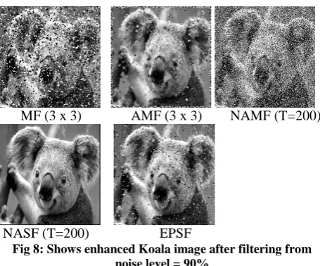
The resultant of the koala image derived from the 90% corrupted noise after applying different filters are shown in Fig. 8.
MF (3 x 3) AMF (3 x 3) NAMF (T=200)
[image:5.595.310.538.78.267.2]
NASF (T=200) EPSF
Fig 8: Shows enhanced Koala image after filtering from noise level = 90%
The resultant of the penguins image derived from the 90% corrupted noise after applying different filters are shown in Fig. 9.
MF (3 x 3) AMF (3 x 3) NAMF (T=200)
[image:5.595.55.287.121.280.2]NASF (T=200) EPSF
Fig 9: Shows enhanced Penguins image after filtering from noise level = 70%
The resultant of the CT image derived from the 40% corrupted noise after applying different filters are shown in Fig. 10.
MF (3 x 3) AMF (3 x 3) NAMF (T=200)
[image:5.595.311.533.541.727.2]NASF (T=200) EPSF
Fig 10: Shows enhanced Ct image after filtering from noise level = 40%
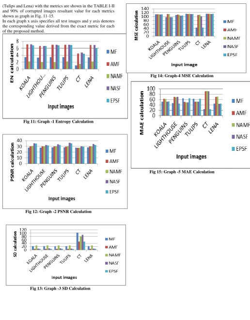
(Tulips and Lena) with the metrics are shown in the TABLE I-II and 90% of corrupted images resultant value for each metrics shown as graph in Fig. 11-15.
In each graph x axis specifies all test images and y axis denotes the corresponding value derived from the exact metric for each of the proposed method.
Fig 11: Graph -1 Entropy Calculation
[image:6.595.49.566.65.726.2]Fig 12: Graph -2 PSNR Calculation
Fig 13: Graph -3 SD Calculation
Fig 14: Graph-4 MSE Calculation
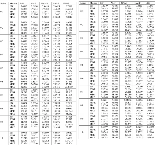
TABLE I: COMPARISON OF IMAGE FILTER ALGORITHM FOR TULIPS.JPG
TABLE II: COMPARISON OF IMAGE FILTER ALGORITHM FOR LENA.JPG
Noise Metrics MF AMF NAMF NASF EPSF
0.1 EN PSNR SD MSE MAE 7.6383 37.026 1.6990 12.775 7.0674 7.6690 39.214 1.6733 12.806 5.8722 7.4618 39.383 3.0941 12.822 5.8603 7.6623 45.642 1.7404 12.402 5.7662 6.7099 36.2253 1.1403 12.5731 6.8819 0.2 EN PSNR SD MSE MAE 7.6504 34.933 1.7085 25.437 14.020 7.6651 37.188 1.6733 25.820 11.617 7.0446 36.8707 5.7809 25.328 11.443 7.6075 44.378 2.2163 25.197 11.374 6.9213 37.514 1.1645 25.238 13.920 0.3 EN PSNR SD MSE MAE 7.6518 33.259 1.6818 38.663 21.367 7.6624 34.901 1.6902 38.393 17.334 6.5417 34.799 8.5845 38.220 17.319 7.5341 40.532 2.9557 38.120 17.302 6.9839 37.914 1.1762 38.195 20.965 0.4 EN PSNR SD MSE MAE 7.6154 32.358 1.9425 50.582 27.640 7.6547 33.663 1.7199 50.423 22.702 5.9901 32.823 11.346 50.337 22.815 7.4515 38.726 3.8168 50.249 22.210 6.9333 36.914 1.1811 50.740 28.105 0.5 EN PSNR SD MSE MAE 7.4275 31.068 3.2682 63.882 35.040 7.6421 32.998 1.7769 63.232 28.547 5.3260 32.522 14.346 63.240 28.786 7.3633 38.993 3.8168 62.552 27.774 6.7756 36.794 1.1904 64.652 28.105 0.6 EN PSNR SD MSE MAE 7.0164 29.061 5.9094 76.557 42.080 7.6333 31.601 1.8374 76.700 34.701 4.6251 31.5052 17.251 75.566 34.300 7.2717 38.012 4.7407 75.292 34.156 6.4685 37.619 1.1875 75.516 35.6727 0.7 EN PSNR SD MSE MAE 6.2695 28.785 9.9598 89.658 49.388 7.6156 30.773 1.9378 89.233 40.315 3.8816 30.687 20.115 88.363 39.976 7.1781 37.990 6.6919 88.197 39.216 6.7490 37.665 1.1606 88.869 41.556 0.8 EN PSNR SD MSE MAE 5.0464 29.266 15.526 101.98 56.376 7.5376 30.468 2.4224 101.51 45.889 3.0418 30.381 23.072 102.678 46.361 7.0833 37.562 7.7019 101.35 46.089 6.2001 37.387 1.0837 101.241 55.662 0.9 EN PSNR SD MSE MAE 3.4131 28.265 21.774 114.23 62.597 6.9460 29.382 6.2466 113.80 51.552 2.1156 29.928 25.988 114.879 51.9651 6.9880 36.452 8.7296 113.51 51.494 6.8625 35.587 4.3757 113.658 62.725 1.0 EN PSNR SD MSE MAE 0.9995 27.870 28.745 127.53 70.326 0.9999 29.471 28.737 126.41 57.210 0.9999 29.543 28.737 127.898 57.943 6.8927 35.984 9.7732 126.13 57.100 6.0712 35.872 8.6900 127.215 69.906
Noise Metrics MF AMF NAMF NASF EPSF
[image:7.595.39.573.105.606.2]5. CONCLUSIONS
In this paper, five different filtering techniques with quantitative metrics (performance evaluation) are analyzed with six different types of images contaminated with salt-and-pepper noise of varying densities such as CT, Koala, Penguins, Tulips, Lighthouse and Lena. The result shows that NASF technique outperforms than remaining filter techniques from the visual perspective which is also verified with the quantitative metrics. From Table I, II and figure 11, 12, 13, 14, 15 observed that higher values of EN and PSNR provides enhanced information for NASF, lower values of SD ensure that contrast information for EPSF, a lower values of MSE that is a better reconstruction of original image from the noisy image, similarly MAE is much better predictor of image quality with a lower value resulting in a good image. These filtering techniques lead to many computational merits in reality which includes: efficient retrieval, reorganization objects easily, and can able to diagnosis disease.
In future work, we are interested to discover the effective other filter techniques for different types of noisy images and improve the performance of the system.
6. REFERENCES
[1] Sanjay Singh , Chauhan R.P.S, Devendra Singh “Comparative Study of Image Enhancement using Median and High Pass Filter-ing Methods”, Journal of Information and Operations Management, vol. 3,pp.96-98, 2012.
[2] Muhammad Mizanur Rahman, Faisal Ahmed, Mohammed Imrul JubairSyed Ashfaqueuddin Priom, Imtiaz Masud Ziko “An Enhanced Non-Linear Adaptive Filteing Technique for Removing High Density Salt-and-Pepper Noise”, International Journal of Computer Applications, vol.38, no.11, pp.7-12, January 2012.
[3] Punyaban Patel, Banshidhar Majhi, Abhishek Tripathi, C.R. Tripathy, “A New Adaptive Median Filtering
Technique for Removal of Impulse Noise from Images”, ICCCS’11, pp.462-467, February 2011.
[4] Amiya Halder, Sandeep Shekhar, Shashi Kant, Musheer Ahmed Mubarki, Anand Pandey “A New Efficient Adaptive Spatial Filter for Image Enhancement”, Second International Conference on Computer Engineering and Applications, pp.244-246, 2010.
[5] Shawn Chen, Tian-Yuan Shih, “On the evaluation of edge preserving smoothing filter, In Proceeding Geoinformatics, p.p C43, 2002.
[6] S.Rajkumar, S.Kavitha, “ Redundancy Discrete Wavelet Transform and Contourlet Transform for Multimodality Medical Image Fusion with fQuantitative Analysis”, 3rd International Conference on Emerging Trends in Engineering and Technology, November 2010.
[7] Shuyue Chen, Yun Qiu, Jun Feng, “A Nonlinear Filter Based on Row and Column Operation for Positive Impulsive Noise Reduction”, Asia-Pacific Conference on Information Processing, pp.44-46, 2009.
[8] Zhou Dengwen and Shen Xiaoliu, “Image Denoising Using Weighted Averaging”, International Conference on Communications and Mobile Computing, pp.400-403, 2009.
[9] Banshidhar Majhi,” Soft Computing Techniques for Image Restoration”, PhD Thesis, Sambalpur University, 2003.
[10]Krishan Kant Lavania, Shivali, Rajiv Kumar, “ Image Enhancement using Filtering Techniques”, International Journal of Computer Science and Engineering, vol.4, pp.14-20, January 2012.
[11]A.K.Jain, “Fundamentals of digital image processing”, Prentice-Hall of India,1989