Copulas for finance

Copulas for finance

Bouye, Eric and Durlleman, Valdo and Nikeghbali, Ashkan

and Riboulet, Gaël and Roncalli, Thierry

Crédit Lyonnais

7 March 2000

Online at

https://mpra.ub.uni-muenchen.de/37359/

A Reading Guide and Some Applications

Eric Bouy´

e

Financial Econometrics Research Centre

City University Business School

London

Valdo Durrleman

Ashkan Nikeghbali

Ga¨

el Riboulet

Thierry Roncalli

Groupe de Recherche Op´

erationnelle

Cr´

edit Lyonnais

Paris

First version: March 7, 2000

This version: July 23, 2000

Abstract

Copulas are a general tool to construct multivariate distributions and to investigate dependence structure between random variables. However, the concept of copula is not popular in Finance. In this paper, we show that copulas can be extensively used to solve many financial problems.

Contents

1 Introduction 3

2 Copulas, multivariate distributions and dependence 3

2.1 Some definitions and properties . . . 3

2.2 Dependence . . . 7

2.2.1 Measure of concordance . . . 7

2.2.2 Measure of dependence . . . 9

2.2.3 Other dependence concepts . . . 11

2.3 A summary of different copula functions . . . 13

2.3.1 Copulas related to elliptical distributions . . . 13

2.3.2 Archimedean copulas . . . 17

2.3.3 Extreme value copulas . . . 18

3 Statistical inference of copulas 20 3.1 Simulation techniques . . . 20

3.2 Non-parametric estimation . . . 21

3.2.1 Empirical copulas . . . 21

3.2.2 Identification of an Archimedean copula . . . 22

3.3 Parametric estimation . . . 23

3.3.1 Maximum likelihood estimation . . . 24

3.3.2 Method of moments . . . 27

4 Financial Applications 28 4.1 Credit scoring . . . 28

4.1.1 Theoretical background on scoring functions: a copula interpretation . . . 28

4.1.2 Statistical methods with copulas . . . 28

4.2 Asset returns modelling . . . 28

4.2.1 Portfolio aggregation . . . 29

4.2.2 Time series modelling . . . 29

4.2.3 Markov processes . . . 29

4.2.3.1 The_∗product and Markov processes . . . 29

4.2.3.2 An investigation of the Brownian copula . . . 30

4.2.3.3 Understanding the temporal dependence structure of diffusion processes . . . 33

4.3 Risk measurement . . . 37

4.3.1 Loss aggregation and Value-at-Risk analysis . . . 40

4.3.1.1 The discrete case . . . 40

4.3.1.2 The continuous case . . . 40

4.3.2 Multivariate extreme values and market risk . . . 45

4.3.2.1 Topics on extreme value theory . . . 45

4.3.2.2 Estimation methods . . . 50

4.3.2.3 Applications . . . 53

4.3.3 Survival copulas and credit risk . . . 62

4.3.4 Correlated frequencies and operational risk . . . 62

1

Introduction

The problem of modelling asset returns is one of the most important issue in Finance. People generally use gaussian processes because of their tractable properties for computation. However, it is well known that asset returns are fat-tailed. Gaussian assumption is also the key point to understand the modern portfolio theory. Usually, efficient portfolios are given by the traditional mean-variance optimisation program (Markowitz [1987]):

sup

α α

⊤_{µ u.c.}

 



α⊤_Σα≤s

α⊤_{1= 1}

α_≥0

(1)

with µ the expected return vector of the N asset returns and Σ the corresponding covariance matrix. The problem of the investor is also to maximize the expected return for a given variance. In the portfolio analysis framework,the variance corresponds to the risk measure, but it implies that the world is gaussian

(Schmock_andStraumann_[1999],Tasche_{[1999]). The research on value-at-risk (and capital allocation) has} then considerably modified the concept of risk measure (Artzner_, Delbaen_,Eber _andHeath_{[1997,1999]).}

Capital allocation within a bank is getting more and more important as the regulatory requirements are moving towards economic-based measures of risk (see the reports [1] and [3]). Banks are urged to build sound internal measures of credit and market risks for all their activities (and certainly for operational risk in a near future). Internal models for credit, market and operational risks are fundamental for bank capital allocation in abottom-up approach. Internal models generally face an important problem which is the modelling of joint distributions of different risks.

These two difficulties (gaussian assumption and joint distribution modelling) can be treated as a problem of

copulas. A copula is a function that links univariate marginals to their multivariate distribution. Before 1999, copulas have not been used in finance. There have been recently some interesting papers on this subject (see for example the article of Embrechts_,McNeil _and Straumann_{[1999]). Moreover, copulas are more often} cited in the financial litterature. Li_{[1999] studies the problem of default correlation in credit risk models, and} shows that “the current CreditMetrics approach to default correlation through asset correlation is equivalent to using a normal copula function”. In the Risk special report of November 1999 on Operational Risk,Ceske_and Hern´andez _{[1999] explain that copulas may be used in conjunction with Monte Carlo methods to aggregate} correlated losses.

The aim of the paper is to show that copulas could be extensively used in finance. The paper is organized as follows. In section two, we present copula functions and some related fields, in particular the concept of dependence. We then consider the problem of statistical inference of copulas in section three. We focus on the estimation problem. In section four, we provide applications of copulas to finance. Section five concludes and suggests directions for further research.

2

Copulas, multivariate distributions and dependence

2.1

Some definitions and properties

Definition 1 (Nelsen (1998), page 39) 1_{A N-dimensional copula is a function C with the following}

prop-erties2_:

1_{The original definition given by}Sklar_{[1959] is (in french)}

Nous appelerons copule (`andimensions) tout fonctionCcontinue et non-d´ecroissante — au sens employ´e pour une fonction de r´epartition `andimensions — d´efinie sur le produit Cart´esien denintervalles ferm´es [0,1] et satisfaisant aux conditionsC(0, . . . ,0) = 0 etC(1, . . . ,1, u,1, . . . ,1) =u.

1. DomC=IN = [0,1]N;

2. C is grounded andN-increasing3_;

3. C has margins Cn which satisfy Cn(u) =C(1, . . . ,1, u,1, . . . ,1) =ufor alluinI.

A copula corresponds also to a function with particular properties. In particular, because of the second and third properties, it follows that ImC =I, and so C is a multivariate uniform distribution. Moreover, it is obvious that ifF1, . . . ,FN are univariate distribution functions,C(F1(x1), . . . ,Fn(xn), . . . ,FN(xN)) is a multivariate

distribution function with margins F1, . . . ,FN because un = Fn(xn) is a uniform random variable. Copula

functions are then an adapted tool to construct multivariate distributions.

Theorem 2 (Sklar’s theorem) Let F be an N-dimensional distribution function with continuous margins F1, . . . ,FN. ThenF has a unique copula representation:

F(x1, . . . , xn, . . . , xN) =C(F1(x1), . . . ,Fn(xn), . . . ,FN(xN)) (3)

The theorem of Sklar_{[1959] is very important, because it provides a way to analyse the dependence structure} of multivariate distributions without studying marginal distributions. For example, if we consider the Gumbel’s bivariate logistic distributionF(x1, x2) = (1 +e−x1+e−x2)−

1

defined onR2_{. We could show that the marginal} distributions areF1(x1)≡RRF(x1, x2)dx2 = (1 +e−

x1₎−1 _{and F}

2(x2) = (1 +e−x2)− 1

. The copula function corresponds to

C(u1, u2) = F¡F−11(u1),F−21(u2)¢

= u1u2

u1+u2−u1u2

(4)

However, asFrees_and Valdez_{[1997] note,it is not always obvious to identify the copula. Indeed, for many} financial applications, the problem is not to use a given multivariate distribution but consists in finding a conve-nient distribution to describe some stylized facts, for example the relationships between different asset returns. In most applications, the distribution is assumed to be a multivariate gaussian or a log-normal distribution for tractable calculus, even if the gaussian assumption may not be appropriate. Copulas are also a powerful tool for finance, because the modelling problem can be splitted into two steps:

• the first step deals with the identification of the marginal distributions;

• and the second step consists in defining the appropriate copula in order to represent the dependence structure in a good manner.

In order to illustrate this point, we consider the example of assets returns. We use the database of the London Metal Exchange4 _{and we consider the spot prices of the commodities Aluminium Alloy (AL), Copper (CU),}

Nickel (NI), Lead (PB) and the 15 months forward prices of Aluminium Alloy (AL-15), dating back to January 1988. We assume that the distribution of these asset returns is gaussian. In this case, the corresponding ML estimate of the correlation matrix is given by the table 1.

Figure 1 represents the scatterplot of the returns AL and CU, the corresponding gaussian 2-dimensional covariance ellipse for confidence levels 95% and 99%, and the implied probability density function. Figure 2 contains the projection of the hyper-ellipse of dimension 5 for the asset returns. The gaussian assumption is

3_{CinN-increasing if theC-volume of allN-boxes whose vertices lie inI}N _{are positive, or equivalently if we have}

2

X

i1=1

· · ·

2

X

iN=1

(−1)i1+···+iN_{C u}

1,i1, . . . , uN,iN

≥0 (2)

for all u1,1, . . . , uN,1and u1,2, . . . , uN,2inIN withun,1≤un,2.

4_{In order to help the reader to reproduce the results, we use the public database available on the web site of the LME:}

AL AL-15 CU NI PB

AL 1.00 0.82 0.44 0.36 0.33

AL-15 1.00 0.39 0.34 0.30

CU 1.00 0.37 0.31

NI 1.00 0.31

PB 1.00

Table 1: Correlation matrixρof the LME data

generally hard to verify becauserare events occur more often than planned (see the outliers of the covariance ellipse for a 99.99% confidence level on the density function in figure 1). Figure 3 is a QQ-plot of the theoret-ical confidence level versus the empirtheoret-ical confidence level of the error ellipse. It is obvious that the gaussian hypothesis fails.

Figure 1: Gaussian assumption (I)

In the next paragraph, we will present the concept of dependence and how it is linked to copulas. Now, we present several properties that are necessary to understand how copulas work and why they are an attractive tool. One of the main property concernsconcordance ordering, defined as follows:

Definition 3 (Nelsen (1998), page 34) We say that the copulaC1is smaller than the copulaC2 (orC2 is

larger thanC1), and writeC1≺C2 (orC1≻C2) if

Figure 2: Gaussian assumption (II)

Two specific copulas play an important role5, the lower and upper Fr´echet boundsC− andC+:

C−(u1, . . . , un, . . . , uN) = max

à _N X

n=1

un−N+ 1,0

!

C+(u1, . . . , un, . . . , uN) = min (u1, . . . , un, . . . , uN) (6)

We could show that the following order holds for any copulaC:

C− ≺C≺C+ (7)

The concept of concordance ordering can be easily illustrated with the example of the bivariate gaussian copula

C(u1, u2;ρ) = Φρ¡Φ−1(u1),Φ−1(u2)¢(Joe [1997], page 140). For this family, we have

C− _=C

ρ=−1≺Cρ<0≺Cρ=0=C⊥≺Cρ>0≺Cρ=1=C+ (8)

withC⊥ _{theproduct copula}6_{. We have represented this copula and the Fr´echet copulas in the figure 4. Level}

curves©

(u1, u2)∈I2|C(u1, u2) =Cªcan be used to understand the concordance ordering concept. Considering

formula (7), the level curves lie in the area delimited by the lower and upper Fr´echet bounds. In figure 5, we consider the Frank copula7_{. We clearly see that the Frank copula is positively ordered by the parameter α.}

Moreover, we remark that the lower Fr´echet, product and upper Fr´echet copulas are special cases of the Frank copula whenαtends respectively to_−∞, 0 and +_∞. This property is interesting because a parametric family could cover the entire range of dependence in this case.

Remark 4 The density c associated to the copula is given by

c(u1, . . . , un, . . . , uN) =

∂C(u1, . . . , un, . . . , uN)

∂ u1· · ·∂ un· · ·∂ uN

(11)

To obtain the densityf of the N-dimensional distribution F, we use the following relationship:

f(x1, . . . , xn, . . . , xN) =c(F1(x1), . . . ,Fn(xn), . . . ,FN(xN)) N

Y

n=1

fn(xn) (12)

wherefn is the density of the marginFn.

2.2

Dependence

2.2.1 Measure of concordance

Definition 5 (Nelsen (1998), page 136) A numeric measureκof association between two continuous ran-dom variablesX1 andX2 whose copula is Cis a measure of concordance if it satifies the following properties:

1. κis defined for every pair X1,X2 of continuous random variables;

2. ₋1 =κX,−X≤κC≤κX,X = 1;

5_C−_{is not a copula ifN >2, but we use this notation for convenience.}

6_{The product copula is defined as follows:}

C⊥=

N

Y

n=1

un (9)

7_{The copula is defined by}

C(u1, u2) =

1

αln

1 +(exp (αu1)−1) (exp (αu2)−1) (exp (α)−1)

(10)

Figure 4: Lower Fr´echet, product and upper Fr´echet copulas

3. κX1,X2 =κX2,X1;

4. if X1 andX2 are independent, thenκX1,X2 =κC⊥ = 0;

5. κ−X1,X2 =κX1,−X2=−κX1,X2;

6. if C1≺C2, thenκC1≤κC2;

7. if {(X1,n, X2,n)} is a sequence of continuous random variables with copulas Cn, and if {Cn} converges

pointwise to C, thenlimn→∞κCn=κC.

Remark 6 Another important property of κ comes from the fact the copula function of random variables

(X1, . . . , Xn, . . . , XN)is invariant under strictly increasing transformations:

CX1,...,Xn,...,XN =Ch1(X1),...,hn(Xn),...,hN(XN) if ∂xhn(x)>0 (13) Among all the measures of concordance, three famous measures play an important role in non-parametric statistics: the Kendall’s tau, the Spearman’s rho and the Gini indice. They could all be written with copulas, and we have (Schweitzer_and Wolff_[1981])

τ = 4

Z Z

I2

C(u1, u2) dC(u1, u2)−1 (14)

̺ = 12

Z Z

I2

u1u2dC(u1, u2)−3 (15)

γ = 2

Z Z

I2

(_|u1+u2−1| − |u1−u2|) dC(u1, u2) (16)

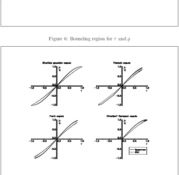
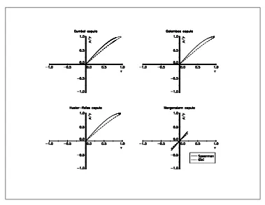
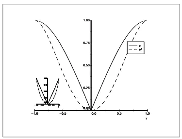
Nelsen_{[1998] presents some relationships between the measuresτand̺, that can be summarised by a bounding} region (see figure 6). In Figure 7 and 8, we have plotted the links betweenτ, ̺and γ for different copulas8_.

We note that the relationships are similar. However, some copulas do not cover the entire range [₋1,1] of the possible values for concordance measures. For example, Kimeldorf-Sampson, Gumbel, Galambos and H¨ usler-Reiss copulas do not allow negative dependence.

2.2.2 Measure of dependence

Definition 7 (Nelsen (1998), page 170) A numeric measureδ of association between two continuous ran-dom variablesX1 andX2 whose copula is Cis a measure of dependence if it satifies the following properties:

1. δ is defined for every pair X1,X2 of continuous random variables;

2. 0 =δC⊥ ≤δC≤δC+= 1;

3. δX1,X2 =δX2,X1;

4. δX1,X2 =δC⊥ = 0if and only ifX1 andX2 are independent;

5. δX1,X2 =δC+= 1 if and only ifeach ofX1 andX2 is almost surely a strictly monotone function of the other;

8_{If analytical expressions are not available, they are computed with the following equivalent formulas}

τ = 1−4

Z Z

I2

∂u1C(u1, u2)∂u2C(u1, u2) du1du2 (17)

̺ = 12

Z Z

I2C(u1, u2) du1du2−3 (18)

γ = 4

Z

I

(C(u, u) +C(u,1−u)−u) du (19)

Figure 6: Bounding region forτ and̺

Figure 8: Relationships betweenτ,̺andγfor some copula functions (II)

6. if h1 andh2 are almost surely strictly monotone functions on ImX1 andImX2 respectively, then

δh1(X1),h2(X2)=δX1,X2

7. if {(X1,n, X2,n)} is a sequence of continuous random variables with copulas Cn, and if {Cn} converges

pointwise to C, thenlimn→∞δCn=δC.

Schweitzer_andWolff_{[1981] provide different measures which satisfy these properties:}

σ = 12

Z Z

I2

¯

¯C(u1, u2)−C⊥(u1, u2)

¯

¯du1du2 (20)

Φ2 _{= 90}Z Z

I2

¯

¯C(u1, u2)−C⊥(u1, u2)

¯ ¯

2

du1du2 (21)

where σ is known as the Schweitzer or Wolff’s σ measure of dependence, while Φ2 _{is the dependence index}

introduced by Hoeffding.

2.2.3 Other dependence concepts

There are many other dependence concepts, that are useful for financial applications. For example,X1 andX2

are said to be positive quadrant dependent (PQD) if

Pr{X1> x1, X2> x2} ≥Pr{X1> x1}Pr{X2> x2} (22)

Suppose thatX1 andX2are random variables standing for two financial losses.The probability of simultaneous

large losses is greater for dependent variables than for independent ones. In term of copulas, relation (22) is equivalent to

Figure 9: Dependence measures for the Gaussian copula

The notion of tail dependence is more interesting. Joe_{[1997] gives the following definition:}

Definition 8 If a bivariate copula C is such that9

lim

u→1

¯ C(u, u)

1₋u =λ (27)

exists, then Chas upper tail dependence forλ∈(0,1]and no upper tail dependence for λ= 0.

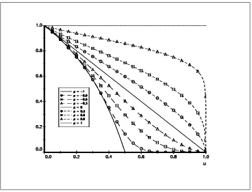
The measureλ is extensively used in extreme value theory. It is the probability that one variable is extreme given that the other is extreme. Letλ(u) = Pr_{U1> u|U2> u}=

¯ C(u,u)

1−u . λ(u) can be viewed as a

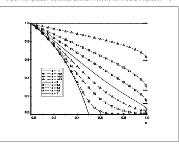
“quantile-dependent measure of dependence” (Coles_,Currie_andTawn_{[1999]). Figure 10 represents the values ofλ(u)} for the gaussian copula. We see that extremes are asymptotically independent for ρ₆= 1, i.e λ= 0 forρ <1. Embrechts_, McNeil _and Straumann _{[1999] remarked that the Student’s copula provides an interesting} contrast with the gaussian copula. We have reported the values ofλ(u) for the Student’s copula with one and

9_C¯ _{is the joint survival function, that is}

¯

C(u1, u2) = 1−u1−u2+C(u1, u2) (24)

Note that it is related to the survival copulaCˇ ˇ

C(u1, u2) =u1+u2−1 +C(1−u1,1−u2) (25)

in the following way

¯

five degrees of freedom10respectively. In this case, extremes are asymptotically dependent forρ6= 1. Of course, the strength of this dependence decreases as the degrees of freedom increase, and the limit behaviour asν tends to infinity corresponds to the case of the gaussian copula.

Figure 10: Quantile-dependent measureλ(u) for the gaussian copula

2.3

A summary of different copula functions

2.3.1 Copulas related to elliptical distributions

Elliptical distributions have density of the form f¡

x⊤_x¢

, and so density contours are ellipsoids. They play an important role in finance. In figure 13, we have plotted the contours of bivariate density for the gaussian copula and differents marginal distributions. We verify that the gaussian copula with two gaussian marginals correspond to the bivariate gaussian distribution, and that the contours are ellipsoids. Building multivariate distributions with copulas becomes very easy. For example, figure 13 contains two other bivariate densities with different margins. In figure 14, margins are the same, but we use a copula of the Frank family. For each figure, we have choosen the copula parameter in order to have the same Kendall’s tau (τ = 0.5). The dependence structure of the four bivariate distributions can be compared.

Definition 9 (multivariate gaussian copula — MVN_{) Let ρbe a symmetric, positive definite matrix with} diagρ=1andΦρ the standardized multivariate normal distribution with correlation matrixρ. The multivariate

gaussian copula is then defined as follows:

C(u1, . . . , un, . . . , uN;ρ) =Φρ¡Φ−1(u1), . . . ,Φ−1(un), . . . ,Φ−1(uN)¢ (28)

Figure 11: Quantile-dependent measure λ(u) for the Student’s copula (ν= 1

Figure 13: Contours of density for Gaussian copula

The corresponding density is11

c(u1, . . . , un, . . . , uN;ρ) =

1

|ρ_|12

exp µ

−1₂ς⊤¡

ρ−1−I¢ ς

¶

(31)

withςn=Φ−1(un).

Even if theMVNcopula has not been extensively used in papers related to this topic, it permits tractable calculus like theMVNdistribution. Let us consider the computation of conditional density. LetU=£

U⊤

1,U⊤2

¤⊤ denote a vector of uniform variates. In partitioned form, we have

ρ= ·

ρ11 ρ12

ρ22

¸

(32)

We could also show that the conditional density ofU2given values ofU1 is

(33)

c(U2|U1;ρ) = 1

¯

¯ρ22−ρ⊤12ρ− 1 11ρ12

¯ ¯ 1 2 exp µ

−1₂ς³£

ρ22−ρ⊤12ρ−111ρ12¤− 1

−I´_ς

¶

(34)

with ς =Φ−1_(U

2)−ρ⊤12ρ11−1Φ−1(U1). Using this formula and if the margins are specified, we could perform

quantile regressions or calculate other interesting values like expected values.

Definition 10 (multivariate Student’s copula — MVT_{) Let ρ be a symmetric, positive definite matrix}

with diagρ =1and Tρ,ν the standardized multivariate Student’s distribution12 with ν degrees of freedom and

correlation matrixρ. The multivariate Student’s copula is then defined as follows:

C(u1, . . . , un, . . . , uN;ρ, ν) =Tρ,ν¡t−ν1(u1), . . . , t−ν1(un), . . . , t−ν1(uN)¢ (36)

witht−1

ν the inverse of the univariate Student’s distribution. The corresponding density is13

c(u1, . . . , un, . . . , uN;ρ) =|ρ|−

1 2 Γ

¡ν+N

2

¢ £ Γ¡ν

2

¢¤N £

Γ¡ν+1 2

¢¤N Γ¡ν

2

¢ ¡

1 + 1_νς⊤_ρ−1_ς¢−ν+2N

N

Y

n=1

³ 1 +ς2n

ν

´−ν+12

(37)

withςn=t−ν1(un).

Remark 11 Probability density function ofMVNandMVTcopulas are easy to compute. For cumulative density functions, the problem becomes harder. In this paper, we use theGAUSSprocedurecdfmvnbased on the algorithm developed by Ford _{and the FORTRANsubroutine mvtdstwritten by} Genz_and Bretz_{[1999a,1999b].}

11_{We have for the Multinormal distribution}

1 (2π)N2 _|ρ|12

exp

−1

2x

⊤_ρ−1_x

=c(Φ(x1), . . . ,Φn(xn), . . . ,ΦN(xN)) N

Y

n=1

1

√

2πexp

−1 2x 2 n ! (29)

We deduce also

c(u1, . . . , un, . . . , uN) = 1

(2π)N2|ρ|12

exp −12ς⊤ρ−1ς

1

(2π)N2

exp −12ς⊤ς

(30)

12_{We have}

Tρ,ν(x1, . . . , xN) =

Z x1

−∞· · ·

ZxN −∞

Γν+₂N|ρ_|−12

Γ ν

2

(νπ)N2

1 +1

νx ⊤_ρ−1_x

−ν+₂N

dx (35)

There are few works that focus onelliptical copulas. However, they could be very attractive. Song _[2000] gives a multivariate extension of dispersion models with the Gaussian copula. Jorgensen _{[1997] defines a} dispersion modelY _{∼ DM}¡

µ, σ2¢

with the following probability density form

f¡

y;µ, σ2¢ =a¡

y;σ2¢ exp

µ

−₂1_σ2d(y;µ)

¶

(38)

µand σ2 are called theposition anddispersion parameters. dis theunit deviance withd(y;µ)≥0 satisfying

d(y;y) = 0. If a¡ y;σ2¢

takes the form a1(y)a2¡σ2¢, the model is a proper dispersion model PDM (e.g.

Simplex, Leipnik or von Mises distribution). Withd(y;µ) =yd1(µ) +d2(y) +d3(µ), we obtain an exponential

dispersion model _EDM (e.g. Gaussian, exponential, Gamma, Poisson, negative binomial, binomial or inverse Gaussian distributions). Jorgensen_andLauritzen_{[1998] propose a multivariate extension of the dispersion} model defined by the following probability density form

f(y;µ,Σ) =a(y; Σ) exp µ

−1₂trnΣ−1t(y;µ)t(y;µ)⊤o ¶

(39)

As noted by Song, this construction is not natural, becausetheir models are not marginally closed in the sense that the marginal distributions may not be in the given distribution class. Song _{[2000] proposes to define the} multivariate dispersion modelY_{∼ MDM}¡

µ, σ2_{, ρ}¢ as

f¡

y;µ, σ2, ρ¢

= 1

|ρ|12

exp µ

−1₂ς⊤¡

ρ−1₋I¢ ς

¶ N Y

n=1

fn¡yn;µn, σn2

¢

(40)

withς= (ς1, . . . , ςN)⊤,µ= (µ1, . . . , µN)⊤,σ2=¡σ12, . . . , σN2

¢⊤

andςn=Φ−1¡Fn¡yn;µn, σn2

¢¢

. In this case, the univariate margins are effectively the dispersion model _DM¡

µn, σn2

¢

. Moreover, these _MDM distributions have many properties similar to the multivariate normal distribution.

We consider the example of the Weibull distribution. Let (b, c) two positive scalars. We have

f(y) =cy

c−1

bc exp

³

−³y_b´c´ (41)

In the dispersion model framework, we haved(y;µ) = 1 2y

c_,a¡ y;σ2¢

= cy_σc−21,σ2=bcandµ= 0. It is also both

a proper and exponential distribution. A multivariate generalization is then given by

f(y) = 1

|ρ|12

exp µ

−1₂ς⊤¡

ρ−1−I¢_ς

¶ N Y

n=1

cnycn−1

bcn

n exp µ − µ yn bn

¶cn¶

(42)

withςn =Φ−1

³

1₋exp³₋³yn

bn

´cn´´ .

2.3.2 Archimedean copulas

Genest_andMacKay _{[1996] define Archimedean copulas as the following:}

C(u1, . . . , un, . . . , uN) =

  

 

ϕ−1_(ϕ(u

1) +. . .+ϕ(un) +. . .+ϕ(uN)) if N

X

n=1

ϕ(un)≤ϕ(0)

0 otherwise

(43)

withϕ(u) aC2_{function withϕ(1) = 0,ϕ}′_{(u)<0 andϕ}′′_{(u)>0 for all 0≤u≤1. ϕ(u) is called thegenerator}

is symmetric, associative14, etc.). Moreover, Archimedean copulas simplify calculus. For example, the Kendall’s tau is given by

τ= 1 + 4 Z 1

0

ϕ(u)

ϕ′_(u)du (44)

We have reported in the following table some classical bivariate Archimedean copulas15_:

Copula ϕ(u) C(u1, u2)

C⊥ _{−lnu u}

1u2

Gumbel (−lnu)α exp³−(˜uα1+ ˜uα2)

1

α

´

Joe (−ln 1−(1−u)α) 1−(˜uα

1 + ˜uα2 −u˜α1u˜α2)

1

α

Kimeldorf-Sampson u−α

−1 ¡

˜

u−1α+ ˜u−2α−1

¢−α1

Let̟(u) = exp (−ϕ(u)). We note that the equation (43) could be written as

̟(C(u1, . . . , un, . . . , uN)) = N

Y

n=1

̟(un) (45)

By applying ϕ both to the joint distribution and the margins, the distributions “become” independent. We note also that Archimedean copulas are related to multivariate distributions generated by mixtures. Let γbe a vector of parameters generated by a joint distribution function Γ with margins Γn and H a multivariate

distribution. We denoteF1, . . . ,FN N univariate distributions. Marshalland Olkin[1988] showed that

F(x1, . . . , xn, . . . , xN) =

Z

· · ·

Z

H(Hγ1

1 (x1), . . . , Hnγn(xn), . . . , HNγN(xN)) dΓ(γ1, . . . , γn, . . . , γN) (46)

is a multivariate distribution with marginalsF1, . . . ,FN. We have

Hn(xn) = exp¡−ψn−1(Fn(xn))¢ (47)

with ψn the Laplace transform of the marginal distributionΓn. Letψ be the Laplace transform of the joint

distributionΓ. Another expression of (46) is

F(x1, . . . , xn, . . . , xN) =ψ¡ψ1−1(F1(x1)), . . . , ψn−1(Fn(xn)), . . . , ψn−1(Fn(xn))¢ (48)

If the marginsΓnare the same,Γis the upper Fr´echet bound andHtheproductcopula,MarshallandOlkin

[1988] remarked that

F(x1, . . . , xn, . . . , xN) =ψ¡ψ−1(F1(x1)) +. . .+ψ−1(Fn(xn)) +. . .+ψ−1(Fn(xn))¢ (49)

The inverse of the Laplace transformψ−1 _{is then agenerator for Archimedean copulas.}

2.3.3 Extreme value copulas

FollowingJoe _{[1997], an extreme value copulaC satisfies the following relationship}16_:

C¡

ut1, . . . , utn, . . . , utN

¢

=Ct(u1, . . . , un, . . . , uN) ∀t >0 (50)

14_C(u

1,C(u2, u3)) =C(C(u1, u2), u3).

For example, the Gumbel copula is an extreme value copula:

C¡ ut1, ut2

¢

= exp³₋£¡

−lnut1

¢α +¡

−lnut2

¢α¤α1´

= exp³₋(tα[(₋lnu1)α+ (−lnu1)α])

1

α´

= hexp³−[(−lnu1)α+ (−lnu1)α]

1

α´i

t

= Ct(u1, u2)

Let us consider the previous example of density contours with the Gumbel copula. We then obtain figure 15.

Figure 15: Contours of density for Gumbel copula

What is the link between extreme value copulas and the multivariate extreme value theory? The answer is straightforward. Let us denoteχ+

n,m= max (Xn,1, . . . , Xn,k, . . . , Xn,m) with {Xn,k} k iid random variables

with the same distribution. LetGn be the marginal distribution of the univariate extremeχ+n,m. Then, the

joint limit distribution G of ³χ+1,m, . . . , χ+n,m, . . . , χ+N,m

´

is such that

G¡

χ+₁, . . . , χ+

n, . . . , χ

+

N

¢ =C¡

G1¡χ+1

¢

, . . . ,Gn¡χ+n

¢

, . . . ,GN¡χ+N

¢¢

(51)

where C is an extreme value copula and Gn a non-degenerate univariate extreme value

distribu-tion. The relation (51) gives us also a ‘simple’ way to construct multivariate extreme value distributions. In figure 16, we have plotted the contours of the density of bivariate extreme value distributions using a Gumbel copula and twoGEVdistributions17_.

17_{The parameters of the two margins are respectivelyµ= 0,σ= 1,ξ= 1 and .µ= 0,σ = 1,ξ= 1.2 (these parameters are}

Figure 16: Example of bivariate extreme value distributions

3

Statistical inference of copulas

3.1

Simulation techniques

Simulations have an important role in statistical inference. They especially help to investigate properties of estimator. Moreover, they are necessary to understand the underlying multivariate distribution. For example, suppose that we generate a 5-dimensional distribution with aMVT copula, 2 generalized-pareto margins and three generalized-beta margins. You have to perform simulations to get an idea of the shape of the distribution.

The simulation of uniform variates for a given copula C can be accomplished with this following general algorithm:

1. GenerateN independent uniform variates (v1, . . . , vn, . . . , vN);

2. Generate recursively theN variates as follows

un =C−_(u1_1,...,un

−1)(vn) (52)

with

C(u1,...,un−1)(un) = Pr{Un ≤un|(U1, . . . , Un−1) = (u1, . . . , un−1)}

= ∂

n−1

(u1,...,un−1)C(u1, . . . , un,1, . . . ,1)

∂₍n_u−₁1_,...,un

−1)C(u1, . . . , un−1,1, . . . ,1)

(53)

dimension 2, relation (52) becomes

u1 = v1

∂u1C(u1, u2) = v2

because∂u1C(u1,1) = 1. However, we have to note that random generation requires a root finding procedure.

For classical copulas, there exist specific powerfull algorithms (Devroye_{[1986]). This is the case of} Kimeldorf-Sampson, Gumbel, Marshall-Olkin, etc. and more generally the case of Archimedean copulas18. For MVN or MVT copulas, random uniforms are obtained by generating random numbers of the corresponding MVN or MVTdistribution, and by applying the cdf of the corresponding univariate distribution.

Remark 12 To obtain random numbers if the margins are not uniforms, we use the classical inversion method.

3.2

Non-parametric estimation

3.2.1 Empirical copulas

Empirical copulas have been introduced by Deheuvels _{[1979]. LetX ={(x}t_{1, . . . , x}t

N)} T

t=1 denote a sample.

The empirical copula distribution is given by

ˆ C

µ_t

1

T, . . . , tn

T, . . . , tN T ¶ = 1 T T X t=1 1 xt

1≤x (t1) 1 ,...,xtn≤x

(tn)

n ,...,xtN≤x

(tN)

N

(56)

where x(nt) are the order statistics and 1 ≤ t1, . . . , tN ≤ T. The empirical copula frequency corresponds to

ˆ c¡t1

T, . . . , tn

T, . . . , tN T ¢ = 1 T if ³ x(t1)

1 , . . . , x (tN)

N

´

belongs to_X or 0 otherwise. The relationships between empirical copula distribution and frequency are

ˆ C

µ_t

1

T, . . . , tn

T, . . . , tN T ¶ = t1 X

i1=1

· · ·

tN

X

iN=1

ˆc

µ_i

1

T, . . . , in

T, . . . , iN T ¶ (57) and19 ˆ c µ_t 1

T, . . . , tn

T, . . . , tN T ¶ = 2 X

i1=1

· · ·

2

X

iN=1

(₋1)i1+···+iN_Cˆ

µ_t

1−i1+ 1

T , . . . ,

tn−in+ 1

T , . . . ,

tN −iN + 1

T ¶

(58)

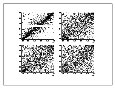
In figure 17, we have plotted the contours of the empirical copula for the assets AL and CU. We compare them with these computed with the gaussian distribution, i.e a gaussian copula with gaussian margins, and a gaussian copula (without assumptions on margins20_{). We remark that the gaussian copula fits better}

the empirical copula than the gaussian distribution!

Empirical copulas could be used to estimate dependence measures. For example, an estimation of the Spearman’s̺is

ˆ

̺= 12

T2₋₁

T

X

t1=1

T

X

t2=1

µ ˆ C µ_t 1 T, t2 T ¶

−t_T1t22

¶

(59)

18_{We have also}

C_(u

1,...,un−1) (un) =

ϕ_(n−1)(ϕ(u1) +. . .+ϕ(un))

ϕ(n−1)(ϕ(u1) +. . .+ϕ(un−1))

(54)

with

ϕ₍n)=

∂n ∂ unϕ

−1 ₍₅₅₎

19_{Definition (1) of the copula requires thatCis aN-increasing function (see footnote 3 page 4). This property means that there}

is a density associated toC.

Figure 17: Comparison of empirical copula, Gaussian distribution and Gaussian copula

Using the relationshipρ= 2 sin¡π

6̺

¢

between the parameter of gaussian copula and Spearman’s correlation, we deduce an estimate of the correlation matrix of the assets for the gaussian copula (Table 2). If we compare it with the correlation given in table 1 page 5, we show that they are close but different.

AL AL-15 CU NI PB

AL 1.00 0.87 0.52 0.41 0.36

AL-15 1.00 0.45 0.36 0.32

CU 1.00 0.43 0.39

NI 1.00 0.34

PB 1.00

Table 2: Correlation matrixρof the LME data

3.2.2 Identification of an Archimedean copula

Genest _and Rivest _{[1993] have developed an empirical method to identify the copula in the Archimedean} case. LetXbe a vector ofN random variables,Cthe associated copula with generator ϕand Kthe function defined by

K(u) = Pr{C(U1, . . . , UN)≤u} (60)

Barbe_,Genest_,Ghoudi _andR´emillard_{[1996] showed that}

K(u) =u+

N

X

n=1

(₋1)n ϕ

n_(u)

withκ_{n(u) =} ∂uκn−1(u)

∂uϕ(u) andκ0(u) =

1

∂uϕ(u). In the bivariate case, this formula simplifies to

K(u) =u−_ϕϕ_′(₍u_u)₎

A non parametric estimate ofKis given by

ˆ

K(u) = 1

T

T

X

t=1

1[ϑi≤u] (62)

with

ϑi=

1

T₋1

T

X

t=1

1_[xt

1<xi1,...,xtN<xiN] (63)

The idea is to fit ˆK by choosing a parametric copula in the family of Archimedean copulas (see Figure 18 for assetsALandCUpreviously defined).

Figure 18: QQ-plot of the functionK(u) (Gumbel copula)

3.3

Parametric estimation

In “Multivariate Models and Dependence Concepts”,Joe_{[1997] writes}

appropriate dependence structure, and otherwise be as simple as possible. The parameters of the model should be in a form most suitable for easy interpretation (e.g.,a parameter is interpreted as either a dependence parameter or a univariate parameter but not some mixture)...

In many applications, parametric models are useful in order to study the properties of the underlying statis-tical model. The idea to decompose the complex problems of multivariate modelling into two more simplified statistical problem is justified.

3.3.1 Maximum likelihood estimation

Let θ be the K×1 vector of parameters to be estimated and Θ the parameter space. The likelihood for observation t, that is the probability density of the observation t, considered as a function of θ, is denoted

Lt(θ). Let ℓt(θ) be the log-likelihood ofLt(θ). GivenT observations, we get

ℓ(θ) =

T

X

t=1

ℓt(θ) (64)

the log-likelihood function. ˆθML is the Maximum Likelihood estimator if

ℓ³θˆML

´

≥ℓ(θ) _∀θ_∈Θ (65)

We may show that ˆθMLhas the property of asymptotic normality (DavidsonandMacKinnon[1993]) and

we have _√

T³θˆML−θ0

´

−→ N¡

0,_J−1_(θ

0)¢ (66)

with_J(θ0) theinformation matrix of Fisher21.

Applied to distribution (3), the expression of the log-likelihood becomes

ℓ(θ) =

T

X

t=1

lnc¡

F1¡xt1

¢

, . . . ,Fn¡xtn

¢

, . . . ,FN¡xtN

¢¢ + T X t=1 N X n=1

lnfn¡xtn

¢

(70)

If we assume uniform margins, we have

ℓ(θ) =

T

X

t=1

lnc¡

ut1, . . . , utn, . . . , utN

¢

(71)

In the case of gaussian copula, we have

ℓ(θ) =₋T

2 ln|ρ| − 1 2

T

X

t=1

ςt⊤

¡

ρ−1₋I¢

ςt (72)

21_LetJ ˆ

θMLbe theT×KJacobian matrix ofℓt(θ) andHθˆMLtheK×KHessian matrix of the likelihood function. The covariance

matrix of ˆθMLin finite sample can be estimated by the inverse of the negative Hessian

varθˆML

=−HθˆML

−1

(67)

or by the inverse of the OPG estimator

varθˆML

=J_ˆ⊤ θMLJθˆML

−1

(68)

Another estimator called the White (or “sandwich”) estimator is defined by

varθˆML

=−HθˆML

−1

J⊤_ˆ θMLJθˆML

−HθˆML

−1

(69)

withςt=¡Φ−1(ut1), . . . ,Φ−1(utn), . . . ,Φ−1(utN)

¢

and the ML estimate ofρis also (Magnus_andNeudecker [1988])

ˆ

ρML=

1

T

T

X

t=1

ςt⊤ςt (73)

Unlike for gaussian copula, the estimation of the parameters for other copulas may require numerical optimisa-tion of the log-likelihood funcoptimisa-tion. This is the case of Student’s copula

ℓ(θ)_{∝ −}T

2 ln|ρ| −

µ_ν+N

2 ¶ T X t=1 ln µ

1 + 1

νς

⊤

t ρ−1ςt

¶ +

µ_{ν+ 1}

2 ¶ T X t=1 N X n=1 ln µ

1 + ς

2

n

ν ¶

(74)

The previous method, which we call the exact maximum likelihood method orEML, could be computational intensive in the case of high dimensional distribution, because it requires to jointly estimate the parameters of the margins and the parameters of the dependence structure. However, the copula representation splits the parameters intospecificparameters for marginal distributions andcommon parameters for the dependence structure (or the parameters of the copula). The log-likelihood (70) could then be written as

ℓ(θ) =

T

X

t=1

lnc¡

F1¡xt1;θ1¢, . . . ,Fn¡xtn;θn¢, . . . ,FN¡xNt ;θN¢;α¢+ T X t=1 N X n=1

lnfn¡xtn;θn¢ (75)

with θ = (θ1, . . . , θN, α). We could also perform the estimation of the univariate marginal distributions in a

first step

ˆ

θn = arg max T

X

t=1

lnfn¡xtn;θn¢ (76)

and then estimateαgiven the previous estimates

ˆ

α= arg max

T

X

t=1

lnc³F1

³ xt

1; ˆθ1

´

, . . . ,Fn

³ xt

n; ˆθn

´

, . . . ,FN

³ xt

N; ˆθN

´

;α´ (77)

This two-step method is called the method of inference functions for margins orIFM method. In general, we have

ˆ

θFML6= ˆθIFM (78)

In an unpublished thesis, Xu suggests “that the IFM method is highly efficient compared with ML method” (Joe_{[1997]). Using a close idea of theIFMmethod, we remark that the parameter vectorαof the copula could} be estimated without specifying the marginals. The method consists in transforming the data (xt

1, . . . , xtN) into

uniform variates (ˆut

1, . . . ,uˆtN), and in estimating the parameters in the following way:

ˆ

α= arg max

T

X

t=1

lnc¡ ˆ

ut1, . . . ,uˆtn, . . . ,uˆtN;α

¢

(79)

In this case, ˆαcould be viewed as the ML estimator given the observed margins (without assumptions on the parametric form of the marginal distributions). Because it is based on the empirical distributions, we call it thecanonical maximum likelihood method orCML.

Example 13 Let us consider two random variables X1 andX2 generated by a bivariate gaussian copula with

exponential and standard gamma distributions. We have

c(x1, x2) =p 1

1₋ρ2exp

µ

−1₂

µ

ς12+ 2ς1ς2+ς22

1−ρ2

¶ +1

2 ¡

ς12+ς22

¢ ¶

with

ς1 = Φ−1(1−exp (−λx1))

ς2 = Φ−1

µZ x2

0

xγ−1_e−x

Γ (γ) dx ¶

(81)

The vector of the parameters is also

θ= 

 λ γ ρ



 (82)

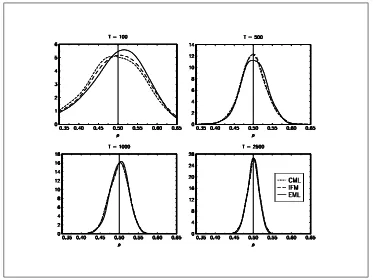
We perform a Monte Carlo study22 _{to investigate the properties of the three methods. In figure 19, we have}

reported the distributions of the estimators ρˆEML,ρˆIFM andρˆFML for different sample sizesT = 100,T = 500,

T = 1000andT = 2500. We remark that the densities of the three estimators are very close.

Figure 19: Density of the estimators

Remark 14 To estimate the parameterρof the gaussian copula with theCMLmethod23_{, we proceed as follows:}

1. Transform the original data into gaussian data:

(a) Estimate the empirical distribution functions (uniform transformation) using order statistics;

22_{The number of replications is set to 1000. The value of the parameters areλ= 2,γ= 1.5 andρ= 0.5.}

23_{Note that this isasymptoticallyequivalent to compute Spearman’s correlation and to deduce the correlation parameter using}

the relationship:

ρ= 2 sinπ 6̺

Figure 20: Empirical uniforms (or empirical distribution functions)

(b) Then generate gaussian values by applying the inverse of the normal distribution to the empirical distribution functions.

2. Compute the correlation of the transformed data.

Let us now use the LME example again. The correlation matrix estimated with theCMLmethod is given by table (3).

AL AL-15 CU NI PB

AL 1.00 0.85 0.49 0.39 0.35

AL-15 1.00 0.43 0.35 0.32

CU 1.00 0.41 0.36

NI 1.00 0.33

PB 1.00

Table 3: Correlation matrixρˆCMLof the gaussian copula for the LME data

3.3.2 Method of moments

We consider that the empirical momentsht,i(θ) depend on theK×1 vectorθof parameters. T is the number

of observations andm is the number of conditions or moments. Considerht(θ) the row vector of the elements

ht,1(θ), . . . , ht,m(θ) andH(θ) theT×mmatrix with elementsht,i(θ). Let g(θ) be am×1 vector given by

gi(θ) =

1

T

T

X

t=1

The GMM24criterion function Q(θ) is defined by:

Q(θ) =g(θ)⊤W−1g(θ) (85)

withW a symmetric positive definitem×mmatrix. The GMM estimator ˆθGMM corresponds to

ˆ

θGMM= arg min

θ∈ΘQ(θ) (86)

Like the ML estimators, we may show that ˆθGMMhas the property of asymptotic normalityand we have

√

T³θˆGMM−θ0

´

−→ N(0,Σ) (87)

In the case of optimal weights (W is the covariance matrix Φ ofH(θ) – Hansen_{[1982]), we have}

var³θˆGMM

´ = 1

T h

D⊤Φˆ−1Di−1 (88)

withD them_×K Jacobian matrix ofg(θ) computed for the estimate ˆθGMM.

“The ML estimator can be treated as a GMM estimator in which empirical moments are the components of the score vector” (Davidson _and MacKinnon_{[1993]). ML method is also a special case of GMM with} g(θ) =∂θℓ(θ) andW =IK. That is why var

³ ˆ

θGMM

´

is interpreted as an OPG estimator.

We may estimate the parameters of copulas with the method of moments. However, it requires in general to compute the moments. That could be done thanks to a symbolic software likeMathematicaorMaple. When there does not exist analytical formulas, we could use numerical integration or simulation methods. Like the maximum likelihood method, we could use the method of moments in different ways in order to simplify the computational complexity of estimation.

4

Financial Applications

4.1

Credit scoring

Main idea

We use the theoretical background on scoring functions developed by Gouri´eroux [1992]. We give a copula interpretation. Moreover, we discuss the dependence between scoring functions and show how to exploit it.

4.1.1 Theoretical background on scoring functions: a copula interpretation

4.1.2 Statistical methods with copulas

4.2

Asset returns modelling

Main idea

We consider some portfolio optimisation problems. In a first time, we fix the margins and analyze the impact of the copula. In a second time, we work with a given copula. Finally, we present some illustrations with different risk measures.

We then analyze the serial dependence with discrete stationary Markov chains constructed from a copula function (Fang, Hu and Joe [1994] and Joe [1996,1997]).

The third paragraph concerns continuous stochastic processes and their links with copulas (Dar-sow, Nguyen and Olsen [1992]).

4.2.1 Portfolio aggregation

4.2.2 Time series modelling

4.2.3 Markov processes

This paragraph is based on the seminal work of Darsow_,Nguyen_andOlsen_{[1992]. These authors define a} product of copulas, which is noted the_∗operation. They remark that “the _∗operation on copulas corresponds in a natural way to the operation on transition probabilities contained in the Chapman-Kolmogorov equations”.

4.2.3.1 The _∗ product and Markov processes

LetC1andC2be two copulas of dimension 2. Darsow,NguyenandOlsen[1992] define the product of

C1 andC2by the following function

C1∗C2 : I2 −→ I

(u1, u2) 7−→ (C1∗C2) (u1, u2) =

Z 1

0

∂2C1(u1, u)∂1C2(u, u2) du

(89)

where ∂1C and∂2C represent the first-order partial derivatives with respect to the first and second variable.

This product has many properties (Darsow_, Nguyen _and Olsen _[1992], Olsen_, Darsow _and Nguyen [1996]):

1. C1∗C2 is inC (C1∗C2 is a copula);

2. the∗ product is right and left distributive over convex combinations;

3. the_∗ product is continuous in each place;

4. the_∗ product is associative;

5. C⊥ _{is the null element}

C⊥_∗C=C_∗C⊥=C⊥ (90)

6. C+ _{is the identity}

C+_∗C=C_∗C+=C (91)

7. the∗ product is not commutative.

Using the fact that conditional probabilities of joint random variables (X1, X2) correspond to partial

derivatives of the underlying copula C(X1,X2), Darsow, Nguyen and Olsen [1992] investigate the

inter-pretation of the _∗ product in the context of Markov processes. Karatzas _and Shreve _{[1991] remind that} X =_{Xt,Ft;t≥0}is said to be a Markov process with initial distributionµif

(i) _∀A aσ-field of Borel sets inR

Pr_{X0∈ A}=µ(A) (92)

(ii) and fort_≥s

Pr_{Xt∈ A | Fs}= Pr{Xt∈ A |Xs} (93)

Darsow_,Nguyen_andOlsen_{[1992] prove also the following theorem:}

Theorem 15 Let X = {Xt,Ft;t≥0} be a stochastic process and let Cs,t denote the copula of the random

(i) The transition probabilitiesPs,t(x,A) = Pr{Xt∈ A |Xs=x}satisfy the Chapman-Kolmogorov equations

Ps,t(x,A) =

Z ∞

−∞

Ps,θ(x,dy)Pθ,t(y,A) (94)

for all s < θ < tand almost allx∈R_.

(ii) For all s < θ < t,

Cs,t=Cs,θ∗Cθ,t (95)

As Darsow_, Nguyen _and Olsen _{[1992] remark, this theorem is a new approach to consider Markov} processes:

In the conventional approach, one specifies a Markov process by giving the initial distribution µ

and a family of transition probabilities Ps,t(x,A)satisfying the Chapman-Kolmogorov equations.

In our approach, one specifies a Markov process by giving all of the marginal distributions and a family of 2-copulas satisfying (95). Ours is accordingly an alternative approach to the study of Markov processes which is different in principle from the conventional one. Holding the transition probabilities of a Markov process fixed and varying the initial distribution necessarily varies all of the marginal distributions, but holding the copulas of the process fixed and varying the initial distribution does not affect any other marginal distribution.

Darsow_,Nguyen_andOlsen_{[1992] recall thatsatisfaction of the Chapman-Kolmogorov equations}

is a necessary but not sufficient condition for a Markov process. They consider then the generalization of the_∗product, which is denotedC1⋆C2

IN1+N2−1 _{−→ I}

(u1, . . . , uN1+N2−1) 7−→ (C1⋆C2) (u) =

Z uN1

0

∂N1C1(u1, . . . , uN1−1, u)∂1C2(u, uN1+1, . . . , uN1+N2−1) du

(96) withC1 andC2two copulas of dimensionN1 andN2. They also prove this second theorem:

Theorem 16 LetX ={Xt,Ft;t≥0} be a stochastic process. LetCs,t andCt1,...,tN denote the copulas of the

random variables(Xs, Xt)and(Xt1, . . . , XtN). X is a Markov process if and only if for all positive integersN

and for all(t1, . . . , tN)satisfying tn< tn+1

Ct1,...,tN =Ct1,t2⋆· · ·⋆Ctn,tn+1⋆· · ·⋆CtN−1,tN (97)

4.2.3.2 An investigation of the Brownian copula

Revuz _andYor_{[1999] define the brownian motion as follows:}

Definition 17 There exists an almost-surely continuous processW with independent increments such that for eacht, the random variableW(t)is centered, Gaussian and has variancet. Such a process is called a standard linear Brownian motion.

It comes from this definition that

Ps,t(x,(−∞, y]) = Φ

µ y−x

√

t−s ¶

(98)

Moreover, we have by definition of the conditional distribution

withFtthe distribution ofW(t), i.e. Ft(y) = Φ¡y/√t¢. We have also

Cs,t(Fs(x),Ft(y)) =

Z x

−∞

Φ µ

y−z

√

t₋s ¶

dFs(z) (100)

With the change of variablesu1=Fs(x),u2=Ft(y) andu=Fs(z), we obtain

Cs,t(u1, u2) =

Z u1

0

Φ

µ√_tΦ−1_(u

2)−√sΦ−1(u)

√

t₋s

¶

du (101)

This copula has been first found byDarsow_,Nguyen_andOlsen_{[1992], but nobody has studied it. However,} Brownian motion plays an important role in diffusion process. That is why we try to understand the implied dependence structure in this paragraph.

We call the copula defined by (101) the Brownian copula. We have the following properties:

1. The conditional distribution Pr_{U2≤u2|U1=u1} is given by

∂1Cs,t(u1, u2) = Φ

µ√_tΦ−1_(u

2)−√sΦ−1(u1)

√

t₋s

¶

(102)

In the figure 22, we have reported the conditional probabilities for different sandt.

2. The conditional distribution Pr_{U1≤u1|U2=u2} is given by

∂2Cs,t(u1, u2) =

r t t₋s

1

φ(Φ−1_(u 2))

Z u1

0

φ

µ√_tΦ−1_(u

2)−√sΦ−1(u)

√

t₋s

¶

du (103)

3. The density of theBrownian copula is

cs,t(u1, u2) =

r t t₋sφ

µ√_tΦ−1_(u

2)−√sΦ−1(u)

√

t₋s

¶ ₁

φ(Φ−1_(u 2))

(104)

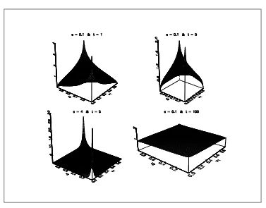
In the figure 23, we have represented the density for differentsand t.

4. TheBrownian copula is symmetric.

5. We have C0,t=C⊥,Cs,∞=C⊥ and limt→sCs,t=C+.

6. TheBrownian copula is not invariant by time translation

Cs,t6=Cs+δ,t+δ (105)

7. Let U1 and U2 be two independent uniform variables. Then, the copula of the random variables

³ U1,Φ

³√

t−1_sΦ−1_(U 1) +

p

t−1_(t−s)Φ−1_(U 2)

´´

is theBrownian copula Cs,t.

Let us now consider the relation between the marginal distributions in the context of stochastic processes. We have

Ft(Xt) = Φ

³√

t−1_sΦ−1_(F

s(Xs)) +

p

t−1_(t−s)ǫ

t

´

(106)

withǫta white noise process. It comes that

Xt=Ft−1

³

Φ³√t−1_sΦ−1_(F

s(Xs)) +

p

t−1_(t−s)ǫ

t

´´

Figure 21: Probability density function of the Brownian copula

In the case of the brownian motion, we retrieve the classical relation

Xt =

√

tΦ−1 µ

Φ µ√

t−1_sΦ−1

µ Φ

µ_X

s

√_s

¶¶

+pt−1_(t−s)ǫ

t

¶¶

= Xs+√t−sǫt (108)

Let us now consider the following marginal distributionsFt(y) =tν

³

y/q_vvt₋₂´with ν >2. By construction, we have this definition:

Definition 18 There exists an almost-surely continuous process Wν _{with independent increments with the}

same temporal dependence structure as the Brownian motionsuch that for eacht, the random variable

Wν_{(t)is centered, Student with variancet. Such a process is called a Student Brownian motion. W}ν_{(t)is then}

characterized by the marginals³tν

³

Wν_/q vt v−2

´´

t≥0and the copula

µZ u1

0

Φ

µ√_tΦ−1_(u

2)−√sΦ−1(u)

√

t₋s

¶ du

¶

t>s≥0

.

Figure 23 presents some simulations of these process. We remark of course that when ν tends to infinity, Wν

tends to the Gaussian brownian motion. We now consider now a very simple illustration. LetX(t) be defined by the following SDE:

½

dX(t) = µX(t) dt+µX(t) dW(t)

X(t0) = x0 (109)

The solution is the Geometric Brownian motion and the diffusion process representation is

X(t) =x0exp

µµ

µ−1₂σ2 ¶

(t−t0) +σ(W(t)−W(t0))

¶

(110)

We consider now a new stochastic processY (t) defined by

Y(t) =x0exp

µµ µ₋1

2σ

2

¶

(t₋t0) +σ(Wν(t)−Wν(t0))

¶

(111)

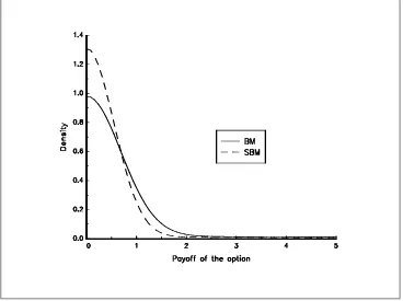
What is the impact of introducing these fat tailed distributions in the payoff of aKOCoption ? The answer is not obvious, because there are two phenomenons:

1. First, we may suppose that the probability to be out of the barriers Land H is greater for the Student brownian motion than for the brownian motion

Pr_{Y (t)_∈[L, H]_{} ≤}Pr_{X(t)_∈[L, H]_} (112)

2. But we have certainly an opposite influence on the terminal payoff (K is the strike)

Prn(Y (T)₋K)+_≥go_≥Prn(X(T)₋K)+_≥go (113)

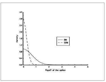
In figure 24, we have reported the probability density function of theKOCoption with the following parameter values : x0= 100,µ= 0,σ= 0.20,L= 80,H= 120 andK= 100. The maturity of the option is one year. For

the student parameter, we useν= 10. In figure 25, we useν= 4.

4.2.3.3 Understanding the temporal dependence structure of diffusion processes

The Darsow-Nguyen-Olsen approach is very interesting to understand the temporal dependence structure of diffusion processes. In this paragraph, we review different diffusion processes and compare their copulas.

Figure 23: Simulations of a Brownian motion (BM) and of a Student Brownian motion (SBM

Figure 25: Density of the payoff of theKOCoption (ν = 4)

Proof. We have

Ps,t(x,(0, y]) = Φ

Ã

lny₋lnx₋¡ µ₋1

2σ 2¢

(t₋s)

σ√t₋s

!

(114)

Then, it comes that

Cs,t(Fs(x),Ft(y)) =

Z x

0

Φ Ã

lny₋lnz₋¡ µ₋1

2σ 2¢

(t₋s)

σ√t−s

!

dFs(z)

withFt(y) = Φ

µ

lny−lnx0−(µ−12σ 2_)t

σ√t

¶

. With the change of variablesu1=Fs(x),u2 =Ft(y) andu=Fs(z),

we have

lnz₋lnx0−

µ µ₋1

2σ

2

¶

s = σ√sΦ−1_(u)

lny₋lnx0−

µ µ₋1

2σ

2¶_{t = σ}√_tΦ−1_(u 2)

lny₋lnz₋ µ

µ₋1

2σ

2¶_(t

−s) = σh√tΦ−1(u2)−√sΦ−1(u)

i

(115)

The corresponding copula is then

Cs,t(u1, u2) =

Z u1

0

Φ µ√

tΦ−1_(u

2)−√sΦ−1(u)

√

t₋s

¶

Note that we could prove the previous theorem in another way. LetCs,tbe the copula of the random variables

W(s) andW(t). Let us consider two functions α(x) andβ(x) defined as follows:

α(x) = x0exp

µµ µ₋1

2σ

2¶_(s

−t0) +σx

¶

β(x) = x0exp

µµ

µ−1₂σ2 ¶

(t−t0) +σx

¶

(117)

Because these two functions are strictly increasing, the copula of the random variablesα(W(s)) andβ(W(t)) is the same as the copula of the random variablesW(s) andW(t).

Definition 20 An Ornstein-Uhlenbeck process corresponds to the following SDE representation

½

dX(t) = a(b₋X(t)) dt+σdW(t)

X(t0) = x0 (118)

Using Ito calculus, we could show that the diffusion process representation is

X(t) =x0e−a(t−t0)+b

³

1₋e−a(t−t0)´_+σ

Z t

t0

ea(θ−t)dW(θ) (119)

By definition of the stochastic integral, it comes that the distribution Ft(x)is

Φ Ã

x−x0e−a(t−t0)+b¡1−e−a(t−t0)¢

σ

√

2a

√

1₋e−2a(t−t0)

!

(120)

Theorem 21 The Ornstein-Uhlenbeck copula is

Cs,t(u1, u2) =

Z u1

0

Φ µ_~(t

0, s, t) Φ−1(u2)−~(t0, s, s) Φ−1(u)

~_{(s, s, t)}

¶

du (121)

with

~_{(t0, s, t) =}p_e2a(t−s)_−e−2a(s−t0) (122) Proof. We have

Ps,t(x,(−∞, y]) = Φ

Ã

y₋xe−a(t−s)_+b¡

1₋e−a(t−s)¢

σ

√

2a

√

1−e−2a(t−s)

!

(123)

Then, it comes that

Cs,t(Fs(x),Ft(y)) =

Z x

−∞

Φ Ã

y−ze−a(t−s)_+b¡

1−e−a(t−s)¢

σ

√

2a

√

1₋e−2a(t−s)

!

dFs(z) (124)

Using the change of variablesu1=Fs(x),u2=Ft(y) andu=Fs(z), it comes that

y−ze−a(t−s) = x0e−a(t−t0)−b

³

1−e−a(t−t0)´_+√σ

2a p

1−e−2a(t−t0)Φ−1(u₂)−

e−a(t−s)

·

x0e−a(s−t0)−b

³

1₋e−a(s−t0)´₊ σ

√

2a p

1₋e−2a(s−t0)Φ−1(u)

¸

= −b³1−e−a(t−s)´+

σ

√

2a hp

1−e−2a(t−t0)_Φ−1_(u

2)−e−a(t−s)

p

1−e−2a(s−t0)_Φ−1_(u)

i

Then, we obtain a new expression of the copula

Cs,t(u1, u2) =

Z u1

0

Φ Ã√

1−e−2a(t−t0)_Φ−1_(u

2)−e−a(t−s)

√

1−e−2a(s−t0)_Φ−1_(u)

√

1₋e−2a(t−s)

!

du (126)

The Ornstein-Uhlenbeck copula presents the following properties:

1. The Brownian copula is a special case of the Ornstein-Uhlenbeck copula with the limit function

lim

a−→0

~_{(t0, s, t) =}√_{t−t0 (127)}

2. The conditional distribution Pr{U2≤u2|U1=u1} is given by

∂1Cs,t(u1, u2) = Φ

µ_~

(t0, s, t) Φ−1(u2)−~(t0, s, s) Φ−1(u1)

~_{(s, s, t)}

¶

(128)

3. The conditional distribution Pr{U1≤u1|U2=u2} is given by

∂2Cs,t(u1, u2) =

~_{(t0, s, t)} ~_{(s, s, t)}

1

φ(Φ−1_(u 2))

Z u1

0

φ µ_~

(t0, s, t) Φ−1(u2)−~(t0, s, s) Φ−1(u)

~_{(s, s, t)}

¶

du (129)

4. The density of the Ornstein-Uhlenbeck copula is

cs,t(u1, u2) =

~_{(t0, s, t)} ~_{(s, s, t)}φ

µ_~(t

0, s, t) Φ−1(u2)−~(t0, s, s) Φ−1(u1)

~_{(s, s, t)}

¶ ₁

φ(Φ−1_(u 2))

(130)

We have represented the density of the Ornstein-Uhlenbeck copula for different values ofsandt(t0is equal

to 0). We could compare them with the previous ones obtained for the Brownian copula. We verify that

lim

a−→∞Cs,t(u1, u2) =C

⊥ ₍₁₃₁₎

but we have

lim

a−→−∞Cs,t(u1, u2) =C

+ ₍₁₃₂₎

In order to understand the temporal dependence of diffusion processes, we could investigate the properties of the associated copula in a deeper way. We have reported in figures 28 and 29 Spearman’s rhos for Brownian and Ornstein-Uhlenbeck copulas.

Remark 22 A new interpretation of the parameterafollows. For physicists,ais the mean-reverting coefficient. From a copula point of view, this parameter measures the dependence between the random variables of the diffusion process. The bigger this parameter, the less dependent the random variables.

4.3

Risk measurement

Main idea

Figure 26: Probability density function of the Ornstein-Uhlenbeck copula (a=1₄)

Figure 28: Spearman’s rho (s= 1)