Rule Extraction from Support Vector Machines: A Geometric Approach. Technical Report

City, University of London Institutional Repository

Citation: Renou, L. and d'Avila Garcez, A. S. (2008). Rule Extraction from Support Vector

Machines: A Geometric Approach. Technical Report (TR/2008/DOC/01). Department of

Computing, City University London: .

This is the published version of the paper.

This version of the publication may differ from the final published

version.

Permanent repository link: http://openaccess.city.ac.uk/4111/

Link to published version: TR/2008/DOC/01

Copyright and reuse: City Research Online aims to make research

outputs of City, University of London available to a wider audience.

Copyright and Moral Rights remain with the author(s) and/or copyright

holders. URLs from City Research Online may be freely distributed and

linked to.

Rule Extraction from Support Vector Machines: A Geometric

Approach

Lu Ren and Artur Garcez

Department of Computing, City University London

cf529@soi.city.ac.uk

,

aag@soi.city.ac.uk

Abstract— This paper presents a new approach to rule

extraction from Support Vector Machines. SVMs have been

applied successfully in many areas with excellent generalization results; rule extraction can offer explanation capability to SVMs. We propose to approximate the SVM classification boundary through querying followed by clustering, searching and then to extract rules by solving an optimization problem. Theoretical proof and experimental results then indicate that the rules can be used to validate the SVM results, since maximum fidelity with high accuracy can be achieved.

I. INTRODUCTION

In recent years, Support Vector Machines (SVMs) have been utilised in many applications offering excellent gener-alization results. In many cases, however, developers prefer not to use SVMs because of their inability to explain how the results have been obtained. For example, if used for stock predictions, an SVM can provide users with a mechanism for forecasting, but the knowledge associated with the pre-dictions may be incomprehensible; users may have to trust the prediction results while unable to validate the rules of the data.

The area of rule extraction addresses the above problem. By extracting rules from SVMs, we can explain the reasoning process and validate the learning system. Rule extraction helps, therefore, to integrate the symbolic and connectionist approaches to AI, offering ways of combining the statistical nature of learning with the logical nature of reasoning.

Since the early 1990s, various algorithms to extract rules from trained neural networks have been proposed, notably [4], [2], [17], [11], [14], [12], [5]. Some of these search for rules by decomposing the networks and extracting rules for each unit, and some extract rules directly from the input-output values of the networks, thus treating them as black-boxes. Recently, SVMs started to be considered for rule extraction because of their excellent generalization capability. Angulo et al [19] used support vectors and prototypes to draw regions indicating an equation rule or interval rule. Barakat and Diererich [15] used support vectors to construct synthetic data, feed the data into a decision tree learner, and extract rules. Fung et al [6] proposed an algorithm that approximates linear SVM hyperplanes by a set of rules.

In our opinion, a satisfactory extraction method, striking a balance between the need for correctness and efficiency, is still lacking. Most of the extraction methods are designed for specific architectures and training sets, or are affected by the tradeoff between efficiency and rule accuracy. In this

paper, we tackle both of these issues by proposing a new any-time rule extraction algorithm, which uses the SVM as an oracle (black-box) and synthetic data for querying and rule extraction, thus making fewer assumptions about the training process and the SVM training data. The algorithm is not restricted to a specific SVM classifier such as the linear classifier considered in [6], neither does it depend on the availability of specific training sets for rule extraction. Instead, it seeks to capture the information encoded in the geometry of the SVM by approximating the region separated by the SVM classification boundary through querying [12] and searching, and then extracting rules by solving an optimization problem, which we describe in detail in the sequel. We also prove the soundness and completeness of our approach, and run experiments and compare our approach with other extraction methods. We examined rule accuracy, fidelity and comprehensibility in two applications: the iris flower dataset and the breast cancer-wisconsin dataset. The results indicate the correctness of our approach through maximum fidelity.

The paper is organised as follows: Section 2 gives a brief introduction to SVMs. Section 3 describes our new extraction algorithm. Section 4 presents the proofs. Section 5 contains the experimental results, and Section 6 concludes and discusses directions for future work.

II. SUPPORTVECTORMACHINES

We consider the problem of classifying n points in the

m-dimensional input space Rm_{. Consider the training data}

set {(xi, yi)}, i = 1, ..., n,yi ∈ {1,−1} and xi ∈ Rm. In

the case of linear SVMs the decision function is a separating hyperplanef(x) =sign(w·x+b). The optimal classification hyperplane that maximizes the distance between classA+=

1 and A− = −1 can be found by minimizing 1/2kwk2

subject to yi(w·xi+b)≥1.

The LagrangianJ below has been introduced to solve this problem:J =1₂wTw−Σn_i=1αi(yi(w·xi+b)−1), whereαi≥ 0is known as the lagrange multiplier. With respect towand b, minimizingJ leads tow= Σsv_i=1αiyixiandΣni=1αiyi= 0

wheresv is the number of support vectors [21]. By making some substitutions, we arrive at the hyperplane decision function f(x) =sign(Σsv_i=1αiyihxi·xji+b),j = 1, ..., n,

wherehidenotes inner product.

kernel functionsK(x, x0_{) =hΦ(x)·Φ(x}0_{)i, all the necessary}

operations in the input space may be carried through, and the decision function can bef(x) =sign(Σsv

i=1αiyiK(xi,xj) + b). For more details on SVMs, see [21].

III. GEOMETRICSVM RULEEXTRACTION

Most rule extraction algorithms suffer from a lack of generality, a balance between correctness and fidelity, or both. In this section, we present a novel rule extraction al-gorithm called Geometric and Oracle-Based Support Vector

Machines Rule Extraction (GSVMORC), which is designed

to alleviate these limitations. GSVMORC utilizes the points on the SVM classification boundary and synthetic training instances to construct a set of optimized hypercube rules. The area covered by those rules is maximized and approximates the area of interest. The definitions of the hypercube rule and the area of interest are given as follows.

Definition 3.1: Hypercube Rule: It is said that an

m-dimensional hypercubeH characterizes a rule if every point in the scope ofH falls into the same class classified by the SVM network. More precisely:

H =

n

xi

¯

¯^_{lj ≤xij ≤uj →Ak,1≤j ≤m}o

wherexi= [xi1, ..., xim],lj anduj are the upper and lower

bounds on H. Ak indicates a class label, and m is the

dimension of the input space.

Definition 3.2: Area of Interest. This is the whole region

covered by a class Ak in the input space.

I(Ak) =©xi

¯

¯ _{the class of xi =Ak, lj≤xij≤uj,}ª_,

where 1 ≤ j ≤ m, i ≥ 1, xi is an m-dimensional input

vector. uj and lj are the upper and lower bounds of xij. xij refers to the jth dimension of xi. There is no vector

xi∈I(Ak)such that the classification ofxiequals the other

class rather than Ak.

The aim of GSVMORC is to use the classification boundary and synthetic training instances to extract the hypercube rules without considering the inner structure and the support vectors of the SVM network. It treats the SVMs as oracles, and makes fewer assumptions about the architecture and training process, hopefully being applicable to other non-symbolic learning methods. All we assume is that an SVM is given which we can query and find the classification it gives for input vectors xi. After querying, a clustering

process is imposed on those inputs xi with the same yi,

in order to group them into a set of clusters. Then, by means of a binary search algorithm, we look for the pointsP

that lie on the SVM classification boundaries. Subsequently, an initial optimal rule set can be extracted for the points in P and synthetic training instance set by solving an optimization problem whereby we attempt to find the largest consistent hypercubes in the input space. Finally, several post-processing measures are applied to this initial rule set in order to derive (a relatively small number of) generalized rules from. In what follows, we explain each of the above steps of our extraction algorithm.

Querying. The generality of GSVMORC is because it

generates a subset of synthetic training inputs to query the SVMs, which then returns back the class labels of the inputs. We use a random data generator to produce a large amount of inputs. Only those inputs locate in the range of the input space, and their values of a density estimator M(x) are larger than a user-defined constraint c1 are retained. Unlike TREPEN [13] which uses the kernel density estimates

of individual features, GSVMORC uses multivariate kernel density estimates which takes into account the relations

within features. M(x) used by GSVMORC models the

probability density function for inputs xas:

M(x) = 1 N

N

X

i=1

1

Qm j=1hj

[ 1

(√2π)me

−1

2(k

x−Xi h k)]

where Xi are the given training samples, 1 ≤ i ≤ N. h= [h1, h2, ...hm] is a vector of bandwidth such thath=

[_(m+2)4 _N]m1+4σ_whereσ_{is standard deviation of the training}

samples. Figure 1 contains the input generation algorithm.

DRAWINPUTS

Input: a constraintc1, the lower and upper bounds of the input spaceLandU, a random data generatorg(x), a density estimator

M(x)and the number of iteration timesT

Output: the input setx={xi:i≥1} (1) Initialize the input setx

(2) GenerateT random data{xi: 1≤i≤T}based ong(x) (3) for each iterationi < T do

(4) IfL≤xi≤U then (5) CalculateM(xi) (6) ifM(xi)> c1then (7) x:=xSxi

Fig. 1. The DRAWINPUTS function: call a random data generatorg(x)to create uniformly distributed data; use a density estimatorM(x)to reserve those data whose probabilities are larger than an arbitrary number c1. Meanwhile, the outputs should lie between_. LandU

After obtaining those synthetic inputs{xi, i≥1}, we treat

them as the inputs of the SVMs; the SVMs are considered as oracles 1. Suppose we have an SVM computing function f(x). For each input xi, we feed xi into the SVM and

get the corresponding output yi = f(xi). The instances {(xi, yi), i≥1} are created. Note that the distanced from

xi to the separating hyperplane is also obtained when SVM

answer the queries from xi.

The last step in querying is called SELECTINSTANCE. GSVMORC defines a factornso that it is much more flexible in its ability to choose differing sizes of instances. In order to select the instances with much higherM(x), thosexi(i≥1)

1_{Notice that the SVM is considered as a black box. All we need to know}

are key input-output patterns, rather than the inner structure. This complies with Thrun’s desideratum for a general rule extraction method of no training

requirement[4]. The querying process makes our approach independent of

with the same class label are sorted first. Suppose that there are CN classes involved in the classification problem and that the number of xi for each class is n(G). In this case,

we choose the first n/CN instances, or the whole group of instances ifn(G)< n/CN, to build up the synthetic training instance setS.

One key issue in querying is how to know the classes which are needed to be classified in a general way. GSV-MORC still generates a large amount random data Z = {z1, ...,zh}2, which are uniformly distributed in the input

space. These data Z are then input into the SVM network to acquire class labels for them. For largeh, we believe that the data in Zare able to spread throughout the input space. Therefore, a set of classes (A={Ak|1≤k≤CN, CN is

the total number of classes }) can be obtained after filtering the duplicates.

Clustering. Since there must be a classification boundary

between different classes, we can find the points lying on the classification boundary between pairs of data for different classes. However, for a large number of training data, if we search each pair of data for different classes, this may lead to high complexity. Hence, we use clustering to create a balance between the complexity and prediction accuracy. A cluster Ccan be defined as a subset of training dataS={(xi, yi)},

with the same class yi.

We use hierarchical clustering on S. It starts by con-sidering each individual point as a cluster, and it merges the clusters by measuring the distance between two clusters of data which have the same class labels. Because the mergence of the clusters is relevant only to those training instances that have the equivalent class, just the inputs xi

are involved in the distance calculation. Our approach uses one of the following linkage functions: Single linkage, uses the smallest distance between data xr_i and xs_j in the two clusters r ands. If the size ofr and sare nr andns then d(r, s) =min(dist(xr

i,xsj)), i∈ (1, ..., nr), j ∈ (1, ..., ns);

Complete linkage, uses the largest distance between dataxr

i

and xs

j in the two clusters r and s such that d(r, s) = max(dist(xr

i,xsj)).

In order to reduce the randomness of the number of clusters, a stopping criterion is defined for the clustering process. Given q clusters {rh, h = 1,2, ..., q}, the classes

of the clusters are identical, and the number of data in each cluster rh is nrh. It is obvious that the mean and variance

of each cluster relate to the data xi,1≤i≤nrh inside this

cluster. Hence, the meanmrh _{of each clusterr}

h is:

mrh ₌ 1

nrh

nrh

X

i=1

xi

and the variancesrh _is

srh ₌ 1

nr nrh

X

i=1

(xi−mrh)2

2_{his an arbitrary large integer.}

Hence, the intra-cluster deviation is defined as follows:

sintra ₌

v u u tXq

h=1

(srh∗p(rh)) ₍₁₎

wherep(rh) =Pqnrh h=1nrh.

And the inter-cluster mean and deviation are specified in Equation 2.

minter= q

X

h=1

(mrh_{∗p(rh)) (2a)}

sinter =

v u u tXq

h=1

[(mrh−minter)2∗p(rh)] _(2b)

Definition 3.3: The stopping criterion D is the rate

be-tweensintra andsinter.

If s_sintrainter > ², then GSVMORC will stop merging the data

further. Note that ²is a user-defined parameter.

Searching.The searching step searches for and

lo-cates the points on the decision boundaries. Given clus-ters P1, P2, ...Pa which fall into class A+, and clusters N1, N2, ...Nb which fall into class A−, we use Zhang and

Liu’s measure [24] to automatically look for the points on an SVM’s decision boundary3_.

We consider all pairs (p, n) s.t. p∈ Pj(1 ≤j ≤a) and n ∈ Nk(1 ≤k ≤ b). For each p, we find a corresponding pointnwhose distance topis minimum. And for eachn, we find a corresponding pointpwhose distance tonis minimum. As described in querying section, the distance from any point to the SVM hyperplane is one of the outputs by querying the SVM network. Let d1 represent the distance from pto the hyperplane and d2 represent the same for n. In order to find the point lying on the hyperplane, a binary search procedure is performed on (p, n). In other words, if |d1− d2| > ε, the mid-point q between p and n is chosen. The SVM network classifiesqand computes the distance between qand the hyperplane. If the class ofqequals that ofp, thenp is replaced byq; otherwise,nis replaced byq. The process carries on until |d1−d2|< εis achieved, where εdenotes an arbitrary small number.

Extracting. The main idea of our rule extraction approach

is to find a set of optimal rules that 1) covers the maximum area of the area of interest and 2) covers the largest cardi-nality of synthetic instances at the same time.

Suppose that there are a set of pointsXlying on the SVM decision boundary, where X is the result of searching, a set of synthetic training instances S generated from querying for classes A={Ap,1≤p≤CN}, and the SVM function f(x).

To realize the first goal of the rule extraction algorithm, we try to solve the following optimization problem:

maximize

m

Y

i=1

(xi−x0i) (3a)

3_{Notice that for simplicity we have been consideringP= 2classes, but}

subject to l≤x≤u (3b)

Z u

l

(f(x)−Ap)dx= 0 (3c)

where x0i denotes the ith element of vector x0 ∈ X (x0

indicates a starting point),xiis theithelement of x,landu

are the m-dimensional vectors giving lower and upper bounds to this optimization problem.

The objective function (Equation 3a) aims to maximize the volume of the hypercube that a rule covers, and it has two constraints. One is a bound constraint to limit the optimalx∗ in a given area, while the other is a nonlinear constraint that is used to exclude the points that have different class labels. The values of l and u in Equation 3b can be calculated based on the lower and upper bounds of the input space. For example (see Figure 2(a)), suppose the scope of the input space is [L1, L2]≤x ≤[U1, U2], and x0 = [x01,x02] is a

point lying on the SVM boundary. Note that when we change 4x01onx01or−4x02onx02(4x01,4x02 ≥0) the SVM

classification on x0 is class Ap. Hence, it is reasonable to

assume that an optimal point can be found and that a rule for class Ap in a rectangle between points x0 and[U1, L2]can be constructed. Here, [U1, L2] is defined as an orientation forx0.landuare then narrowed down tol= [x01, L2]and

u= [U1,x02].

If more than one orientation is found for classAp, then the

principal orientations have to be selected. Let v = [v1, v2] stand for an orientation for x0. In the above example,v=

[U1, L2]. Selecting the orientations forx0 involves deciding how to compute the significance of each orientation. Equa-tion 4 shows condiEqua-tional probability estimaEqua-tion that GSV-MORC uses to determine the significance of each orientation. The estimation represents the probability distribution of x lying in the area betweenvandx0, given classAp. In

Equa-tion 4, P(min(v,x0) ≤ x ≤ max(v,x0)

T

class = Ap)

indicates the probability of x falling into the area between

v as well as belonging to classAp, andP(class = Ap)is

the possibility that the classification of x equalsAp. Assume

that the distribution of synthetic training examples is similar to that of the problem domain. Hence, the probabilities P(min(v,x0) ≤ x ≤ max(v,x0)

T

class = Ap) and P(class = Ap)could be worked out from the synthetic data set. The value ofP(min(v,x0)≤x≤max(v,x0)|class = Ap) is then calculated by dividing P(min(v,x0) ≤ x ≤

max(v,x0)

T

class = Ap) by P(class = Ap). The end result is that those orientations that have the maximum probabilities are selected as the principal orientations on x.

P(min(v,x0)≤x≤max(v,x0)|class=Ap)

= P(min(v,x0)≤x≤max(v,x0)

T

class=Ap) P(class = Ap) (4)

As presented in Equation 3c, the nonlinear constraint is a multi-dimension integral on a linear/nonlinear function. GSVMORC uses a quasi-Monte Carlo method [22] to ap-proximate the integration because it is a superior method

with many advantages such as improved convergence and more uniformity. Therefore, the hypercube H is considered to be composed of the points that are uniformly distributed as:

1 n

n

X

i=1

|f(ai)−Ap| ≈

Z _u

l

|f(x)−Ap|dx

whereaiis a low-discrepancy sequence inside the hypercube [l, u], where 1 ≤i ≤ n, and n here means the number of points selected for approximation in the H. The estimation error then becomes,

²=

¯ ¯ ¯ ¯ ¯

Z _u

l

|f(x)−Ap|dx−1 n

n

X

i=1

|f(ai)−Ap|

¯ ¯ ¯ ¯ ¯

From the above, it can be shown that the largern is, the closer the approximation approaches the integral. It is clear that the complexity increases with the rise ofn. Therefore, in order to strike a balance between error estimation, fidelity, accuracy prediction and complexity, a proper n has to be chosen. In the cross-validation experiments, we found n=

1000as a suitable number for our benchmark datasets. With this, the standard pattern search algorithm is applied to obtain a solutionx∗ _{to the optimization problem. Charles}

and Dennis analyze the generalization of the pattern search by evaluating the objective function [1]. After obtaining the optimal point x∗, together with the starting point x0, the antecedents of a rule can be constructed by picking the minimum and maximum values of x∗ and x0, as shown in Figure 3. Figure 2(a) gives an example of a hypercube rule with the starting point x0.

Finally, to find the set of rules covering all the synthetic training instances, Equation 3 is used again, and in it,x0 is replaced with s ∈ S (see Figure 2(b)). The process is the same, which ensures the extracted rules cover most of the synthetic training instances as well as the maximum area of the area of interest.

Figure 3 summaries the rule extraction algorithm and its associated rule generation algorithm, as discussed above.

The rule set obtained from extracting may contain over-lapping rules, for which a set of post-processing measures in the next section are employed to solve this problem.

s

x0’(x0’1, x0’2)

[x0’1, x2] < x < [x1, x0’2] Ap

x* (x1,x2)

X2

X1

(a)

[x1, l2] < x < [u1, x2] Ap

x* (x1, x2)

x’

s (u1, l2)

X2

X1

(b)

Fig. 2. left: extracting the rule from the starting point[x01,x02]which

Extracting

Input: A set of pointsX on the SVM boundary obtained from the searching step; a set of training dataS obtained from querying step and the class labelAp.

Output: A set of rulesR={r},

wherer=Vli≤xi≤ui→Ap,1≤i≤m (1) for eacht∈X

(2) Construct the lower and upper boundl andu by finding the orientations ofx

(3) Apply pattern search algorithm [1]withx0=tto obtainx∗

(4) Call rule generation algorithm with parametersx∗

andx0 to construct a ruler and makeR :=∪r (5) for eachs∈S and its correspondingt∈X

(6) Construct the lower and upper boundl andu

by finding the orientations ofs

(7) Apply pattern search algorithm [1] withx0=sto obtainx∗0

.

(8) Call rule generation algorithm with parametersx∗0 ands

to construct a ruler0

and makeR:=R∪r0

Rule Generation Algorithm Input: m-dimensional pointsx∗

andx0

Output: a ruler

(1) Let lower boundl= [min(x∗

1,x01), ..., min(x

∗

m,x0m)]

(2) Let upper boundu= [max(x∗

1,x01), ..., max(x

∗

m,x0m)]

(3) Generater=Vli≤xi≤ui→Ap,1≤i≤m

Fig. 3. Rule extraction algorithm

Post-Processing. The purposes of these post-processing

measures are to detect generalized rules, to prune rules with high error estimation and to construct non-overlapping rules with high coverage rate.

The notions of non-overlapping and coverage rate are defined as follows.

Definition 3.4: Non-overlapping Rule: Given two rules,

r1=

V

ai ≤xi≤bi→Apandr2=

V

ci≤xi≤di→Ap, r1 and r2 are said to be non-overlapping iff bi ≤ ci or ai≥di, for anyi,1≤i≤m.

Definition 3.5: Coverage rate is the rate between the

num-ber of testing data that are predicted correctly by a rule and the entire testing data.

1) Rule Extending: Given that the input space of a

prob-lem domain is from [L1, ..., Lm] to[U1, ..., Um] and that of a rule is r = [l1, ..., lm] ≤x ≤[u1, ...um]→Ap, the

rule-extending step attempts to extendrinto a larger scope. At the same time, the new ruler0_{still satisfies the constraint that the}

area covered byr0_{belongs to the same class. To exhaustively}

find all the potential rules in an extended scope, a topology is used to achieve this.

Let the original value of r be 0 and the new value of a rule be 1. For example, if the 1st dimension of r is extended to L, then r becomes l0 = [L1, l2, ..., lm] ≤ x≤ u0 _{= [u}

1, ..., um] →Ap. Hence, the new value [L1, u1] on dimension one is regarded as 1. The definition of topology is defined as follows.

Definition 3.6: Topology: An arrangement in which each

000

001 010

100

101 011

110

111

Fig. 4. Ordering on extending to the edge of the problem domain.

element means that the value of every dimension is mapped to0 or 1according to the above regulations.

Figure 4 shows an example of a topology where the dimension of the input space is 3.

We assume that the rule r initially constructs a rule set R. The function hasm−1 iterations, and for each iteration, rj inR is picked, and every dimension of rj is extended,

where 1 ≤ j ≤ n and n is the number of rules in R. At the first iteration, there is only one rule in Rthat isrj=r, j= 1. Subsequently, each dimensioniis extended toLi, and

the new value [Li, ui] is verified if it satisfies the constraint

1

n

Pn

i=1(|f(xi)−Ap|) = 0. Next, for the same dimension,r

is then extended toUi, and a similar verification is performed

on this new value. If there is any extension on the value of the ith _{dimension of r, the new rule r}0 _{is kept for the next}

iteration. After going through each dimension of rj, all the

new rules,r0, are put together for a new rule set R. Finally, if the value of theith_{dimension equals the scale of}

the input space, which is believed to be applicable throughout the total range of theith_{dimension, GSVMORC then filters}

this dimension from the antecedents of the rule.

The complexity becomes exponential if the algorithm goes through every element in the topology. It increases with the rise of the dimensionality of the input space and even grows to be intractable in the worst case. Hence, in practice, an optimizing measure known as the cracking of topology has been adopted.

Firstly, the definition of a clash of the topology is given. A

clash is an occurrence when the new region of a rule consists

of the points for another class. The rule can be represented as an element in the topology.

When a clash is identified on a certain element, the rule-extending process would not continue on with the remaining elements that have connections with the element that has the

clash. This is called cracking of topology.

Consider a three-dimensional problem. The antecedents of an initial rule are interpreted as 000. It is then easy to make a structure in the order of Figure 4. Given such an ordering, some conclusions can be drawn. If an element in Figure 4 deviates from _n1Pn_i=1|f(ai)−Ap| = 0, then

a clash would be detected, which indicates that no other element along the ordering of this element would satisfy

1

n

Pn

2) Rule Pruning: The rule pruning stage aims to prune

those rules that have a relatively large estimated error. GSVMORC uses a t-test to analyze the null hypothesis that the mean of the estimated value and the expected value of the integral of a rule r are equal, that is the mean of the estimated value equals 0.

As GSVMORC uses quasi-Monte Carlo method to ap-proximate the integration function in Equation 3c, there is a potential error between the approximation value and the integral. Most existing studies use the Koksma-Hlawka inequality [3] to state the limit of the integration error.

¯ ¯ ¯ ¯ ¯

1 n

n

X

i=1

|f(xi)−Ap| −

Z _U

L

|f(x)−Ap|

¯ ¯ ¯ ¯

¯≤V(f)D

∗

N

However, it is usually difficult to calculate the total vari-ation V(f), which makes it problematic to estimate error through Koksma-Hlawka inequality.

Morohosi and Fushimi [7] introduce a statistical method for quasi-Monte Carlo error estimation. The rule pruning of GSVMORC is based on their method. The general scheme of the method is as follows.

Suppose a rule r with an area ranging from l to u, M data sets {x(_ij)}n

i=1, where j = 1, ..., M, l ≤x (j)

i ≤uand {x(_ij)}n

i=1 is a set of pseudorandom data. For each data set, the value of Equation 5 is computed.

S(j)₌ 1 n

n

X

i=1

|f(xi)−AP|, j= 1, ..., M (5)

The estimate of the meanIˆis calculated by

ˆ I= 1

M M

X

j=1

S(j) ₍₆₎

so that the error of the integral is estimated using the variance of the evaluated values.

ˆ

σ2₌ 1 M(M −1)

M

X

j=1

(S(j)−Iˆ)2 (7)

Hence, the t-test turns out to be:

t= I_σˆˆ

√

M

(8)

GSVMORC sets a significance level to specify how close the approximation value is to the expected value 0. If t is larger than the standard value at the significance level, the rule is rejected. Otherwise it is accepted.

Those rules rejecting the null hypothesis are removed. Therefore, GSVMORC’s pruning is able to ensure that GSVMORC approximates the behavior of the SVM network.

3) Non-overlapping Rule Construction: As mentioned in

the extracting section, there could exist overlapping rules. To remove the intersections between rules and improve the comprehensibility of rules, the characteristics of non-overlapping rules is identified, that is at least one dimension of each of two rules do not intersect with each other. For

example, let r1 be [a1, .., am] ≤ x ≤ [b1, ..., bm] → Ap

and r2 be [c1, ...cm] ≤ x ≤ [d1, .., dm] → Ap. If ai ≤ ci ≤ bi ≤ di, 1 ≤ i ≤ m, then the overlap of r1 and r2 is {[c1, .., cm] ≤ x ≤ [b1, ..bm]}. Suppose r2 does not change and r1 has to be divided. For each dimension i, a non-overlapping rule can be constructed in three steps:

Part 1. Keep the original value aj ≤ xj ≤bj of r1 for

those dimensionsj < i.

Part 2. Use the non-overlapping value ai ≤xi ≤ci for

the dimensionj=i.

Part 3. Use the overlapping values cj ≤xj ≤bj instead

of the original values of r1 for those dimensionsj > i. As a result, the non-overlapping rule is the concatenation of these three parts.

For example, given two rules r1 = {[1,4,3] ≤ x ≤

[4,7,6]} →Ap and r2 ={[2,5,4]≤x≤[5,9,8]} →Ap,

the intersection part of these rules is[2,5,4]≤x≤[5,7,6]. If i = 2 andr2 remains, thenr1 should be split into three parts:

part 1. 1≤x1≤4;

part 2. 4≤x2≤5;

part 3. 4≤x3≤6.

Then the non-overlapping rule is [1,4,4] ≤ x ≤ [4,5,6]→Ap.

4) Rule Selection: The last step of post-processing is rule selection. This discards those rules with zero coverage rate.

The aim of this step is to extract those rules with exten-sive information. In GSVMORC, this means that the rules predicting no data in our experiments are removed. Note that the selection does not change the predictive behavior of GSVMORC, it simply deletes extraneous rules

IV. PROOF OFALGORITHM

We now prove that the proposed algorithm is quasi-soundness and quasi-completeness.

Theorem 1: Each rule R : r → Ap extracted by

GSV-MORC approximates the classification obtained by SVM. Note thatr refers to the area associated to classAp.

Proof: The proof structure is similar to that given by

Garcez et al 2001 [2].

First, we have to show that a rule R extracted either at the extracting stage or at the post-processing stage can be obtained by querying the SVM. This can be proven by contradiction.

Consider a set ofm-dimensional input vectors and a SVM f(x). If the extracted ruleR is not obtainable by querying the network, then there must exist a point xi in r such

that the class output of f(xi) is not equivalent to Ap. By

the definition of the rule, all the points inside the area r covered by R should refer to the same class Ap. If a point

xi exists that belongs to the other class, this contradicts to

the definition of the rule. Therefore, R must be obtainable by querying the network.

Subsequently, in order to guarantee all the points in r belonging to Ap, the constraint

R_U

L |f(x)−Ap| = 0 must

At the implementation level, the quasi-Monte Carlo 1

n

P_n

i=1|f(xi) − Ap| = 0 is used to approximate the

above integral process and obtain the rule R. There should then be a potential approximation error E =

¯ ¯

¯R_LU00|f(x)−Ap| −

RU

L |f(x)−Ap|

¯ ¯

¯, where L0 _andU0 _are

the actual lower and upper bounds of R.

The rule pruning step utilizes a statistical method to check if the extracted rule has a small error E. In our implementation, the significant level at the rule pruning step is set to 95%. Only the rules whose t-test outcomes satisfy the standard value at the significant level are kept, which means the estimation of the integral of r is close to the expected value of0. This ensures that the approximation error isE=

¯ ¯

¯R_LU00|f(x)−Ap| −

RU

L |f(x)−Ap|

¯ ¯

¯≤ε. Therefore, it can be concluded that the SVM classification on most points is the same as that ofRwith a rather small difference, andR is said to approximate the classification of the SVM.

Theorem 2: With an increasing number of rules, the rule

set approximates the behavior of the SVM. Let S denote the area covered by the non-overlapping rule setR={ri→ Ap, i≥1}andV represent the area of interestI(Ap). When

the number of rules increases, S approximates V, that is

|V−S|

V ≤², where²is an arbitrary small number. Note that ri refers to an area in class Ap.

Proof: Give an input domain X⊆ <m_{, a set of classes}

Y = {Ap | 1 ≤ p ≤ CN}, where CN is the number of

classes, and a classifier function f :X →Y.

Firstly, we need to show that there is an upper bound on

the area of interest. The definition of the area of interest (see

Definition 3.2) clarifies thatI(Ap)has an upper bound equal to Qm_i=1(ui−li), whereui andli are the upper and lower

bounds for the area of interest.

Next, we need to show that any part of the area of

interest can be approximated by a set of rules extracted by

GSVMORC (lemma 3), and the more rules we have, the larger the area covered by the rules (lemma 4).

Lemma 3: ConsiderV0as any part of the area of interest.

V0_{should then be approximated by a set of rules extracted by}

GSVMORC whose area equalsSt. This can be represented

as |V0−St|

V0 ≤².

Proof: This can be proven by contradiction. Suppose

that the intersection betweenV0 _andS

tisVt.

Assume that V0 _{cannot be approximated by S}

t extracted

by GSVMORC; then the area in V0 _{that is not covered by}

the rule set is large. It also means that the difference between V0 _andV

t is large.

Since the difference between V0 and Vt is also an area,

a set of uniformly distributed synthetic instances can be generated inside it, and GSVMORC is able to extract rules based on these instances. Hence, the size ofStincreases, and

the difference betweenV0_andV

tdecreases. This process can

be continued until|V0−Vt| ≤ε0 so that |V 0_−V

t|

V0 ≤ε, where εandε0 _{are arbitrary small numbers. Then,}

|V0_−S

t| V0 =

|V0_−V

t−(St−Vt)|

V0 ≤

|V0_−V

t|+|St−Vt| V0

By deduction, it can be worked out that |St−Vt|

V0 ≤ε.

1) Suppose that the area covered by a rule is S1 and that the intersection area between S1 and V is V1. The difference between S1 and V1 refers to the part inS1that is classified as the other classes by an SVM. With respect to Theorem 1, an extracted rule from GSVMORC is known to approximate the classification obtained by an SVM. Hence, if the points belonging to the other classes inS1 exist, they occupy only a very small part ofS1so that the deviation at this small part cannot influence the approximation value ofS1, which is _n1Pn_i=1|f(x)−Ap|. Therefore, by comparing this

withV1, it can be concluded that |S1_V−₁V1| ≤ε, where εis a arbitrary small number.

2) Let us assume that |St−Vt|

Vt ≤ε, wheretis an arbitrary

integer.

Then, forSt+1=St+S1 andVt+1=Vt+V1, |St+1−Vt+1|

Vt+1

= |St+S1−Vt−V1| Vt+1

≤ |St−Vt| Vt+1 +

|S1−V1| Vt+1

= ε(V1+Vt) Vt+1 =ε

Therefore, |V0_−S

t| V0 =

|V0_−V

t−(St−Vt)| V0

≤ |V

0_−V

t|+|St−Vt| V0

≤ 2∗ε=²

where²= 2∗εis an arbitrary small number.

From the above, it can be demonstrated that V0 can be approximated by a set of rules extracted by GSVMORC.

Lemma 4: The area St+1 covered byt+ 1rules is larger

than the area St covered bytrules (tis an integer).

Proof: [Proof] As the rule is defined to be

non-overlapping (Section 4.6), this means that there is no in-tersection between the rules. The volume covered by t+ 1 rules must then be larger than that covered by trules.

In other words, ifSt+1≤St, then there must exist at least

two rules that overlap. This contradicts the definition of non-overlapping. Therefore, it can be concluded thatSt+1> St.

Lemma 3 demonstrates that any part of the area of interest can be approximated by a set of rules. Lemma 4 shows that the greater the number of rules extracted, the larger the non-overlapping area covered by the rules. Therefore, when the number of rules increases, the area covered by the rules can finally approximate the area of interest. Furthermore, the difference between the area covered by the rules (denoted by S) and the area of interest (denoted by V) satisfies

|V−S|

V ≤², where ²is an arbitrary small number.

V. EXPERIMENTALRESULTS

We performed experiments in three real-world datasets, all obtained from the UCI Machine Learning repository: the Monk’s problem, the Iris flower dataset and the Breast Cancer-Winsconsin dataset. All of the three Monk’s problems have seven attributes, which include an Id feature for each instance. The other attributes are categorical, labelled as a1, a2, a3, a4, a5, a6. All instances in the Monk’s problems are divided into two classes: class1 = 0 and class2 = 1. The Iris problem correlates four attributes (sepal length (SL), sepal width (SW), petal length (PL) and petal width (PW)) with three classes (Setosa, Versicolour and Virginica). For the Breast Cancer dataset, there are nine attributes (Clump Thickness (CT), Uniformity of Cell Size (UCSZ), Uniformity of Cell Shape (UCSP), Marginal Adhesion (MA), Single Ep-ithelial Cell Size (SECS),Bare Nuclei (BN), Bland Chromatin (BC), Normal Nucleoli (NN) and Mitoses (MS)) and two classes (benign and malignant). We have used 5-fold cross validation in the experiments. For each fold:

1) We trained the SVM using different algorithms; for the Monk-2 and Iris datasets, we used DAGs-SVM [9], and for the Monk-1, Monk-3 and Breast Cancer dataset, we used SMO [10].

2) We generated a number of training data and queried the trained SVM to obtained the class label.

3) We applied the rule extraction algorithm to datasets of varying sizes.

4) We applied the rule extraction algorithm to datasets of varying number of clusters.

5) We measured rule accuracy with respect to the test set, rule fidelity to the SVM, and rule comprehensibility.

Accuracy measures the ability of the rules in predicting

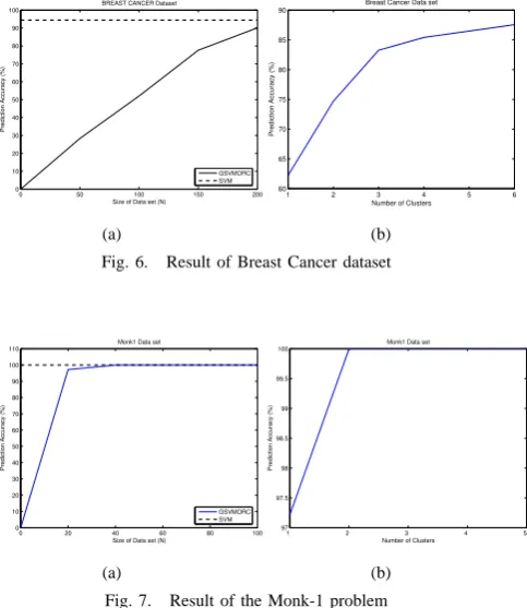
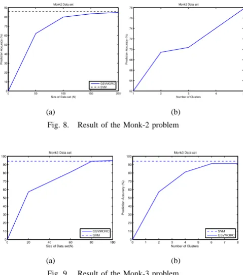
unseen cases according to a test set. The results show that when the data size increases, the accuracy of the rules increases, converging to that of the SVM as illustrated in the following Figures. For example, for the Iris dataset (see Figure 5(a)), whenNequals30, the accuracy is only77.33%. However,84.67%is achieved whenN equals100. It finally reaches 89.33% at N = 300, which is a value near to the accuracy of SVM. The same behavior is verified for the breast cancer dataset (see Figure 6(a)). When N equals50, the accuracy is only around 60%. Although the rate of the increase reduces, it still causes the accuracy result to finally reach 90.14% at N = 200. While for Monk’s problem (the results are shown in Figure 7(a), 8(a) and 9(a) , when N reaches100, GSVMORC achieves100%accuracy for Monk-1. For Monk-2, GSVMORC obtains 84.8% for a 200-size training set compared with the 85.7% accuracy classified by the SVM network. GSVMORC also achieves an average

95% correctness for a 100-size training set in the case of the Monk-3 problem, while the SVM obtains around 94% accuracy.

Figure 5(b), 6(b), 7(b), 8(b), 9(b) show that when the number of clusters increases, the accuracy increases as well. As an example, in the Iris dataset, GSVMORC classifies only

56% instances correctly when the cluster number is one.

0 50 100 150 200 250 300 0

10 20 30 40 50 60 70 80 90 100

Size of Data set (N)

Prediction Accuracy (%)

IRIS Data set

GSVMORC SVM

(a)

1 2 3 4 5 6 55

60 65 70 75 80 85

Number of Cluster

Prediction Accuracy (%)

IRIS Data set

(b)

Fig. 5. Result of Iris dataset

But it predicts 84% instances correctly when the number of clusters goes to six. It is interesting to note that the value of 84%, closest to the SVM accuracy of 89.33%, is obtained when the training set contains300instances and has one cluster for each class. The same convergence movement occurs for the Breast Cancer dataset. An accuracy of only

62.23% is obtained when each class has one cluster, but 87.55% of instances are predicted correctly when the number of clusters goes to six. For the Monk’s problem, the accuracy is only97%,62%and58%respectively for 1, Monk-2 and Monk-3, when the number of cluster is one. However, the accuracy increases to100%for Monk-1,78%for Monk-2 and90%for Monk-3, when the number of clusters increases to5. This is why we have chosen to use the stopping criterion of Section 3 to find an appropriate cluster value.

0 50 100 150 200 0

10 20 30 40 50 60 70 80 90 100

Size of Data set (N)

Prediction Accuracy (%)

BREAST CANCER Dataset

GSVMORC SVM

(a)

1 2 3 4 5 6 60

65 70 75 80 85 90

Number of Clusters

Prediction Accuracy (%)

Breast Cancer Data set

(b)

Fig. 6. Result of Breast Cancer dataset

0 20 40 60 80 100 0

10 20 30 40 50 60 70 80 90 100

110 Monk1 Data set

Size of Data set (N)

Prediction Accuracy (%)

GSVMORC SVM

(a)

1 2 3 4 5 97

97.5 98 98.5 99 99.5

100 Monk1 Data set

Number of Clusters

Prediction Accuracy (%)

(b)

Fig. 7. Result of the Monk-1 problem

Fidelity measures how close the rules are to the actual

0 50 100 150 200 0

10 20 30 40 50 60 70 80 90

Size of Data set (N)

Prediction Accuracy (%)

Monk2 Data set

GSVMORC SVM

(a)

1 2 3 4 5 62

64 66 68 70 72 74 76 78

Number of Clusters

Prediction Accuracy (%)

Monk2 Data set

(b)

Fig. 8. Result of the Monk-2 problem

0 20 40 60 80 1000 0

10 20 30 40 50 60 70 80 90 100

Size of Data set(N)

Prediction Accuracy (%)

Monk3 Data set

GSVMORC SVM

(a)

0 1 2 3 4 5 6 7 8 0

10 20 30 40 50 60 70 80 90 100

Number of Clusters

Prediction Accuracy (%)

Monk3 Data set

SVM GSVMORC

(b)

Fig. 9. Result of the Monk-3 problem

problems has been 100%. Monk-2 and Monk-3 obtained

99.12% and98.5%fidelity.

Comprehensibilitymeasures the number of rules and the

number of conditions per rule. The following is an example of the extracted rules on the Iris dataset. GSVMORC obtains on average ten rules for each class, with four conditions per rule.

sepal length= [4.3,6.6]Vsepal width= [2.0,4.0]Vpetal

length= [2.7,5.0]Vpetal width= [0.4,1.7]→Iris

Versicolour

The rule above correctly predicts45 out of150instances in the data set. Overall, 93% training and test examples in the Iris data set are predicted correctly.

The following is an example of the extracted rules on Breast Cancer problem. GSVMORC obtained on average26 rules for class 1and81rules for class −1, with an average

7.2 conditions per rule. The final rule set classifies 90.14% of the test cases and 93% of the whole data set correctly. a3= [4,9]

V

a5= [3,9]

V

a6= [10,10]

V

a7= [5,9]→ −1 For Monk-1, GSVMORC obtained four rules for all classes. On average, each rule has 2.37 conditions. This is from the100synthetic training instances, which cover100%

of the test cases. For Monk-2, around38rules were extracted, with around 4.1 conditions per rule for class1. For class 0,

24 rules with 5.8 conditions per rule were extracted. For Monk-3,11rules were extracted, with around3.4conditions per rule for class 1, while 6 rules with 2.7 conditions per rule were extracted for class 0 (for example a1 = 1

V

a2 = 1 → class = 1; in this case, a1 = 1 denotes that a1 istrue).

Discussion and Comparison with Related Work

We have shown how rules can be extracted from SVMs without needing to make many assumptions about the ar-chitecture, initial knowledge and training data set. We have also demonstrated that GSVMORC is able to approximate and simulate the behavior of SVM networks correctly.

The accuracy and the fidelity of our algorithm are better than those obtained by the SVM rule extraction approach proposed in [19], which is an important work on rule extraction from SVMs. GSVMORC obtains 100%accuracy for Monk-1, while the SVM+prototype [8] predicts only

59.49%of instances correctly in the test set. Compared with the 63.19% test-set performance by the rule base and the

82.2%SVM classification rate, GSVMORC achieves84.8%

accuracy on the test set while the classification of SVM is 85.7%. GSVMORC also obtains 100% fidelity, but the SVM+prototype has just 92.59% and 75.95% agreement with SVM networks in the respective data sets. (Note that the performance measures for the SVM+prototype and other techniques originate from published papers and not our own experiments [8].)

In the Iris problem, the SVM+prototype [19] reports an accuracy rate of 71% for interval rules and a fidelity rate of 97.33% compared with the 96% accuracy of RBF SVM networks [16]. Our algorithm achieves a maximum fidelity rate (100%) with a far higher accuracy (89.33%), while SVM accuracy is 91.33%.

In the Breast Cancer problem, the ExtractRules-PCM ap-proach of [6] achieves an average accuracy of98%compared with an SVM accuracy of 95%. In contrast, our extraction algorithm shows high agreement between the rules and the SVM. A good fidelity indicates that the rule extraction method mimics the behavior of SVM networks, and a better understanding of the learning process is therefore obtainable. In the Breast Cancer problem, the eclectic approach of [15] achieved82%accuracy compared with an SVM accuracy of

95%. Our approach performs better than that approach. It achieves 89% accuracy which is more closer to the SVM accuracy (94%).

In RuleExSVM [23], another vital algorithm for SVM rule extraction, rules are extracted based on the SVM clas-sification boundary and support vectors. RuleExSVM has high rule accuracy and fidelity in the Iris and Breast Cancer problems. For example, for the Iris problem, RuleExSVM achieves98%relative to the97.5%of the SVM classification results, and in the Breast Cancer domain, 97.8% accuracy is obtained. The fidelity levels of these two domains range from 99.18% to99.27%. However, RuleExSVM constructs the rules largely depending chiefly on the training samples and support vectors. It is difficult to apply to networks other than SVM networks. On the other hand, GSVMORC has a high level of generality in a wide array of networks.

NeuroRule relies on special training procedures that facilitate

the extraction of the rules. GSVMORC, on the other hand, is architecture-independent and has no special training require-ments. It offers the highest fidelity rate and an interesting convergence property, as illustrated in the figures above.

VI. CONCLUSION ANDFUTUREWORK

We have presented an effective algorithm for extracting rules from SVMs so that results can be interpreted by humans more easily. A key feature of the extraction algorithm is the idea of trying to search for optimal rules with the use of expanding hypercubes, which characterize rules as constraints on a given classification. The main advantages of our approach are that we use synthetic training examples to extract accurate rules, and treat the SVM as an oracle so that the extraction does not depend on specific training requirements or given training data sets. Empirical results on real-world data sets indicate that the extraction method is correct, as it seems to converge to the true accuracy of the SVM as the number of training data increases and 100% fidelity rates are obtained in every experiment. In future work, we may consider using different shapes than hypercubes for the extraction of rules and compare results and further improve the comprehensibility of the extracted rules.

Support Vector Machines have been shown to provide ex-cellent generalization results and better classification results than parametric methods or neural networks as a learning system in many application domains. In order to develop further the study of the area, we need to understand why this is so. Rule extraction offers a way of doing this by integrating the statistical nature of learning with the logical nature of symbolic artificial intelligence [20].

REFERENCES

[1] Charles. A and Dennis. J. E. Analysis of generalized pattern searches.

SIAM Journal on Optimization, 13(3):889–903, 2003.

[2] Garcez. A. A, Broda. K, and Gabbay. D. Symbolic knowledge extraction from trained neural networks: a sound approach. Artificial

Intelligence, 125(1 - 2):155 – 207, January 2001.

[3] Karaivanova. A, Dimov. I, and Ivanovska. S. A quasi-monte carlo method for integration with improved convergence. In LSSC ’01:

Proceedings of the Third International Conference on Large-Scale Scientific Computing-Revised Papers, pages 158–165, London, UK,

2001. Springer-Verlag.

[4] Thrun. S. B. Extracting provably correct rules from artificial neural networks. Technical report, Institut f¨ur Informatik III, Universit¨at Bonn, 1993.

[5] Pop. E, Hayward. R, and Diederich. J. Ruleneg: Extracting rules from a trained ann by stepwise negation. Technical report, December 1994. [6] Fung. G, Sandilya. S, and Rao. B. R. Rule generation from linear

support vector machines. KDD’05, pages 32 – 40, 2005.

[7] Morohosi. H and Fushimi. M. A practical approach to the error estimation of quasi-monte carlo integration. In Niederreiter. H and Spanier. J, editors, Monte Carol and Quasi-Monte Carlo Methods, pages 377–390, Berlin, 1998. Springer.

[8] N´u˜nez. H, Cecilio Angulo, and Andreu Catal`a. Hybrid architecture based on support vector machines. In Proceedings of International

Work Conference on Artificial Neural Networks, pages 646–653, 2003.

[9] Platt. J, Cristianini. N, and Shawe-Taylor. J. Large margin dags for multiclass classification. Advances in Neural Information Processing

Systems, 12:547–553, 2000.

[10] Platt. C. J. Sequential minimal optimization: A fast algorithm for training support vector machines. Technical Report MSR-TR-98-14, Microsoft Research, April 1998.

[11] Saito. K and Nakano. R. Law discovery using neural networks.

Proceeding NIPS’96 Rule Extraction From Trained Neural Networks Workshop, pages 62 – 69, 1996.

[12] Craven. W. M and Shavlik. J. W. Using sampling and queries to extract rules from trained neural networks. In International Conference on

Machine Learning, pages 37–45, 1994.

[13] Craven. W. M and Shavlik. J. W. Extracting tree-structured represen-tations of trained networks. In David S. Touretzky, Michael C. Mozer, and Michael E. Hasselmo, editors, Advances in Neural Information

Processing Systems, volume 8, pages 24–30. The MIT Press, 1996.

[14] Fu. L. M. Rule learning by searching on adapted nets. Proceedings

of the Ninth National Conference on Artificial Intelligence (Anaheim CA), pages 590–595, 1991.

[15] Barakat. N and Diederich. J. Eclectic rule extraction from support vector machines. International Journal of Computational Intelligence, 2(1):59 – 62, 2005.

[16] N´u nez. H, Angulo. C, and Catal`a. Rule based learning systems for support vector machines. Neural Processing Letters, 24(1):1–18, August 2006.

[17] Filer. R, Sethi. I, and Austin. J. A comparison between two rule extraction methods for continuous input data. Proceeding NIPS’97

Rule Extraction From Trained Artificial Neural Networks Workshop,

pages 38 – 45, 1994.

[18] Setiono. R. Extracting rules from neural networks by pruning and hidden unit splitting. Neural Computation, 9:205 – 225, 1997. [19] N˜u¨nez. N, Angulo. C, and Catal´a. A. Rule extraction from support

vector machines. Proceeding of European Symposium on Artificial

Neural Networks Bruges(Belgium), pages 107 – 112, 2003.

[20] Leslie G. V. Three problems in computer science. J. ACM, 50(1):96– 99, 2003.

[21] Vapnik. N. V. Statistical learning theory. John Wiley and Sons, INC, 1998.

[22] Morokoff. J. W and Caflisch. R. E. Quasi-Monte Carlo integration. J.

Comp. Phys., 122:218–230, 1995.

[23] Fu. X-J, Ong. C-J, Keerthi. S, Gih G-H, and Goh L-P. Extracting the knowledge embedded in support vector machines. volume 1, pages 291–296, 2004.