Load Balancing in Distributed Systems using
Diffusion Technique
P. Neelakantan
Department of CSE, SVUCE, Tirupati, India
ABSTRACT
The purpose of load balancing algorithm is to distribute the excess load from heavily loaded nodes to underloaded nodes. A new dynamic load balancing algorithm is proposed based on diffusion approach (DDD) for homogeneous systems where the processing capacities of all nodes in the system are equal. The proposed algorithm works iteratively to balance the load among the nodes in a system. The dynamic distributed diffusion algorithm has been developed for coarse and large granularity applications, where the load shall be treated as an Integer quantity. The functioning of the proposed algorithm is demonstrated by using a random graph & simulation has shown the proposed algorithm performs better in terms of time taken to balance the load, minimizing the load variance among the nodes and maximizing the throughput.
Keywords
Load balancing, diffusion
1.
INTRODUCTION
A well known and popular load balancing approach first introduced by Cybenko and Boillat [1][2] is diffusion load balancing. The algorithm works iteratively to balance the load among the nodes in a system. The idea behind this algorithm is in each round, the overloaded node exchanges its excess load with all neighbors individually. The advantage of diffusion algorithm lies in the collection of information from the nodes in a system. The information policies will have higher impact on earlier completion of load balancing algorithm.
The diffusion algorithm [3, 4, 5] collect information from a group of nodes which is referred to as a domain. The algorithm tries to balance the loads in each domain, such that excess load will be transferred to the under loaded node in their domain thus reducing communication overhead. When loads are to be transferred to the large radii node in a system it puts more communication overhead which forfeits the advantages of load balancing algorithm. The objective of the diffusion load balancing algorithm in both static load situations and in dynamic load situations is to keep the nodes to contain an equal number of loads. To do this, the loads are distributed evenly among the nodes as quickly as possible. Much work has been done under the assumption that every edge is only allowed to forward one load unit per round [6, 7, 8, 9] or a constant number of loads can be passed by each node [10, 11].
In a simple diffusion algorithm, if the neighboring nodes of any have the load value smaller than underlying then those neighbors are referred as underloaded loaded nodes. Once underloaded neighbours are determined, the underlying node will measure the load difference between itself and each one of its neighbours. Then, a fixed portion of
the excess load is sent to each one of the under loaded neighbours. This strategy, as well as other strategies from the literature based on this, [5][12][13] is originally conceived under the assumption that load can be divided arbitrarily ,i.e., the load is treated as a non-negative real quantity. The load is treated as integer quantity in medium and large grain parallelism (back-track searches, branch-and-bound optimizations, theorem proving, interpretation of PROLOG programs, adaptive refinement techniques for solving PDEs, and ray tracing )which are more realistic assumption and common in practical parallel computing environments as carried out in [14] [15[11]]. A relevant strategy in this area is the SID (Sender Initiated Diffusion) algorithm [12]. Luling and Monien [13] devised a distributed load balancing algorithm for a grid with load index defined as a summation of service times of jobs currently running in a node but does not consider the effects of communication latency. Liu et al. [19] used an agent based system, which migrates the excess workload from the heavily loaded nodes to the lightly loaded nodes, and they assumed the nodes in the system are homogeneous. Acker et al., [20] proposed a new decentralized dynamic diffusion algorithm that is capable of dynamically adapting to changing operating parameters. The devised load balancing algorithm runs on every node is decentralized and dynamic. It handles the nodes in the systems that are heterogeneous in terms of node processing capacity, architecture and network speed.
2.
NOTATIONS & ASSUMPTIONS
Consider a distributed system with nodes represented as an undirected graph G , where a set of nodes and set of edges connecting the nodes. The set of nodes that have direct links with is represented by called neighbor nodes [6][8][11].
Notations:
N: Number of nodes in a distributed system
V: set of nodes in a distributed system N=|V| : Load of node i at time t i
Domain of node i at time t = : Load of node that belongs to domain of node at time t
: Average load of the domain of node i given by
: Average System load at time t
Variance of system,
: Excess load of node i at time t
Maximum load of node in the domain of node i
: Minimum load of node in the domain of node i
: Apportion of the load sent to the deficit neighbor j in the domain of node i
: Fine load distribution by node i
It is assumed that a distributed system consists of identical high performance nodes (homogeneous system) connected by a set of high bandwidth communication links in order to provide a powerful computing platform to execute computationally intensive parallel and distributed applications [11].
It has been assumed a distributed system consists of independent parallel jobs [5] [6] [7] where they can be executed at any time, in any order and at any node. It is assumed that the jobs have varied service times and are modeled as a uniform distribution. The arrival of the jobs is a Poisson distribution.
3.
MATHEMATICAL MODEL
Let is the load value of node in a system of N nodes at given time instant t and the load values among the nodes in the system are represented by using load vector . The load values of a node can be real or non negative integer values depending on the granularity of the application. Let the load value of every node in a system is represented as an integer quantity. When the load is represented as an integer quantity the maximum load difference in the system between any two nodes is to be 0 or 1.
Let the load balancing algorithm is initiated at time t and it takes some time t1 where t1>t to balance the load among the nodes. Let the average system load at time t is given by
(3.1)
Since load balancing algorithms are load conservative, i.e., they do not neither create nor destroy load but only move it around the system such that load values of individual nodes changes due to load balancing actions .In static load situations, the value of does not change over time. Thus, it is given by
The imbalance of the system load at time t is measured with a synthetic indicator, the variance of the load of the nodes, i.e., their quadratic deviation from .
(3.2)
If variance among the system is minimized, each node in the system contain equal loads to process so as to minimize the response time of the system.
Theorem:
The execution of a diffusive load balancing policy nullifies any load imbalance in a system[6][11], i.e.,
(3.3)
Lemma: If the variance among the nodes in a domain D is decreased by exchanging the loads only among the nodes in that domain by applying load balancing algorithm then the global variance of the system can also be decreased.
Proof:
Let us multiply the expression (3.2) by N and for the sake of simplicity exclude the right hand side value N which is multiplied with .The variance at time t can then be expressed as:
=
= (3.4) After initiating a load balancing activity at time t within a domain of nodes, the variance at time can be expressed as:
=
= (3.5)
The variation of the variance can be expressed as =
(3.6)
Let us consider the load balancing activity takes place in a domain and not in the in other domains . The load balancing algorithm exchanges load in the nodes that are present in a domain (by indicating , the set of nodes not belonging to the domain and by the number of nodes involved in load balancing)
=
, =
The equation (3.6) can also be rewritten as follows =
(3.7)
By adding and subtracting the terms , in equation (3.7)
= + ( (3.8)
The above equation can be expressed as
(3.9)
In other words, the variation of the global variance can be expressed as the variation of the variance in the sub systems identified by and . The load of the nodes of has not changed, i.e.,
=0 (3.10)
Consequently, if the local action in D decreases the local variance
4.
PROPOSED METHOD
In a distributed system, the nodes exchange their load information at periodic intervals of time called information exchange interval . The information exchange consists of load information of a node and the instant at which this information exchange takes place is called an information exchange epoch. In order to reduce the communication overhead, the information exchange is restricted only to the neighboring nodes.
Each node i receives a load information message from its neighbors which is kept in the node i memory. Due to communication delays induced by the network, each node i will have an estimate of the neighbor nodes load, because within the communication delay d some load may be added to the node j or removed from the node j. The load information from node j to node i is represented where is a certain time instant satisfying
. The node i, as =0 (delay is zero for the node i)
will have exact information about its load.
A set of time instants is associated with each node for doing load balancing. At a given time instant, the node i executes the load balancing algorithm by comparing its load with the estimated load of its neighbors that are stored in the node i local memory during status exchange epoch. In order to analyze the DDD behavior, the variable t is discriminated by assuming the values t=0, 1, 2….
When the loads among the nodes are distributed randomly, a single iteration of the proposed load balancing algorithm consists of two procedures: procedure LB and procedure AccurateLB. In procedure LB, when the load of the node is greater than the average load of the domain of the node i, then that node is said to be an overloaded node, so it sends its excess load to the under load neighbors.
In the procedure AccurateLB of DDD, the node that initiated the load-balancing algorithm checks its underlying domain for balanced state. The domain attains balanced state if the load difference between two nodes in it is not greater than 1. If it is not balanced, a node that initiated the load balancing algorithm balances its domain in a refined way by sending messages to the overloaded nodes in its domain to distribute the loads to the under loaded neighbors
The node i compute the load average of its domain by taking the load information of the neighbors kept in the memory which is rounded to the nearest lowest integer value, which is given by
(4.1)
After computing the load average, it evaluates the relative load weight to detect whether it is an overloaded node or under loaded node. For this purpose it uses the below formula
(4. 2)
From equation (2) If the value >0 indicates node i is overloaded and it has to send its excess load to one of its deficient neighbors. The value <0 indicates that the node is underloaded and there no need to transfer the load and hence no need to invoke the load
balancing algorithm. Depending on the value of ) the load balancing algorithm is initiated by the node i
4.1.1 Load transfer calculation
Once the node i determines that it is having an excess load, it has to distribute its excess load to the deficient neighbors. The node i form two sets and depending on the excess and deficit load values. Nodes having the deficit loads form the Active set which is denoted by and nodes having the excess loads form the set After forming the two sets, for each deficit neighbor in set , load deficit for an individual node is stored which is given by
Activei (t) = where
Sendi(t) = where k
=
The total deficit of the domain of node is calculated by using the formula:
= (4. 3)
After determining the total deficit load, the node i proceed to determine how much portion of its excess load is to be sent for each deficit neighbor by having the below formula
(4. 4)
4.1.2 Accurate Load Movements
The procedure AccurateLB is used by node i to check its domain for accurate balance. To do this, some additional parameters are required to probe for unbalanced domains. These parameters will do accurate load movements to balance the domain and hence to decrease the variance of the domain. The additional parameters introduced in the algorithm are:
A node that contains a maximum load value in the domain of :
A node that contains a minimum load value in the domain of : {
To detect the imbalance in domain of , the above two parameters will be used .
4.1.3 Load adjustments between nodes
After detecting, the imbalance in the domain of , some units of load must be moved between the nodes to reduce the variance in the domain of . To do this the following steps must be accomplished.
Step 1: In general excess loads are kept in and deficit loads are kept in the set . When the load difference between the maximum loaded node in and minimum loaded node in is greater than 1 & all nodes in contains equal loads load refinement must be done such that all nodes in the domain must consist of nearly an equal amount of load.
contains load units greater than 1, some load units must be transferred. While transferring two constrains must be satisfied.
Constraint 1: The node in the set after sending its excess load units to one of the deficient neighbors in the set ,load value of the sender node must be equal or greater than one unit to the next higher load node in is compared to avoid job shuttle between the nodes. From this, it will be concluded that the largest node in remains as largest after sending units of load to least loaded deficit node in
Constraint 2: After receiving load units from the maximum loaded node in , the load value of the least loaded node in must be equal to the load value of the next least loaded node in . The above two constraints plays a key role in avoiding job thrashing effect.
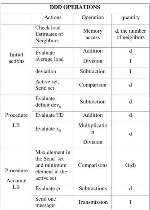
To analyze the time complexity of DDD algorithm, The single iteration of DDD in a node involves distinct operations depending on the phase or phase of the algorithm to be executed to distribute the load among the neighbors. The below pseudo code of the algorithm shows the organization of different blocks and table 1 shows the maximum number of operations required at each level( The number of neighboring nodes to node is denoted as d). By complete analysis, it shall be concluded that the time complexity of DDD is prevailed by the complexity of AccurateLB O(d).Hence it can be seen that the overall time complexity of the DDD is low when compared to the load balancing algorithms discussed in the literature survey.
Algorithm DDD
At each node i=1, 2…N
Compute ;
Find = where
Find = where
Compute (t) = ;
If ( (t)>0) call procedure LB;
Choose an index k & a ;
= ;
= ;
While ( >1)
Compute ;
If ( 0) exit;
Else
Call procedure AccurateLB;
Choose an index k & a ;
= ;
= ;
End while
End DDD
Procedure LB
For each jActivei
Compute (t);
End For
Compute ;
For each jActivei
Compute
;
Transfer units to node j from node i;
End For
End LB
Procedure AccurateLB
If (i
Node i sends message to k to transfer load unit to a and the load at k is reduced by one unit.
Else
Node i transfer load unit to a and the load at i is reduced by one unit.
End AccurateLB
DDD OPERATIONS
Actions Operation quantity
Initial actions
Check load Estimates of Neighbors
Memory access
d, the number of neighbors
Evaluate average load
Addition
Division
d
1
deviation Subtraction 1
Active set,
Send set Comparison d
Procedure
LB
Evaluate deficit devij
Subtraction d
Evaluate TD Addition d
Evaluate xij
Multiplicatio n
Division
d
Procedure
Accurate LB
Max element in the Send set and minimum element in the active set
Comparisons O(d)
Evaluate Subtractions d
Send one
[image:4.595.309.551.380.718.2]message Transmission 1
4.2 CONVERGENCE OF THE PROPOSED ALGORITHM
To demonstrate DDD convergence, partially asynchronous assumption introduced by authors in [11][6][12]. The asynchronous algorithms are divided into two classes: totally asynchronous and partially asynchronous. Total asynchronous algorithms can tolerate large communication and computation delays but partially asynchronous algorithms require an upper bound on communication and computation delays to work correctly. This upper bound is denoted by U, which is applied to realistic load model assumed by DDD. The formal description of this assumption is given below. The time complexity of the proposed algorithm is O(d).
Assumption 1: Let us denote an upper bound U such that
a) For each node and for every ,
b) For each node , for every and for every
c) Node sends the load to node j at time t, will be received by the node before time t+U
d) Node sends the instruction message to node j at time t, is received by the node before time t+U
Part (a) of this assumption asserts that the load balancing step is performed by each node during time interval of length U. (b) states that load information of neighboring nodes kept by any node in a given time t are obtained at any time between t-U and t; (c) & (d) asserts that the instruction messages and load messages sent by node i to node j will not be delayed more than U time units.
To Prove DDD converge under assumption 1, two definitions and two lemmas are to be introduced.
Definition 1: is the minimum load value in a system during the time interval t-3U to t.
Definition2: = , where is the minimum load value that occupies k-st place if the loads are sorted in non decreasing sequence during the time interval t-3U to t.
Lemma 1: The sequence of loads ( , the time is increasing and upper bounded. There exist a time t1 such that
I. =
II. ,
=
From Lemma1 it has been observed that at time , the load value of all nodes become stable and no node would send or receive the load from its neighbors by executing the DDD algorithm.
Proof: Let a node i V and a time It is to be proven that Li(t+1)
If then is not having the excess load, so it does not trigger the load balancing algorithm, instead it receives the load from the overloaded neighbors as a part of load balancing process which is initiated by some overloaded neighbor which
is present in its domain. Thus
If , the node i has invoked the load balancing algorithm, where two different cases shall be found depending on which procedure in DDD is invoked in making the accurate load movements between the nodes.
Case 1: When there are no load movements has been generated by AccurateLB( , then there exits two different situations.
Situation 1: Node is an under loaded node ( (t) ≤ 0). Then it will not send any load to its neighbors such that so .
Situation 2: Node i is an overloaded node ( (t) . Then it will execute the procedure LB to migrate some load units to the deficient neighbors which is given by
= + .
Here is the average load of the domain between the time interval t- 3U to t, so it is clear that is greater than . Hence
Case 2: By applying the procedure AccurateLB, some load units move among the nodes ( . It may be possible that an overloaded node does not transfer any load by using the procedure LB, but still there is chance to transfer some load units to the deficient neighbors in a more refined way to reduce the load variance in the system by calling the procedure AccurateLB. This happens in two different situations.
When the difference between the loads of first nodes in Activei and Sendi is greater than 1, i.e., = ( and the node i is having the maximum load in its domain then
is sent to the least loaded neighbors.
Thus =
When the difference between the loads of first node in Activei and Sendi is greater than 1, i.e., = (
, node i is not having the maximum load in its domain but belongs to sendi , but there exists some node k with maximum load in domain of node i such that it sends an instruction message to k to send
-
is sent to the least loaded neighbors such that at some time , the difference between where So, it shall be concluded that .
Hence for all the cases it has been shown that and . So minimum load at t+1 is greater than minimum load at t which is given by
integer such that So part (I) of lemma is proved for any time .
To prove part (II) of Lemma1, Let is the set of nodes with load value less than or equal to the average load of the system at time t and it will be seen that i.e., the sequence of sets of nodes with minimum load is a decreasing sequence beyond .
Let and . It will be seen that , i.e., if node is not a node with minimum load value at time t then it will be never be a node having a minimum load value at time t+1.
If , then it has been proven that
so
If , some different cases can be found:
Case 1: If then, as it has been observed . So .
Case 2: If and node i is an underloaded node ( then it has been seen that thus
Case 3: If and node is an overloaded node ( then it has been seen that
and
So it can be concluded that
Since is a finite set, there exists an integer such that
Note that if has the minimum load value at time then . Because it is an under loaded node it does not send any load such that and does not receive any load from neighbors.
Since both (I) & (II) of Lemma 1 is proved, hence Lemma 1 is proved
5.
SIMULATION
The objective for load balancing is obtain a uniform response time throughout the system. For evaluating the performance of the load balancing algorithms M/D/1 Queuing model is used. The expected response time of a node is modeled as a M/D/1 queue depends on the mean and standard deviation of service times and on the average inter-arrival time. The D in this model stands for constant service time. The inter arrival time of requests on a node has a mean value of which follows a Poisson distribution
5.1 INFLUENCE OF NODE SIZE ON EXECUTION TIME OF AN ALGORITHM
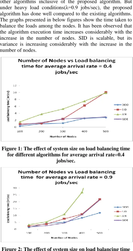
[image:6.595.316.543.174.601.2]To test the influence of node size on the execution time of an algorithm, the loads are varied from light load situations to high load situations by adjusting the parameter λ. The sizes of the nodes are varied from 100 nodes to 500 nodes to test the scalability of the algorithms. It has been observed under light load conditions (λ=0.1 jobs/sec), the GDE algorithm has been performing well when compared to the other algorithms inclusive of the proposed algorithm. But under heavy load conditions(λ=0.9 jobs/sec), the proposed algorithm has done well compared to the existing algorithms. The graphs presented in below figures show the time taken to balance the loads among the nodes. It has been observed that the algorithm execution time increases considerably with the increase in the number of nodes. SID is scalable, but its variance is increasing considerably with the increase in the number of nodes.
Figure 1: The effect of system size on load balancing time for different algorithms for average arrival rate=0.4
jobs/sec.
Figure 2: The effect of system size on load balancing time for different algorithms for average arrival rate=0.9
jobs/sec.
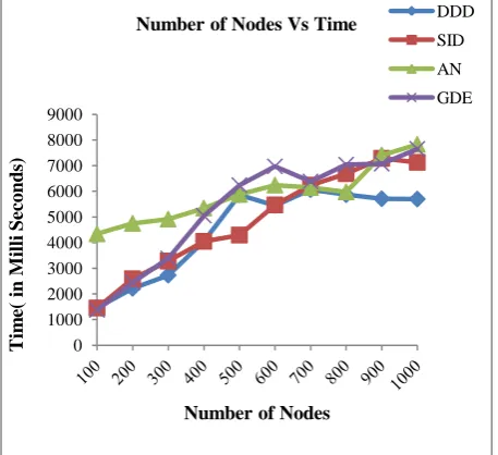
5.2 EFFECT OF NODE SIZE ON VARIANCE
[image:6.595.317.543.272.415.2]present and the variance among the nodes is decreasing constantly as the load balancing algorithm progresses over time.
Figure 3 shows the time taken for different algorithms to reduce variance among the nodes in the system when the
average arrival rate λ=10 jobs/sec.
5.3 EFFECT OF ARRIVAL RATE ON THROUGHPUT
In this simulation, the nodes are generated randomly with reachability of every node in the system. The edges connecting the nodes are generated in such a way that the graph is a spanning tree. In low load conditions, the GDE has performed well in executing the more number of jobs per unit time. Even though AN & the proposed algorithm DDD has attained low variance they have taken more time to reduce the variance among the nodes in the system thus resulting in low throughput when compared to GDE. But in moderate and heavy load conditions, the proposed algorithm has done well when compared to the other algorithms. The GDE algorithm has occupied next to the DDD algorithm.
6.
REFERENCES
[1] J.E. Boillat, Load Balancing and Poisson Equation in a Graph, Concurrency: Practice and Experience, Vol. 2(4), December 1990, pp. 289-313.
[2] G.Cybenko, Load balancing for distributed memory multiprocessors. Journal of Parallel and Distributed Computing, 7:279-301, 1989.
[3] Rupali Bhardwaj, V.S.Dixit, Anil Kr.Upadhyay. A Propound Method for Agent Based Dynamic Load Balancing Algorithm For Heterogeneous P2P Systems in International Conference on Intelligent Agent and Multi-Agent Systems, 2009.
[4] F.M. auf der Heide, B. Oesterdiekhoff, and R. Wanka. Strongly adaptive token distribution. Algorithmica 15 (1996), pp. 413–427.
[5] Berenbrink, P. and Friedetzky, T. and Martin, R. (2005) ’Dynamic diffusion load balancing.’, in Automata, languages and programming : 32nd International Colloquium, ICALP 2005, 11-15 July 2005, Lisbon, Portugal ; proceedings. Berlin: Springer, pp. 1386-1398.
[6] Cortés, A., Ripoll, A., Cedó, F., Senar, M. A., and Luque, E. 2002. An asynchronous and iterative load balancing algorithm for discrete load model. J. Parallel Distrib. Comput. 62, 12 (Dec. 2002), 1729-1746.
[7] Y.F. Hu, R.J. Blake, An Improved diffusion algorithm for dynamic load balancing, Parallel Computing 25(1999), pp. 417-444.
[8] E. Luque, A.Ripoll, A.Cortes and T. Margalef, A Distributed Diffusion method for dynamic load balancing on parallel computers,1995.
[9] Tina A. Murphy and John G. Vaughan, On the Relative Performance of Diffusion and Dimension Exchange Load Balancing in Hypercubes, Procc .of the Fifth Euromicro Workshop on Parallel and Distributed Processing, PDP’97, January 1997, pp. 29-34.
[10]P. Berenbrink, T. Friedetzky, and Z. Hu. A new analytical method for parallel, diffusion-type load balancing. J. Parallel Distrib. Comput., 69(1):54–61, 2009
[11]F. Cedo, A. Cortes, A. Ripoll, M. A. Senar, and E. Luque. The convergence of realistic distributed loadbalancing algorithms. Theor. Comp. Sys., 41(4):609– 618, 2007.
[12]D.P. Bertsekas and J. Tsitsiklis, Parallel and Distributed Computation: Numerical Methods,Prentice-Hall, Englewood Cliffs, NJ, 1989.
[13]Liu, J., Jin, X. and Wang, Y. 2005. Agent-Based Load Balancing on Homogeneous Minigrids: Macroscopic Modeling and Characterization, IEEE Transactions on Parallel and Distributed Systems, 586-594.
[14]Raghu Subramain, Issac D. Scherson, An Analysis of Diffusive Load-Balancing. In Proceedings of 6th ACM Symposiummon Parallel Algorithms and Architectures, 1994.
[15]T. Friedrich and T. Sauerwald, "Near-perfect load balancing by randomized rounding", in Proc. STOC, 2009, pp.121-130.
0 1000 2000 3000 4000 5000 6000 7000 8000 9000
Tim
e(
in
M
ill
i
Sec
o
n
d
s)
Number of Nodes
Number of Nodes Vs Time DDD SID
AN
GDE
0 0.1 0.2 0.3 0.4 0.5 0.6 0.7 0.8
0.1 0.2 0.3 0.4 0.5 0.6 0.7 0.8 0.9
Th
ro
u
gh
p
u
t(
job
s/se
c)
Arrival rate(jobs/sec)
Arrival rate vs Throughput for the node size=500
DDD
SID
AN
[16]Marc H. Willebeek-LeMair, Anthony P. Reeves, Strategies for Dynamic Load Balancing on Highly Parallel Computers, IEEE Transaction on Parallel and Distributed Systems, vol 4, No 9, September 1993, pp.979-993.
[17]Qiao, Y. and Bochmann, G. v. 2009. A Diffusive Load Balancing Scheme for Clustered Peer-toPeer Systems. In Proceedings of 15th ICPADS. IEEE Computer Society, 842-847
[18]S. Muthukrishnan, B. Ghosh, and M. Schultz. First and second-order diffusive methods for rapid,
coarse,distributed load balancing. Theory of Computing Systems, 31(4):331–354, 1998
[19]Luling, R., Monien, B. 1993. A Dynamic Distributed Load Balancing Algorithm with Provable Good Performance. Proc. of the 5th ACM Symposium on Parallel Algorithms and Architectures, 164-173