Load–Frequency Control Assessment using Restoration Index with Artificial Bee Colony Algorithm for Interconnected Power System with Disturbance Accommodation Controller

Load–Frequency Control Assessment using

Restoration Index with Artificial Bee Colony

Algorithm for Interconnected Power System with

Disturbance Accommodation Controller

R. Jayanthi

Department of Electrical Engineering Annamalai University

Annamalai Nagar- 608002 Tamil Nadu, India

I. A. Chidambaram

Department of Electrical Engineering Annamalai University

Annamalai Nagar- 608002 Tamil Nadu, India

ABSTRACT

Based on the concept of Modern Control theory, an optimal robust power system controller for power restoration problem using Disturbance Accommodation theory has been adopted in this paper. This proposed methodology is applied to a Two-Area Two-Unit thermal Reheat Interconnected Power System (TATURIPS) taking into account of Super Conducting Magnetic Energy Storage (SMES) device and Gas Turbine (GT) unit in either area to meet out the system uncertainties due to various disturbances. For Load-Frequency Control (LFC) a decentralized PI controller for each area and a centralized Disturbance Accommodation Controller (DAC) in TATURIPS co-ordinated with SMES and GT units as back-up energy suppliers have been implemented in this proposed methodology. Feasible Restoration Index (FRI) and Complete Restoration Index (CRI) are computed for various disturbances based on settling time of the output response of the system and the control input deviation. The decentralized controller is tuned using the Artificial Bee Colony (ABC) algorithm. With these two Restoration Indices obtained from the Intelligent Controller (IC) as well as DAC, the conditions required to be satisfied in ensuring the restoration of the power system are listed out and with proper implementation will result in high degree of reliability and stability of power supply reducing the frequency deviations to a greater extent and the settling time is also reduced to a minimum time span.

Keywords

Restoration Index, Disturbance Accommodation Controller, Settling Time, Proportional-Integral Controller, Artificial Bee Colony.

1.

INTRODUCTION

In the interconnected power systems there are number of control areas or units and each control area has to generate the required amount of power to satisfy the customer load requirements as well as it has to maintain the system frequency, tie-line power deviation, control input requirements within the scheduled levels. A high gain may deteriorate the system performance leading to instability of the system. Therefore, in order to maintain the load generations balance and the quality of power at requisite level an intelligent decentralized PI controller using Artificial Bee Colony (ABC) algorithm accompanied with a centralized DAC controller has been proposed to reduce the oscillations

due to frequency deviations and also to minimize the time span of settling time[1]. When an incident occurs on the system frequency within the stipulated limits is a major priority and if these limits are breached, then the magnitude of the excursion needs to be restricted and the frequency has to return within the limits as quick as possible. Therefore, based upon optimal control strategy an approach has been constructed which controls all the power generating stations. In the modern control theory concept the design of an intelligent decentralized controller in the system within the area is required where the local system variables are controlled. Due to the requirement of perfect model, which has to track the state variables and satisfy the system constraints, ABC tuned Proportional-Integral (PI) controller along with Disturbance Accommodation Controller with addition of a small capacity SMES unit and GT units to the system significantly improves the transients of frequency, tie-line power deviations and reduces the settling time span against load changes. SMES and GT units with a minimum capacity can be applied not only as a fast energy compensation device for large loads but also to damp out the frequency and tie-line power deviations, which makes it a cost-effective system. Moreover Gas Turbines become increasingly popular in different power systems due to their green house emission as well as higher efficiency especially when connected in a combined cycle setup [2, 3]. Various case studies has been analyzed for 1% and 4% disturbances and Restoration Indices are obtained from the simulation results and Restoration Indices, the required control efforts can be determined to provide a good control over the uncertain disturbances occurring in the system.

2.

MODELING OF THE TATURIPS

uncontrollable system variables, the controller design must be able to model their anticipated performances using a classical approach.

Fig 1: TATURIPS with SMES and GT units The generation changes must be made to match the load perturbation at the nominal conditions, if the normal state is to be maintained. The mismatch in the real power balance affects primarily the system frequency but leaves the bus voltage magnitude essentially unaffected. In a power system, it is desirable to achieve better frequency constancy than obtained by the speed governing system alone. This requires that each area should take care of its own load changes, such that schedule tie power can be maintained. A two-area interconnected system dynamic model in state variable form can be conveniently obtained from the transfer function model. The state variable equation of the minimum realization model of the „N‟ area interconnected power system is expressed as [4]

𝑋 = 𝐴𝑥 + 𝐵𝑢 + 𝜏𝑑 (1)

𝑌 = 𝐶𝑥 (2)

Where, the system state vector X consists of the following variables as

𝑥

= 𝐴𝐶𝐸1 𝑑𝑡, 𝐴𝐶𝐸2 𝑑𝑡, ∆𝐹1 ,∆𝑃𝑔1 , ∆𝑃𝑟1,∆𝑋𝑒1, ∆𝑃𝑡𝑖𝑒𝑙, ∆𝐹2, ∆𝑃𝑔2, ∆𝑃𝑟2,∆𝑋𝑒2 𝑇

System control input vector is 𝑢 =∆𝑃_∆𝑃𝑐1

𝑐2

System disturbance input vector is 𝑑 =∆𝑃_∆𝑃𝑑1

𝑑2

A is system matrix, B is the input distribution matrix and Γ disturbance distribution matrix,𝑥 is the state vector,𝑢 is the control vector and 𝑑 is the disturbance vector of load changes of appropriate dimensions. The typical values of system parameters for nominal operation condition are given in appendix. This study focuses on optimal tuning of controllers for LFC and tie-power control using settling time based optimization to ensure a better power system restoration assessment. On the other hand in this study the goals are to control the frequency and inter area tie-power with good oscillation damping using the modern control theory concept and also to obtain a good performance under all operating conditions with various loading conditions and finally to design a low-order controller for easy implementation. To achieve the above said conditions a Feasible Restoration Index (FRI) and Complete Restoration Index (CRI) based on the settling time has been formulated in this proposed methodology in TATURIPS with the SMES unit and GT unit in Area-1and

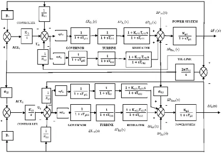
Area-2 respectively. Their Proportional (P) and Integral (I) gains has been optimized in addition with that of a Disturbance Accommodation Controller to achieve the improved restoration. Transfer function model of the two-area two-unit thermal reheat interconnected system used for implementation is as shown in figure 2.

2.1 Problem Formulation of TATURIPS

With DAC

The linear frequency control problem for a TATURIPS may be stated as follows, in which the N-area problem can be defined by [5]

𝑥 𝑡 = 𝐴 𝑡 𝑋 𝑡 + 𝐵 𝑡 𝑈 𝑡 + 𝐹 𝑡 𝑊 𝑡 (3)

𝑌 𝑡 = 𝐶 𝑡 𝑋 𝑡 (4)

Where 𝑋, 𝑈 and 𝑊 are state, control and disturbance vectors and 𝑌 is the system output. The TATURIPS is ideally defined by a set of state variables including the control input (speed changer position) and disturbance input (area load variation) in each area. As in this study the disturbances are treated as initial conditions on the system state variables, mathematically it can be modeled as a weighted linear combination of a set of known functions [6]

𝑊 𝑡 = 𝐶1𝑓1 𝑡 + 𝐶2𝑓2 𝑡 +, … . . , +𝐶𝑚𝑓𝑚 𝑡 (5)

Where the function 𝑓𝑖 𝑡 represent the various waveform

patterns that can be obtained from the daily load pattern and 𝐶𝑖 is piecewise random constant parameter. Therefore, the

overall power system disturbances for TATURIPS using DAC can be [5] modeled as

𝑤 = 𝑊 𝑧, 𝑡

𝑧 = 𝑍 𝑧, 𝑡 + 𝜎 𝑡 ; 𝑧 = (𝑧1, 𝑧2, … . , 𝑧𝜌) (6)

Which is the proposed mathematical model for disturbances having waveform structure recognized as the state-variable equation (1), where 𝜌-dimensional vector z(t) in (7) define the state of the disturbance which is considered to be a fictitious quantity. In particular, it is the value of the instantaneous state z(t) of an uncertain disturbance w(t), that contains all necessary information to make on-line decision of the control u at time t, even if the future disturbances are unknown quantities. Figure 3 shows the ithcontrol area diagram. Where the state variables containing the essential information about

the ith area can be defined as in (3).

Apart from the usual representation of the uncertain disturbances wi use is made of the waveform model (7). As referred from [5] a set of three basis functions𝑓1= 1, 𝑓2=

𝑡, 𝑓3= 𝑒−𝑎𝑡 is chosen to represent the actual load pattern

Fig 2: The TATURIPS

𝑊 𝑡 = 𝐶1+ 𝐶2𝑡 + 𝐶3𝑡𝑒−𝑎𝑡 (7)

The primary objective of the control U is to maintain the regulation of area frequency while simultaneously counteracting the system disturbances. In DAC, in particular the maximum absorbing mode of the critical state variable which is the frequency control as per the analysis using DAC can be used to design the controller that automatically uses the action of system disturbances to achieve an effective restoration of the electric power system.

Fig 3: Block diagram of ith control area

2.2 Application of DAC in TATURIPS

Single area representation of the Two-Area Two-Unit Reheat thermal Interconnected Power System is denoted by the system state and control variables as X1=Δf, X2=ΔP, X3=ΔXg, U=ΔPc .The system matrices A, B, C and F in this case can be obtained from the same as

𝐴=

𝑓∗ _{2𝐻 𝑓}∗ _{2𝐻 0}

0 −1 𝑇𝑡 1 𝑇𝑡

−1 𝑇 𝑅𝑔 0 −1 𝑇𝑔

; 𝐵= 0 0 1 𝑇𝑔

;

𝐶= 1, 0, 0 ; 𝐹= 𝑓∗ _2𝐻

0 0

(8)

To achieve the objective of control U, that is to maintain the frequency to the nominal value and tie-line power deviation close to zero by counteracting with the disturbances in the system one can choose to minimize the performance index of the form

𝑀𝑖𝑛 𝐽 𝑈; 𝑋0, 𝑡0, 𝑇 = 1₂𝑋𝑇 𝑇 𝑆𝑋(𝑇)

+1₂ 𝑋_𝑡𝑇 𝑇 𝑡 𝑄𝑋 𝑡 + 𝑈𝑇 𝑡 𝑅𝑈 𝑡 𝑑𝑡

0 (9)

2.3 Disturbance Absorption for a Critical

State Variable

In this paper for the Two-Area Two-Unit Reheat Interconnected Power System, the system frequency deviation is considered to be the prime factor of load changes and analysis has been carried out to minimize the disturbance effect to a maximum by absorbing the system frequency deviation to a maximum extent by considering the total effect of disturbances W(t) on just the system frequency deviation X1 which is nothing but the critical variable control problem. To absorb the disturbance effects on the area frequency DAC „critical variable‟ control action is considered. The differential equation governing X1= Δf alone can be obtained from state expressions, by repeated differentiation 𝑈𝑐 𝑡 is obtained,

which is designed to counteract the disturbance effects on X1 and simultaneously regulate X1 → 0..The total control U(t) can be expressed [3] by

𝑈 𝑡 = 𝐾𝑧𝑍 𝑡 + 𝐾𝑥𝑋(𝑡) (10)

𝑈 𝑡 = 𝐾𝑧 𝑍 (t)+ 𝐾𝑥𝑋 (t ) (11)

Where 𝑍 (t) and 𝑋 (t) are accurate estimates of Z(t) and X(t) which will be obtained from Y(t) on online, real-time state reconstructer.

2.4 SMES UNIT

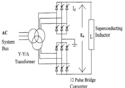
The Superconducting Magnetic Energy Storage (SMES) system is a fast acting device which can damp out these oscillations and help in reducing the frequency and tie-line Power deviations for better performance of system disturbances. It is designed to store electric energy in the low loss superconducting coil. Power can be absorbed or released from the coil according to the system requirement. A super conducting magnetic energy storage(SMES) is capable of controlling active and reactive power simultaneously and has been expected as one if the most effective stabilizers of power oscillations[7,8]. The schematic diagram in Fig.4 shows the configuration of a thyristor controlled SMES unit. The SMES unit contains DC superconducting Coil and converter which is connected by Y–D/Y–Y transformer. The inductor is initially charged to its rated current Id0 by applying a small positive voltage. Once the current reaches the rated value, it is maintained constant by reducing the voltage across the inductor to zero since the coil is superconducting [9]. Neglecting the transformer and the converter losses, the DC voltage is given by

𝐸𝑑= 2𝑉𝑑𝑜𝑐𝑜𝑠𝛼 −2𝐼𝑑𝑅𝑐 (12)

Where Ed is DC voltage applied to the inductor (kV), firing angle (α), Id is current flowing through the inductor (kA). Rc is equivalent commutating resistance (V) and Vd0 is maximum circuit bridge voltage (kV). Charge and discharge of SMES unit are controlled through change of the commutation angle α .

Fig 4: Schematic diagram of SMES unit

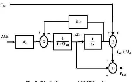
In LFC operation, the dc voltage Ed across the superconducting inductor is continuously controlled depending on the sensed area control error (ACE) signal. Moreover, the inductor current deviation is used as a negative feedback signal in the SMES control loop. So, the current variable of SMES unit is intended to be settling to its steady state value. If the load is used as a negative feedback signal in the SMES control demand changes suddenly, the feedback provides the prompt restoration of current. The inductor current must be restored to its nominal value quickly after a system disturbance, so that it can respond to the next load disturbance immediately. As a result, the energy stored at any instant is given by

𝑊𝑠𝑚= 𝑊𝑠𝑚 0+ 𝑃_𝑡𝑡₀ 𝑠𝑚 𝜏 𝑑𝜏 (13)

Where,

𝑊𝑠𝑚 0=1₂𝐿𝐼𝑑𝑜2 ,initial energy in the inductor. (14)

Equations of inductor voltage deviation and current deviation

for each area in Laplace domain are as follows ∆𝐸𝑑𝑖 𝑠 =

)

(

1

)

(

1

sT

I

s

K

s

U

sT

K

di dci id smesi

dci



















SMES

(15)

𝛥𝐼𝑑𝑖 𝑠 = _𝑠𝐿𝑖1 × ∆𝐸𝑑𝑖 𝑠 (16)

Where,

∆𝐸𝑑𝑖 𝑠 = converter voltage deviation applied to inductor in

SMES unit

KSMES = Gain of the control loop SMES Tdci = converter time constant in SMES unit Kid = gain for feedback ∆Id in SMES unit. 𝛥𝐼𝑑𝑖 𝑠 = inductor current deviation in SMES unit

The deviation in the inductor real power of SMES unit is expressed in time domain as follows

∆𝑃𝑆𝑀𝐸𝑆𝑖 = ∆𝐸𝑑𝑖𝐼𝑑𝑖+ ∆𝐸𝑑𝑖𝑖𝑑𝑖 (17)

Fig 5: Block diagram of SMES unit

In a two-area interconnected thermal power system under study with the sudden small disturbances which continuously disturb the normal operation of power system. As a result the requirement of frequency controls of areas beyond the governor capabilities SMES is located in area1 absorbs and supply required power to compensate the load fluctuations in area1. The inductor is initially charged to its rated current Ido by applying a small positive voltage. Once the current reaches the rated value it is maintained constant by reducing the voltage across the inductor to zero since the coil is superconducting [10]. Tie-line power flow monitoring is also required in order to avoid the blackout of the power system. The Input of the integral controller of each area is

𝐴𝐶𝐸𝑖= 𝛽𝑖∆𝑓𝑖+ ∆𝑃𝑡𝑖𝑒 (18) Where,

βi = frequency bias in area i ∆fi = frequency deviation in area i

∆Ptie I = Net tie power flow deviation in area SMES unit has the advantages that the time delay during

charge and discharge is quite short, Capable of controlling both active and reactive power simultaneously, loss of power is less, highly reliable and efficient also.

2.5 GAS TURBINE UNIT

Amid growing concerns about green house emissions, gas turbines have been touted as a viable option, due to their higher efficiency and the lower green house emissions compared to other energy sources and fast starting capability which enables them to be often used as peaking units that respond to peak demands. Many models representing the gas turbines have been developed over the years. A GAST model as shown in figure 6 which is one of the most commonly used dynamic models has been used in this methodology [11, 12].Gas Turbines have the advantages like Quick start-up/shut-down, low weight and size, cost of installation is less, low capital cost, Black-start capability, high efficiency requires less cranking power, pollutant emission control etc., This gives approximately two-thirds of the total power of a typical combined cycle power plant. When the load is suddenly increased the speed drops quickly but the regulator reacts and increases the fuel flow to a maximum of 100%, thereby improving the efficiency of the system.

Fig 6: Gas Turbine Model

3. Controller design using Artificial Bee

Colony Optimization technique for the

LFC assessment problem

The Artificial Bee Colony [ABC] algorithm which was introduced in 2005 by Karaboga, is used as an optimization search, simulates the intelligent foraging behavior of a honey bee swarm. It incorporates a flexible and well-balanced mechanism to adapt to the global and local exploration and exploitation abilities within a short computation time. Due to its simplicity and easy implementation, the ABC algorithm has captured much attention and has been applied to solve many practical optimization problems [13]. This method is efficient in handling large and complex search spaces and it has also been found to be robust in solving problems featuring non-linearity, no differentiability and high dimensionality. Compared with the usual algorithms, the major advantage of ABC algorithm lays in that it conducts both global search and local search in each iteration and as a result the probability of finding the optimal parameters is significantly increased, which efficiently avoid local optimum to a large extent.

In the ABC algorithm, the colony of artificial bees contains three groups of bees: Employed bees, Onlookers and Scouts. A bee waiting on the dance area for making decision to choose a food source is called an Onlooker and a bee going to the food source visited by it previously is named an employed bee. A bee carrying out random search is called a Scout.

Communication among bees about the quality of food sources is being achieved in the dancing area by performing waggle dance. In the ABC algorithm, first half of the colony consists of employed artificial bees and the second half constitutes the Onlookers. In other words, the number of employed bees is equal to the number of food sources around the hive. The employed bee whose food source is exhausted by the employed and onlooker bees becomes a scout. The main steps of the algorithm are given below [14]:

1. The search process starts with the random initialization of the bee population.

2. According to the numerical objective functions being examined, the non-dominated solution sets are stored in the archive. The archive is used to store the best estimates of the Pareto front and is updated in each search iteration. The archive updating process contains two steps:

a. Firstly, the newly generated solution sets are combined with the non-dominated solution sets already stored in the

archives. Then the dominated solutions are removed

utilized to remove the least “promising” non-dominated solutions.

3. The diversity - based performance metric, given by  [0, 1], of the solutions stored in the archive is calculated. α Estimates the level of uniformity in the distribution of solutions in the archive set, i.e., if α=1 then the solutions are uniformly distributed, whereas with α = 0.6 we may approximate that 40% of the solutions are not evenly distributed. Note that with α=0, the archive set is empty. 4. The current stage of food forage is determined according to the diversity of the archive set. Three stages or phases are distinguished: exploration, transition and exploitation.

Table 1. Bee colony structure based on diversity 

Bee type Size

Elite (i -  - s) k

Follower  k

Scout S k;

(s = 1/number of variables)

5. The bee colony structure (i.e., ratios of elite, follower and scout bees) is adjusted according to α. This adjustment aims at maximizing α (i.e., increase the distribution uniformity of the solutions). The goal is to make the solutions in the archive set evenly distributed. Note that the archive size (K) is equal to the population size.

Table 1 lists the different bee type ratios which were devised according to the following considerations:

a. In typical experiments, the generated solution sets exhibit low diversity during the initial phase (i.e., α is low). In such cases the percentage of elite bees performing the waggle dance should be high (i.e., 1-α to be high) so that exploration is emphasized. As the search proceeds, the archive set eventually becomes more diversified; the elite bee ratio should then be decreased to facilitate local fine tuning.

b. So according to the fitness (i.e., crowding distance) of individual solutions, (1-α-s)K of the bees are selected as elite ones. After that, waggle dance is performed by the elite bees. Note that the number of scout bees is fixed throughout the search.

6. The flying patterns (i.e., the bees‟ search paths) are also subjected to variation. The scout bees use a polynomial mutation operator (promoting an increase in spread) to explore the search space further. The associated mutation probability is fixed. In contrast, elite and follower bees utilize the Simulated Binary Crossover (SBX) method to exploit the near-optimal generated solutions. The adjustment of flying patterns is achieved through the automated tuning of SBX‟s distribution index. This is being performed in each iteration. The diversity-based performance metric is again utilized to drive this adjustment.

7. Then, based on the adjusted flying patterns, the bees carry out food foraging.

3.1 ABC algorithm for Decentralized

controller for LFC Problem

The following ABC algorithm [15] is adopted for the proposed study

1. Initialize the food source position Xi (solutions population) where i=1, 2 ….D

[Xi=1, 2, 3…D] (19) 2. Calculate the nectar amount of the population by means of their fitness values using:

fi *ti=1/(1+obj.fun.i J) (20) Where obj. fun.irepresents equation at solution i

3. Produce neighbor solution Vij for the Employed bees by using equation

Vij = xij + ij ( xij - xkj ) (21) Where k = (1,2,3….D) and j =( 1,2,3...N) are randomly

chosen indexes Ψ ij is a random number between [-1,1] and evaluate them as indicated in step 2.

4. Apply the greedy selection process for the Employed bees. 5. If all Onlooker bees are distributed, Go to step 9.otherwise,

Go to the next step.

6. Calculate the probability values Pi for the solution Xiusing by equation



* (22)

7. Produce the neighbor solution Vi for the Onlookers bee from the solution Xi selected depending on Pi and evaluate them.

8. Apply the greedy selection process for the Onlooker bees. 9. In ABC algorithm, providing that a position cannot be

improved further through a predetermined number of cycles, then that food source is assumed to be abandoned. The value of pre determined number of cycles is an important control parameter of the ABC algorithm, which is called “limit” for abandonment. Assume that the abandoned source is Xi and J= (1, 2, 3,…, N), then the Scout discovers a new food source to be replaced with Xi. Determine the abandoned solution for the Scout bees, if it exists, and replace it with a completely new solution Xij using the equation

Xij = Xjmin + rand (0, 1)*(Xjmax – Xjmin) (23) and evaluate them as indicated in step2.

10. Memorize the best solution attained so for.

11. If cycle=Maximum Cycle Number (MCN). Stop and print result, otherwise follow step 3.

4. RESTORATION INDICES

The availability of units in each area with their storage units, with enough margins to pick up the overload ensures whether the load disturbances or disturbance due to the outage of the units have to be given prime importance or not. In this section evaluation index namely Feasible Restoration Indices and Complete Restoration Indices are obtained and presented in the appendix A4 and A5. These restoration Indices indicate whether the system is in a condition to be restored which can be adjudged with various case studies.

The following steps are adopted to find the Restoration Indices:

I.PSR Index (I1), Based on Stability(settling time of ΔF1) 1)Read [A], [B], [Γ] matrices.

From[Y] =[C] [X]

2) Solve equation (1) i.e. 𝑋 = Ax+ Bu +Γd using Runge Kutta method [16] for a step load disturbance of 1% in area-1 of TATURIPS.

3) From the output response of ΔF1 for 1% step load change in area-1 obtain the settling time ζs of ΔF1.

4) PSR Index is obtained as the ratio between the settling time of ΔF1 and power system time constant. i.e. 𝜀1, this is referred as the Feasible Restoration Index (FRI).

II. PSR Index (I1), Based on peak overshoot /undershoot of Δf 5) Steps1 and 2 are repeated.

6) From the output response of ΔF1 for step load disturbances of 1% in area-1, the peak undershoot of ΔF1 is obtained from which PSR Index 𝜀2 is obtained.

III.PSR Index(I2),Based on the control input deviation 7) Steps 1 and 2 are repeated

8) From the control input deviationfor 1% step load change in area-1,the PSR Index 𝜀3 is obtained using Lagrangian‟s

Interpolation method [16],

PSR Index I1 ,I2 are indices of Feasible Restoration Index when the system is operating in a

normal condition with both units in operation where, I1 = Min {∈1, ∈2} and Max {∈1, ∈2}; I2 = ∈3.

The FRI computations which are based on the settling time of the output responses related to frequency deviations of both areas in TATURIPS,FRI can be given as

𝐹𝑅𝐼𝑚𝑎𝑥 = 𝑀𝑎𝑥{𝐹𝑅𝐼1, 𝐹𝑅𝐼2, 𝐹𝑅𝐼3, 𝐹𝑅𝐼4,𝐹𝑅𝐼5, 𝐹𝑅𝐼6};

𝐹𝑅𝐼𝑚𝑖𝑛 = 𝑀𝑖𝑛{𝐹𝑅𝐼1, 𝐹𝑅𝐼2, 𝐹𝑅𝐼3, 𝐹𝑅𝐼4,𝐹𝑅𝐼5, 𝐹𝑅𝐼6}; (24)

IV.Complete Restoration Indices (Based on outage) 10) Read [A], [B], [Γ] matrices.

From[Y] =[C] [X]

11) Obtain the modified [A], [B], [Γ] matrices by considering outage of one unit in area-1 of a TATURIPS.

12) Steps (3) to (8) are repeated for finding PSR Indices I1 ,I2 by considering outages in one of the units in each area of TATURIPS which are the indices for Complete Restoration Index (i.e)

𝐶𝑅𝐼 = {𝐹𝑅𝐼1, 𝐹𝑅𝐼2, 𝐹𝑅𝐼3, … , 𝐹𝑅𝐼11, 𝐹𝑅𝐼12} (25)

𝐶𝑅𝐼𝑚𝑎𝑥 = 𝑀𝑎𝑥 𝐹𝑅𝐼1, 𝐹𝑅𝐼2, 𝐹𝑅𝐼3, … , 𝐹𝑅𝐼11, 𝐹𝑅𝐼12 and

𝐶𝑅𝐼𝑚𝑖𝑛 = 𝑀𝑖𝑛{𝐹𝑅𝐼1, 𝐹𝑅𝐼2, 𝐹𝑅𝐼3, … , 𝐹𝑅𝐼11, 𝐹𝑅𝐼12} (26)

V. For Comprehensive Assessment using Indices

The above steps are repeated in carrying out the PSR Indices

(i) for a step load disturbance of 1% in area-2.

(ii) for a step load disturbance of 4% in area-1 and then in area-2.

(iii) by considering SMES unit in Area-1 and GT in Area-2 of TATURIPS (I) to (IV) and then Step (V)- (i), (ii) are repeated.

The amount of max peak (or percentage) overshoot/undershoot directly indicate the relative stability of the system. In the transient response specification the max overshoot and the rise time conflict with each other. In other words, both the max overshoot and rise time cannot be made smaller simultaneously. If one of them is made smaller and the other necessarily becomes larger [17].

6. SIMULATION RESULTS AND

OBSERVATION

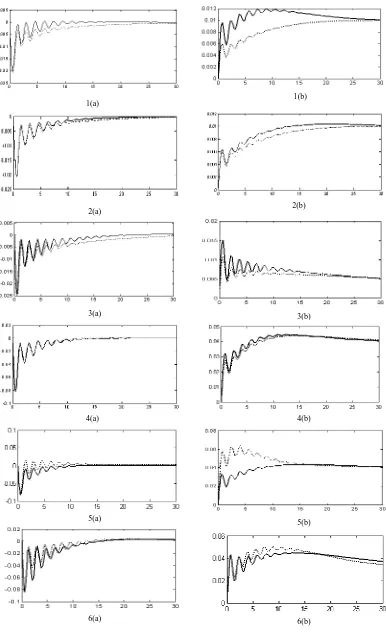
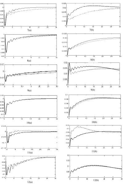
The response of the proposed controllers for the TATURIPS with SMES and GT units for different case studies of the output response of the system shows a good improvement in the performance of the system. The case study has been carried out for load change of 1% and 4% as well as with outaged conditions which can be considered as an uncertainty that occurs in an interconnected power system. The Feasible Restoration Index (FRI) are obtained for different load conditions and Complete Restoration Index (CRI) with outage of one unit and/or outage of Distribution Generation Capacity. Figures 1(a), 1(b) to 6(a), 6(b) represent the respective frequency responses and control input deviations of the case study 1 to 6 i.e. Feasible Restoration responses. Figures 7(a), 7(b) to 12(a), 12(b) represent the Complete Restoration responses. The results of the ABC tuned gain values co-ordinated with DAC, their respective settling time, FRI, CRI and also the peak over shoot value 𝜖1 of all the case study has been presented in the table 2 and 3. The proposed methodology with respect to the settling time as well as frequency deviations has been analyzed and is presented as an index for normal operation with load changes and for outage condition also.

Power System Restoration Assessment:- a) based on Settling Time

(i) If FRI or CRI is greater than 1 then more amount of distributed generation requirement is needed. b) based on peak undershoot of ΔF1 𝜖1

(i) If FRI or CRI in greater than 0.085 then the system is vulnerable and the system becomes If FRI or CRI is 0.02 ≤ 𝜖1 ≥ 0.104 then more unstable and may

result to blackout.

(ii) amount of distribution generation requirement is needed.

(iii) If FRI or CRI is greater than 0.104 not only more amount of distributed generation is required but also load shedding is preferable.

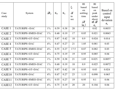
Table 2. Restoration Index Values

Case study

System ΔPd KP KI

ζs

Δf in sec

RI based

on settling

time

ΔF ϵ1

RI based

on peak under shoot of ΔF

𝜖2

Based on control

input deviation

𝜖3

CASE 1 TATURIPS +DAC 1% 0.59 0.38 20 1 0.02 0.0035

CASE 2 TATURIPS+SMES+DAC 1% 0.40 0.19 17 0.85 0.021 0.0043

CASE 3 TATURIPS+GT+DAC 1% 0.87 0.42 18 0.9 0.024 0.014

CASE 4 TATURIPS+DAC 4% 0.47 0.27 21 1.05 0.081 0.03

CASE 5 TATURIPS+SMES+DAC 4% 0.55 0.27 17.5 0.87 0.082 0.03

CASE 6 TATURIPS+GT+DAC 4% 0.75 0.19 19 0.95 0.085 0.04

CASE 7 TATURIPS+DAC 1% 0.59 0.38 21 1.05 0.025. 0.0057

CASE 8 TATURIPS+SMES+DAC 1% 0.40 0.19 18 0.9 0.025 0.0072

CASE 9 TATURIPS+GT+DAC 1% 0.87 0.42 19 0.95 0.03 0.024

CASE10 TATURIPS+DAC 4% 0.47 0.27 23 1.15 0.098 0.065

CASE11 TATURIPS+SMES+DAC 4% 0.55 0.27 19 0.95 0.1 0.04

CASE12 TATURIPS+GT+DAC 4% 0.75 0.19 20 20 0.104 0.04

 CASE 1-6: Both Units in operation

 CASE 7-12: With one unit outaged

Table 3. FRI and CRI Based on Magnitude of ΔF1 and ΔPC

SYSTEM

∈2 (ΔF)

Based on undershoot

∈3 𝛥𝑃𝑐

Based on control input deviation

FRI CRI FRI CRI

1% 4% 1% 4% 1% 4% 1% 4%

TATURIPS 0.02 0.081 0.025 0.098 0.0035 0.03 0.0057 0.065

TATURIPS + SMES+DAC

0.021 0.082 0.025 0.1 0.0043 0.03 0.0072 0.04

TATURIPS + GT+DAC

Fig 5: 1(a), 1(b) to 6(a), 6(b) Frequency deviation and Control input deviation for FRI case study; 1(a) to 6(b): x axis - Time in Seconds.

1(a), 2(a), 3(a), 4(a), 5(a), 6(a): y axis - Frequency deviations in HZ. 1(b), 2(b), 3(b), 4(b), 5(b), 6(b): y axis – Control input deviations in p.u MW.

TATURIPS (dotted line), TATURIPS with ABCPI + DAC (solid line).

6(b)

1(a) 1(b)

2(a) 2(b)

3(a) _3(b)

4(a) 4(b)

5(b) 5(a)

Fig 6: 7(a), 7(b) to 12(a), 12(b) Frequency deviation and Control input deviation for CRI case study; 7(a) to 12(b): x axis - Time in Seconds.

7(a), 8(a), 9(a), 10(a), 11(a), 12(a): y axis - Frequency deviations in HZ. 7(b), 8(b), 9(b), 10(b), 11(b), 12(b): y axis – Control input deviations in p.u MW.

TATURIPS (dotted line), TATURIPS with ABCPI + DAC (solid line).

12(a)

7(a) 7(b)

8(b) 8(a)

9(b) 9(a)

10(a)

11(a)

10(b)

11(b)

7. CONCLUSIONS

The proposed methodology has been implemented on TATURIPS considering DAC in both areas and without/with SMES and GT units in Area-1 and Area-2 respectively to meet out even under peak load conditions along with an intelligent controller in each area and to restore the system within a short span of time during inter-area oscillations thereby damping out the peak overshoots and frequency deviations due to a considerable limit of load changes and also during a outage condition. A better stability margin is obtained with both the SMES and GT units compared to that of TATURIPS without DAC, SMES and GT units. Applying the proposed methodology to the system operation, enhances the operating efficiency, securing a full restoration capability, thereby reducing the addition of new power facilities to meet out the load changes. It is clear that the restoration capability can be maintained at high level, thereby increasing the effectiveness of the electric power supply.

8. ACKNOWLEDGEMENT

The authors wish to thank the authorities of Annamalai University, Annamalainagar, TamilNadu, India for the facilities provided to prepare this paper.

9. REFERENCES

[1] Ibraheem, P. Kumar, D.P. Kothari, “Recent philosophies of automatic generation control strategies in power systems” IEEE Transactions on Power System, Vol.20, No.1, 2005, pp. 346-357.

[2] R.Roy, P.Bhatt, S.P.Ghoshal, “Evolutionary computation based Three-Area Automatic Generation Control”, Expert Systems with Applications, Vol 37, 2010, pp.5913– 24.

[3] H. Shayeghi, H.A. Shayanfar, A. Jalili, “Load Frequency Control Strategies: A state-of the-art survey for the researcher”, Energy Conversion and Management, Vol.50, No.2, 2009, pp.344-353.

[4] Chidambaram, I.A, S.Velusami, “Design of Decentralized Biased Controllers for Load Frequency Control of Interconnected Power Systems” Electric Power Components and Systems, Vol. 33, No.12, 2005, pp. 1313-1331.

[5] Elgerd,O l and Fosha,E E “ The Megawatt-FrequencyControl Problem: A new approach via optimal control theory” IEEE Trans.Pqwer Apparatus & System,Vol PAS.89,Vol 4, 1970, pp 5.

[6] Johnson,C.D “Theory of Disturbance Accommodation Controllers” in control and dynamic systems; Advances in Theory & Applications, Vol 12, Academic Press, 1976, pp.387-347.

[7] Demiroren A., “Application of a self-tuning to power system with SMES”, European Transactions on Electrical Power (ETEP), Vol. 12, N0.2, 2002, pp. 101-109.

[8] S.C.Tripathy, R.Balasubramanian, P.S.Chandramohana Nair, “Adaptive Automatic Generation Control with Super Conducting Magnetic Energy Storage in Power System”, IEEE Transactions On Energy Conversion, Vol.7, No.3, 1992, pp. 134-141.

[9] A.Demiroren, E.Yesil, “Automatic generation control With Fuzzy logic controllers in the power system including SMES units”, Electrical Power and Energy Systems, Vol:26, 2004, pp.291–305.

[10] R.J. Abraham, D. Das and A. Patra, “Automatic Generation Control of an Interconnected Hydrothermal Power System Considering Superconducting Magnetic

Energy Storage”, Electrical Power and Energy Systems; Vol 29, 2007, pp. 271-579.

[11] Soon Kiat Yee, Jovica V.Milanovic, F.Michael Hughes, “Overview and comparative Analysis of Gas Turbine Models for System Stability Studies”, IEEE Trans. On Power Systems Vol.23, No.1, 2008, pp. 108-118. [12] S.Barsali,D.poli,A.Pratico, R.Salvati, M.Sforna,R.

Zaottini, “Restoration Islands Supplied by Gas Turbine”, Electric Power System Research,Vol.78, 2008, pp. 2004-2010.

[13] D.Karaboga and B.Akay, “A Comparative Study of Artificial Bee Colony Algorithm”, Applied Mathematics

and Computation, Vol. 214, 2009, pp. 108-132. [14] S.N.Omkar, J.Senthil Nath, R.Khandelwal, G.N.Naik and S.Gopalakrishnan, “Artificial Bee Colony (ABC) forMulti-Objective Design Optimization of Composite Structures”, Applied Soft Computing, Vol. 11, Issue 1, 2011, pp. 489-499.

[15] D.Karaboga, B.Basturk, “Artificial Bee Colony (ABC) Optimization Algorithm for Solving Constrained Optimization Problems”, Advances in Soft Computing: Foundations of Fuzzy Logic and Soft Computing, LNAI.4529, springer-verlag, 2007, pp.789-798. [16] M. Shanthakumar, 1999.Computer Based Numerical Analysis, Khanna Publishers, New Delhi.

[17] Katsuhiko Ogata, 1986.Modern control Engineering, Prentice Hall of India, New Delhi.

APPENDIX

A-1 Data for the two-area interconnected thermal power system with reheat turbines (TATURIPS) [4]

Pr1=Pr2=2000MW Kp1=Kp2=120Hz/p.u Tp1=Tp2=20sec. Tt1=Tt2=0.3 sec. Tg1=Tg2=0.08sec. Kr1=Kr2=0.5 Tr1=Tr2=10 sec. R1=R2=2.4Hz/p.u MW. a12=-1

T12=0.545 p.u MW/Hz β 1 = β2 =0.425 p.u. MW/Hz

A-2 Data for the SMES unit [8] L=2H

Tdc=0.026sec Ido=4.5KA Kid=0.2 KV/KA KSMES=100KV/unit MW Idmin =4.05 KA

Idmax =6.21KA

A-3 Data for GT unit [11] T1 =10sec

T2 =0.1sec T3 =3sec Kt=1 Kr =0.04 Dturb =0.03

Max and Min Valve Position =1 and -0.1

A-4 Feasible Restoration Indices

been carried out for framing the Feasible Restoration Indices were obtained based on the settling time of the output

response of the frequency deviations in both areas as follows:

Case 1: In the TATURIPS with 1% step load disturbance in area-1; the settling time (τs1) of the frequency deviation in area-1 is obtained and FRI1 is found as

𝐹𝑅𝐼1= 𝜏𝑠1 𝑇𝑝 (24)

Case 2: In the TATURIPS considering SMES and GT in Area-1 and Area-2 respectively with 1% step load disturbance in area1 and the settling time (τs2) of the frequency deviation in area-1 is obtained and FRI2 is found as

𝐹𝑅𝐼2= 𝜏𝑠2 𝑇𝑝 (25)

Case 3: In the TATURIPS considering SMES and GT in Area-1 and Area-2 respectively with 1% step load disturbance in area2 and the settling time (τs3) of the frequency deviation in area-2 is obtained and FRI3 is found as

𝐹𝑅𝐼3= 𝜏𝑠3 𝑇𝑝 (26)

Case 4:In the TATURIPS with 4% step load disturbance in area-1; the settling time (τs4) of the frequency deviation in area-1 is obtained FRI4 is found as

𝐹𝑅𝐼4= 𝜏𝑠4 𝑇𝑝 (27)

Case 5: In the TATURIPS considering SMES and GT in Area-1 and Area-2 respectively with 4% step load disturbance in area1 and the settling time (τs5) of the frequency deviation in area-1 is obtained and FRI5 is found as

𝐹𝑅𝐼5= 𝜏𝑠5 𝑇𝑝 (28)

Case 6: In the TATURIPS considering SMES and GT in Area-1 and Area-2 respectively with 4% step load disturbance in area-2 and the settling time (τs6) of the frequency deviation in area-2 is obtained and FRI6 is found as

𝐹𝑅𝐼6= 𝜏𝑠6 𝑇𝑝 (29)

Where τs1, τs2, τs3 ,τs4, τs5,τs6 are the settling time of the (frequency deviation) output response of the system for various case studies respectively and Tp is the power system time constant. The maximum and minimum Feasible Restoration Indices are obtained as follows:

𝐹𝑅𝐼𝑚𝑎𝑥 = 𝑀𝑎𝑥{𝐹𝑅𝐼1, 𝐹𝑅𝐼2, 𝐹𝑅𝐼3, 𝐹𝑅𝐼4,𝐹𝑅𝐼5, 𝐹𝑅𝐼6} (30)

𝐹𝑅𝐼𝑚𝑖𝑛 = 𝑀𝑖𝑛{𝐹𝑅𝐼1, 𝐹𝑅𝐼2, 𝐹𝑅𝐼3, 𝐹𝑅𝐼4,𝐹𝑅𝐼5, 𝐹𝑅𝐼6 (31)

A-5 Complete Restoration Indices

Apart from the normal operating condition of the TATURIPS few other case studies like outage of one distributed generation in TATURIPS are considered with 1% and 4% step load disturbances. The various case studies obtained based on their optimal gains and their performance index is designated by CRI as follows:

Case7: In the TATURIPS with one unit outaged in area-1and with 1% stepload disturbance; the settling time is (τs7) of the frequency deviation in area-1 is obtained and FRI7 is found as

𝐹𝑅𝐼7= 𝜏𝑠7 𝑇𝑝 (32)

Case8: In the TATURIPS considering SMES and GT in Area-1 and Area-2 respectively with Area-1% stepload disturbance in area1 and the settling time (τs8) of the frequency deviation in area-1 is obtained and FRI8 is found as

𝐹𝑅𝐼8= 𝜏𝑠8 𝑇𝑝 (33)

Case9: In the TATURIPS considering SMES and GT in Area-1 and Area-2 respectively with Area-1% stepload disturbance in area2 and the settling time (τs9) of the frequency deviation in area-2 is obtained and FRI9 is obtained as

𝐹𝑅𝐼9= 𝜏𝑠9 𝑇𝑝 (34)

Case10: In the TATURIPS with one unit outaged in area-1and with 4% stepload disturbance; the settling time is (τs10) of the frequency deviation in area-1 is obtained and FRI10 is found as

𝐹𝑅𝐼10= 𝜏𝑠10 𝑇𝑝 (35)

Case11: In the TATURIPS considering SMES and GT in Area-1 and Area-2 respectively with 4% stepload disturbance in area1 and the settling time (τs11) of the frequency deviation in area-1 is obtained and FRI11 is found as

𝐹𝑅𝐼11= 𝜏𝑠11 𝑇𝑝 (36)

Case12: In the TATURIPS considering SMES and GT in Area-1 and Area-2 respectively with 4% stepload disturbance in area-2 and the settling time (τs12) of the frequency deviation in area-2 is obtained and FRI12 is obtained as

𝐹𝑅𝐼12= 𝜏𝑠12 𝑇𝑝 (37)

𝐶𝑅𝐼 = {𝐹𝑅𝐼1, 𝐹𝑅𝐼2, 𝐹𝑅𝐼3, … , 𝐹𝑅𝐼11, 𝐹𝑅𝐼12} (38)

𝐶𝑅𝐼𝑚𝑎𝑥 = 𝑀𝑎𝑥 𝐹𝑅𝐼1, 𝐹𝑅𝐼2, 𝐹𝑅𝐼3, … , 𝐹𝑅𝐼11, 𝐹𝑅𝐼12 and (39)

𝐶𝑅𝐼𝑚𝑖𝑛 = 𝑀𝑖𝑛{𝐹𝑅𝐼1, 𝐹𝑅𝐼2, 𝐹𝑅𝐼3, … , 𝐹𝑅𝐼11, 𝐹𝑅𝐼12} (40)

Apart from the FRI and CRI computations which are based on the settling time of the output response of ΔF1 in TATURIPS with various case studies, the magnitude of ΔF1 can also be used for finding FRI and CRI.

10. AUTHORS PROFILE

Dr.I.A.Chidambaram (1966) received Bachelor of Engineering in Electrical and Electronics Engineering (1987) Master of Engineering in Power System Engineering (1992) and Ph.D. in Electrical Engineering (2007) from Annamalai University, Annamalainagar. During 1988 - 1993 he was working as Lecturer in the Department of Electrical Engineering, Annamalai University and from 2007 he is