On the Estimationof the Software Effort and Schedule using Constructive Cost Model – II and Functional Point Analysis

On the Estimationof the Software Effort and Schedule

using Constructive Cost Model – II and Functional Point

Analysis

R. Chandrasekaran

Associate Professor Department of Statistics Madras Christian College Tambaram, INDIA – 600 059

R.Venkatesh Kumar

Research Scholar Department of Statistics Madras Christian College Tambaram, INDIA – 600 059

ABSTRACT

Cost estimation is an important aspect for making high-quality management decisions in the software industry. It is also related to determining how much effort and schedule are needed to complete the task on time. The challenge is to predict the accuracy of software development effort and schedule. Several models and approaches are available in the literature for such problems. This paper provides a list of software cost estimation techniquesusing Constructive Cost Model – II (COCOMO-II), function points analysis,and comparison studyto validate these models using MRE (Magnitude of Relative Error). We collected and used data from real time projects and also completed projects from one of the major information technology company for the present study.

Keywords

Software Cost Estimation methods, Functional Point Analysis, COCOMO - II, Effort Multipliers, Scale factors, and Relative Error.

1.

INTRODUCTION

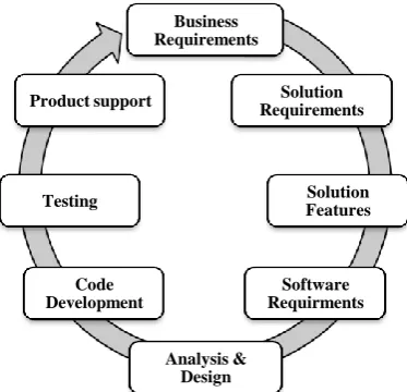
[image:1.595.329.516.540.720.2]

The software development industry is more complex andseasoned today. Asoftware industry, in general, islooking for new tools and approaches of software development methods for implementation in order to increase their profits and reduce the cost to company. It requires appropriate planning and execution to meet the goals. The challengehere is to predicate the accuracy of software development effort and schedule. The Software product is usually developed based on the market demands. Marketing and Salespeople approach their client and know theirrequirements. Senior Business Analyst creates architecture for the products along with functional and technical design specification document based on the Client’s requirement. The responsibility of project managers is to createsthe software development plan and effort/schedule estimation. Project Planning is an important phase in software development cycle; poor project forecastleads to project failures and detrimental outcomes for the project.After the initial development phase, software testing begins, and many times it is done in parallel with the development process. Documentation is also part of the development process because a product cannot be brought to the market without manuals. Once development and testing are done, the software is released and the project support cycle begins. This phase may include bug fixes and new releases. The Software Development Life Cycle shown in Figure 1.

Software cost estimation techniques can be classified into two types namely, algorithmic and non-algorithmic models. Algorithmic models are based on the statistical analysis of historical data (Hodgkinson and Garratt, 1999, Strike et al., 2001).Some of the famous algorithmicmodels are Albrecht’s Function Point (Boehm, et al., 2000;Boehm, 1995) and Putnam’s (1978), Software Life Cycle Management (SLIM) (Schofield, 1998) and Constructive Cost Model (COCOMO) (Boehm, 1981).

Non-algorithmic techniques are based on new approaches like, Parkinson (Boehm, 1981), ExpertJudgment, Price-to-Win and machine learning methodologiessuch as regression trees, rule induction, fuzzy systems, genetic algorithms, Bayesian networks, artificial neural networks, and evolutionary computation(Schofield, 1998).

This paper is structured as follows: Section II explains the literature review about the software cost estimation methods. Section III includes a detailed explanation about Cost Estimation Methods. Section IV real time software development data is used in the COCOMO – II and Functional Point Analysis models, andfinally, Section V presents conclusion of the present research.

Figure 1: Software Development Life Cycle

Business Requirements

Solution Requirements

Solution Features

Software Requirments

Analysis & Design Code

2. LITERATURE REVIEW

Software development has become an important part for many organizations; software estimation is gaining an ever-increasing importance in effective software project management. In practice, software estimation includes effort/schedule estimation, quality estimation, risk analysis, etc. Accurate software estimation can provide powerful assistance for software management decisions (Boehm, 2000). There are many methods for software cost estimation, which are divided into two groups: Algorithmic and Non-algorithmic. Usage of the both types of algorithms results inmore or less accurate cost estimation. If the requirements are known better, their performance will be better. Some popular estimation methods are discussed in detail by Khatibi and Jawawi (2011).

Boehm was the first researcherwho considered the software estimation from an economic point of view, and came up with a cost estimation model, COCOMO – 81 in 1981, after investigating a large set of data in the 1970’s (Boehm,Abts,, and Chulani,2000). Putnam also developed an early model known as SLIM, the Software Lifecycle Management, (Putnam,1978). COCOMO, SLIM and Albrect’s function point methods that measures the amount of functionality in a system, were all based on linear regression techniques by collecting data from historical project as the major input to their models. Several algorithmic methods are deliberated as the most popular methods and many researchers used the selected algorithmic methods (Musilek, et al. 2002; Yahya, et al. 2008; Lavazza and Garavaglia 2009; Yinhuan et al. 2009; Sikka et al. 2010).

Software estimation techniques can support the planning and tracking of software development projects. Efficiently controlling the expensive investment of software development is of prime importance (Gray, MacDonell and Gray, 1997; Jingzhou and Guenther, 2008; Kastro and Bener, 2008; Strike et al., 2001). Newer computational techniques are used for cost estimation that are non-algorithmic in the 1990’s. Researchers have turned their attention to a set of approaches that are based on soft computing methods. These methods include artificial neural networks, fuzzy logic models and genetic algorithms. Artificial neural network is able to generalize from trained data set. Over a known set of training data, a neural-network learning algorithm constructs rules that fit the data and predicts previously unseen data in a reasonable manner (Schofield, 1998).

ImanAttarzadeh and Siew Hock Ow (2010) proposed models based on COCOMO II and fuzzy logic to the NASA dataset and found that the proposed model performed better than ordinary COCOMO II model and also achieved results that were closer to the actual effort. The relative error for proposed model using two-side Gaussian membership functions is found to be lower than that of the error obtained using ordinary COCOMO II. A novel neuro-fuzzy Constructive Cost Model is used for software cost estimation and this model carried some of the desirable features of a neuro-fuzzy approach, such as learning ability and good interpretability, while maintaining the merits of the COCOMO model (Xishi Huang et al., 2005).

3. COST ESTIMATION METHODS

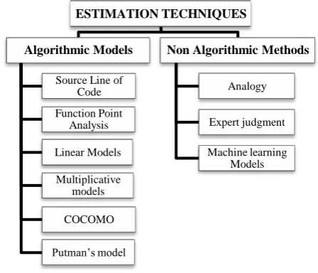
There are several methods for estimating the effort and schedule of software development project. The methods are categorised into two types which are Algorithmic and Non-algorithmic. (Khatibi andJawawi, 2011). Some of the popular estimation methods are shown in Figure 2. In the present

[image:2.595.317.541.117.309.2]

paper, we discuss the most famous and commonly used models which are COCOMO II and Function Point Analysis (FPA).

Figure 2: Estimation Techniques

3.1 COCOMO II Model

COCOMO II is one of the recentversion of COCOMO-81 model developed by Boehm in 1981. It is a non-linear regression estimation model. This model allows estimating the software cost, effort and schedule when planning a new task,and the basic elements of the model are depicted in Figure 3. It is consists of two models which are Early Design Model (EDM) and Post-Architecture Model (PAM). These models use some equations and parameters, which have been derived from previous research and practicesin software projects for estimation.

Early Design Model – EDM is used in the initial phases of software development project, while only the software architecture is being designed;the detailed information about the actual software and its overall development process are not yet to be known.

[image:2.595.316.539.580.623.2]

Post-Architecture Model – It is used in the phase when the requirement architecture is doneby the Business Analyst and the software product is ready for its development phase. (Boehm, 2000).

Figure 3: COCOMO-II Model

COCOMO-II model has many special features. The usage of this method is extremely wide and mostly results in accurate estimates. The cost drivers for COCOMO-II are rated on a 17 Effort Multipliers as shown in Table 1, and 5 scale factors as given in Table 2. Some other rating levels are also defined for scale factors including very low, low, nominal, high, very high and extra high. Usually, a quantitative value is assigned to each rating level as its weight and then the data is analysed.

ESTIMATION TECHNIQUES

Algorithmic Models

Source Line of Code

Function Point Analysis

Linear Models

Multiplicative models

COCOMO

Putman’s model

Non Algorithmic Methods

Analogy

Expert judgment

Machine learning Models

Effort

Schedule

3.1.1 Effort Multipliers

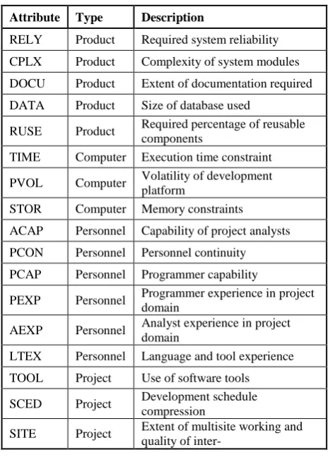
[image:3.595.52.286.176.500.2]

Cost drivers influence effort in carrying out a certain Software development project.They are some kind of characteristics associated with software development. Cost drivers are selected based on the basis that they have a linear affect on effort. There are 17 effort multipliers shown in Table 1 that are utilized by many authors who used the COCOMO II model to regulate the development effort.

Table 1. Effort Multipliers

Attribute Type Description

RELY Product Required system reliability CPLX Product Complexity of system modules DOCU Product Extent of documentation required DATA Product Size of database used

RUSE Product Required percentage of reusable components

TIME Computer Execution time constraint PVOL Computer Volatility of development

platform

STOR Computer Memory constraints

ACAP Personnel Capability of project analysts PCON Personnel Personnel continuity PCAP Personnel Programmer capability

PEXP Personnel Programmer experience in project domain

AEXP Personnel Analyst experience in project domain

LTEX Personnel Language and tool experience TOOL Project Use of software tools SCED Project Development schedule

compression

SITE Project Extent of multisite working and quality of inter-

3.1.2 Scale Factors

The application size is in the form of exponent which is an aggregate of five scale factors shown in Table 2 that describe relative economies or diseconomies of scale and arise during software projects of dissimilar magnitude.

Table 2. Scale factors

Scale Factor Reflects :

Precedentedness (PREC)

The previous experience of the organization

Development Flexibility (FLEX)

The degree of flexibility in the development process. Risk Resolution

(RESL) The extent of risk analysis carried out. Team Cohesion

(TEAM)

How well the development team knows each other and work together. Process maturity

(PMAT)

The process maturity of the organization.

3.1.3 COCOMO II - Effort and Schedule

Estimation Equations

Effort Estimation:

Person Month (PM) = A × (Size)E × 17i=1EMiEQ. 1

where E = B + 0.01 × 5j=1SFj

EMi is the Effort Multiplier(i) and SFj is the Scale Factor (j).

Baseline Effort Constantsare: A = 2.94; B = 0.91 Schedule Estimation:

Time to Develop (TDEV)= C × (PM)F _{EQ. 2}

wherePM is the Person Month F = D + 0.2 × 0.01 × 5j=1SFj

Baseline Schedule Constantsare : C = 3.67; D = 0.28

3.2 Function Point Analysis

Function Point Analysis (FPA) was developed by Allan Albrecht in 1983. The International Function Point User Group(IFPUG)is engaged in additional evolvement of FPA since 1986. The method leaves out the problems related to determination of predictable code amount. It is to be noted that function points are normalized metrics of software development project, which compute an application field and does not reflect on a technical field. At the same time, it measures application functions and data, and it won’t evaluate the source lines of code (Vickers, 2003).

3.2.1 Functions Count and Unadjusted Function

Points

Once the software requirements are formally specified then it will be challenge to count the functions. Albrecht has provided fives categories of functions to count this process: Internal Logical Files, External Interface Files, External Inputs, External Outputs and External Queries that are defined by many authors as follows:

Internal Logical Files (IFL): Any potentially unrestricted data sequence generated, used or maintained by an application can be considered as a logical file.

External Interface Files (EIF): Similar to IFL, but the given logical file is shared by some programs which includes large group of user data or leading information used in an application. This information has maintained by a different application.

External Inputs (EI): These input statements concern only user input orders, which are related to changes in the internal data structure. They do not concern user input orders, which are aimed only at control of program implementation. External Outputs (EO): The calculation scheme is similar to that ones related to the input orders. All unique user data or control data leaving the external frontier of the measured system count as output orders.

[image:3.595.53.286.583.728.2]

Functions are identified for given categories, and then functions complexity are also rated as low, average, or high as shown in Table 3.

Table 3. Function Count Weighting Factors

Factors Low Average High

Internal Logical Files _ x 7 _ x 10 _ x 15 External Interface Files _ x 5 _ x 7 _ x 10 External Inputs _ x 3 _ x 4 _ x 6 External Outputs _ x 4 _ x 5 _ x 7 External Queries _ x 3 _ x 4 _ x 6 Each function count is multiplied by the weight depending on its complexity and all of the function counts are added to get the count for the entire system called unadjusted function points (UFP). This calculation is summarized by the following equation:

UFP = 3i=1 5j=1WijXijEQ. 3

whereWij is the weight for row i, column j, and Xij is the function count in cell (i, j) of the Table 3 (Kemerer, 1993).

3.2.2 Adjusted Function Points

UFP explains a good notion of the number functions in a system, but it does not take into account the environment variables for determining effort required to program the system. For example, a software system with very high performance is required, then additional effort is needed to make sure that the software is written as competently as possible. Albrecht recognized this when developing the FP model and created a list of fourteen “general system characteristics that are rated on a scale from 0 to 5 in terms of their likely effect for the system being counted.” (Kemerer, 1993). The characteristics considered by Kemerer are given in Table 4.

Table 4. Factor of Technical Complexity

F1 Data

communications F8 On-line update F2 Distributed data

processing F9 Reusability F3 Performance F10 Complex

processing F4 Heavily used

configuration F11 Installation ease F5 Transaction rate F12 Operational ease F6 On-line data entry F13 Multiple sites F7 End-user efficiency F14 Facilitate change The ratings given to each of the characteristics mentioned above Fi’s are then entered into the formula in Equation 4 to get the Value Adjustment Factor (VAF):

VAF = (TDI × 0.01) + 0.65 EQ. 4 TDI= 14i=1DIiEQ. 5

where TDI is a factor of technical complexity, and DIi,its resulting degree of influence. It concerns a calibrating parameter of effort and indicates an influence of all the 14 factors. Each of them is rated by a six-point scale (0 - 5) according to a relevant degree of influence (TDI) on application.

Finally, the Adjusted Function Point (AFP) is obtained as the product of UFP and VAF (AFP) count:

AFP = UFP ×VAF EQ. 6

Effort estimation of the coding size and total cost of the project can be obtained from adjusted function points. To begin with, it is necessary to specify the effort and a price of one function point. Based on this, the total costs necessary for the project development can be calculated. Depending on the programming language in which the software project is developed, the size of the source code, which corresponds to one function point, is assessed. The estimation of code size for given programming language (Kemerer,1993 and IFPUG,2010).

The effort of new project is estimated as a share of number of points for new project divided by number of points per months:

E = _FP′FP

M EQ. 7

where FP

′

/M is an average amount of function points declining on one person-month and it is determined from the finished projects. An estimation of project development duration in months can be calculated by relation

3.3 Validation of COCOMO II and FPA

In this section, we try to show the minimum distance between estimated effort and actual effort of the development project. The estimation effort performance is accomplished by computing several metrics including Magnitude of Relative Error (MRE). This is a popular parameter which is used for performance evaluation of methods

MRE = (Actual Effort – Predicted Effort )

Actual Effort EQ.8

4. METHODOLOGY

Our main objective of this section is to estimate the effort/schedule of existing project and compare it with actual effort/schedule using COCOMO II Post-Architecture Model and Function Point Analysis. For the present experiment, we have used a real time development project, which was developed in SAS (Statistical Analysis System) from one of the major Information Technology.

The software was developed in SAS language with experienced team of analysts and developers. This data is collected from one of the major Information TechnologyCompany.Actual code extent is 23.80 Kilo (thousand) Line of Code (KLOC), Actual effort for this project is 30.12 person-month and actual time is 9.4 months.

4.1 COCOMO II – Effort/Schedule

Estimation

COCOMO II Post-Architecture Modelis the most popular

method used for software cost estimation. In this section, we used a real-time project to estimate the project effort based on COCOMO II metrics. Table 5

shows the cost drivers and their adjusted amounts and

[image:5.595.75.522.125.500.2]

Develop(TDEV) and Magnitude of Relative Error (MRE)are estimated.

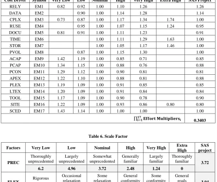
Table 5. Effort Multiplier

Cost Driver Symbol Very Low Low Nominal High Very High Extra High SAS Project

RELY EM1 0.82 0.92 1.00 1.10 1.26 1.26

DATA EM2 0.90 1.00 1.14 1.28 1.14

CPLX EM3 0.73 0.87 1.00 1.17 1.34 1.74 1.00

RUSE EM4 0.95 1.00 1.07 1.15 1.24 0.95

DOCU EM5 0.81 0.91 1.00 1.11 1.23 0.91

TIME EM6 1.00 1.11 1.29 1.63 1.00

STOR EM7 1.00 1.05 1.17 1.46 1.00

PVOL EM8 0.87 1.00 1.15 1.30 1.00

ACAP EM9 1.42 1.19 1.00 0.85 0.71 0.85

PCAP EM10 1.34 1.15 1.00 0.88 0.76 0.88

PCON EM11 1.29 1.12 1.00 0.90 0.81 0.81

APEX EM12 1.22 1.10 1.00 0.88 0.81 0.88

PLEX EM13 1.19 1.09 1.00 0.91 0.85 0.85

LTEX EM14 1.20 1.09 1.00 0.91 0.84 0.84

TOOL EM15 1.17 1.09 1.00 0.90 0.78 0.90

SITE EM16 1.22 1.09 1.00 0.93 0.86 0.80 0.80

SCED EM17 1.43 1.14 1.00 1.00 1.00 1.00

𝐄𝐟𝐟𝐨𝐫𝐭 𝐌𝐮𝐥𝐭𝐢𝐩𝐥𝐢𝐞𝐫𝐬𝐢 𝟏𝟕

[image:5.595.79.521.419.659.2]

𝐢=𝟏 _0.3403

Table 6. Scale Factor

Factors Very Low Low Nominal High Very High Extra

High

SAS project

PREC

Thoroughly unprecedented

Largely unprecedented

Somewhat unprecedented

Generally familiar

Largely familiar

Thoroughly

familiar _3.72

6.2 4.96 3.72 2.48 1.24 0

FLEX Rigorous

Occasional relaxation

Some relaxation

General conformity

Some conformity

General

goals _3.04

5.07 4.05 3.04 2.03 1.01 0

RESL Little (20%) Some (40%) Often (60%)

Generally (75%)

Mostly (90%)

Full

(100%) _4.24

7.07 5.65 4.24 2.83 1.41 0

TEAM

Very difficult interactions

Some difficult interactions

Basically cooperative interactions

Largely cooperative

Highly cooperative

Seamless

interactions _3.29

5.48 4.38 3.29 2.19 1.1 0

PMAT

SW-CMM Level 1 Lower

SW-CMM Level 1 Upper

SW-CMM Level 2

SW-CMM Level 3

SW-CMM Level 4

SW-CMM

Level 5 _4.68

7.8 6.24 4.68 3.12 1.56 0

Effort Estimation = 2.94 *23.801.0997 * 0.3403 = 32.66 [PM] Schedule Estimation = 3.67 * 32.660.31794 = 11.11815 [M] MRE = (30.12 – 32.66)

30.12

=

0.084

It is to be noted from the above estimates, that the difference between the actual and estimated project efforts, Schedule time and the MRE are very small. Thisis only a sample project

4.2 FPA – Effort/Schedule Estimation

[image:6.595.74.255.330.592.2]

Albrecht(1983) has presented the Function Point Analysis to measure the functionality of the software project. Following this method, estimates of indicators are obtained and shown in Table 7.

Table 7. Estimation of Unadjusted Function Points

Weigh Simple Average Complex Total Internal

Logical Files,

2 x 7 3 x 10 8 x 15 164 External

Interface Files,

1 x 5 2 x 7 7 x 10 89 External

Inputs, 3 x 3 4 x 4 12 x 6 97 External

Outputs 1 x 4 1 x 5 5 x 7 44 External

Queries 2 x 3 2 x 4 5 x 6 44

UFP 438

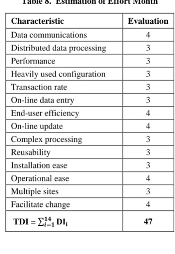
Table 8. Estimation of Effort Month

Characteristic Evaluation

Data communications 4 Distributed data processing 3

Performance 3

Heavily used configuration 3

Transaction rate 3

On-line data entry 3

End-user efficiency 4

On-line update 4

Complex processing 3

Reusability 3

Installation ease 3

Operational ease 4

Multiple sites 3

Facilitate change 4

TDI = 𝟏𝟒𝒊=𝟏𝐃𝐈𝐢 47

Effort Estimation = 490.56

14.30 = 34.30 [PM] Schedule Estimation = 490.560.4 = 11.92 [M]

MRE = (30.12 – 34.30)

30.12

=

0.138

The difference between the actual project effort and estimated project effort is small and MRE is 0.138 whenusing Functional Point Analysis.

5. CONCLUSION

Software estimation is an important process for making high-quality management decisions in the software industry. It is

to be noted that the most important reason for the software project failure is inaccurate estimation of parameters in early stages of the project planning.So, the methods of estimation play an essential part in achievingthe accurate and reliable estimates. In the present study, many of the available estimation techniques have been illustrated systematically to arrive at the estimation of parameters of interest.Software estimation includes cost estimation, effort/schedule estimation, quality estimation, risk analysis, etc. Accurate estimates can provide powerful support when software management decisions are made, for instance, accurate cost estimation can help an organization to better investigate the feasibility of a project and to effectively manage the software project in the development life cycle. Performance of each estimation method depends on several parameters such as difficulty of the project,schedule of the project, expertise of the staff, development method, etc. From the data obtained from a real-time software project associated with an IT industry, certain metrics and their estimateshave been obtained using COCOMO – II and Function Point Analysis. We are working towards the improvement of the accuracy and precision of the estimates of various indices associated with software projects to help the decision makers to give more reliable software cost and schedule estimates.

6. REFERENCES

[1] Albrecht, A.J. and Gaffney, J.E., 1983, Software function, source lines code, and development effort prediction: a software science validation, IEEE Transaction of Software Engineering, Vol.9, No.6, pp.639-648.

[2] Boehm B. W., 1981, Software Engineering Economics, Englewood Cliffs, Prentice-Hall, New Jersey.

[3] Boehm, B.W., 1995, Cost models for future software lifecycle processes: COCOMO 2.0, Ann. SoftwareEng. Vol.1, pp.45-60.

[4] Boehm, B. W., 2000,Software Cost Estimation with COCOMO II, Prentice Hall, New Jersey.

[5] Boehm B. W., Abts, C., and Chulani, S., 2000, Software development cost estimation approaches-A survey, Ann. Software Eng., Vol.10, pp.177-205.

[6] Futrell, R.T., Shafer D.F., and Shafer, L.I., 2002, Quality Software Project Management, Pearson Education Pvt. Ltd., Delhi.

[7] Hodgkinson, A.C. and P.W. Garratt, 1999, Aneurofuzzy cost estimator, Proc. of the 3rdInternational Conference on Software Engineering and Applications, (SEA’99), pp: 401-406.

[8] IFPUG, 1994,The International Function Point Users Group, Function Point Counting Practices Manual, Release 4.0, Westerville, Ohio.

[9] Iman A., and Siew Hock Ow, 2010, A Novel Algorithmic Cost Estimation Model Based on Soft Computing Technique, Journal of Computer Science, Vol.6, No. 2, pp. 117-125.

[10] Jones. C., 2007,Estimating software costs: Bringing realism to estimating, 2nd ed. New York: McGraw-Hill. [11] Kemerer, C.F., 1993, Reliability of Function Points

[12] Kemerer, C.F., 1987, An Empirical Validation of Software Cost Estimation Models, Communications of the ACM, Vol. 30, No.5, pp. 416-429.

[13] Khatibi, V. and Jawawi, D.N.A., 2011, Software Cost Estimation Methods: A Review, Journal of Emerging Trends in Computing and Information Science, Vol.2, No.1, pp.21-29.

[14] Lavazza, L. and Garavaglia. C., 2009, Using function points to measure and estimate real-time and embedded software: Experiences and guidelines,Proc. of the 3rd International Symposium on Empirical Software Engineering and Measurement,pp.100-110.

[15] Musilek, P., Pedrycz, W., Nan Sun and Succi, G.,2002, On the sensitivity of COCOMO II software cost estimation model, Proc. of the Eighth IEEE Symposium on Software Metrics, pp.13-20.

[16] Putnam, L.H., 1978. A general empirical solution to themacro software sizing and estimating problem.IEEE Trans. Software Eng., No.4, pp. 345-361.

[17] Schofield C., 1998, Non-Algorithmic effort estimation techniques. Technical Reports,TR98-01, Department of Computing, Bournemouth University, England.

[18]Strike, K., K. El-Emam and N. Madhavji, 2001,Software cost estimation with incomplete Data,IEEE Trans. Software Eng., Vol.27, pp.890-908.

[19] Sikka, G., Kaur, A., and Uddin, M. 2010, Estimating function points: Using machine learning and regression models,Proc. of the 2nd International

ConferenceEducation Technology and Computer (ICETC), Vol.3, pp.52-56.

[20] Vickers, P., 2010, An Introduction to Function Point Analysis, Manual of the Function Point User Group, New Jersey, ISBN 978-0-9753783-4-2.

[21] Xishi Huang, Danny Ho, Jing Ren, Luiz F. Capretz, 2005, Improving the COCOMO model using a neuro-fuzzy approach, Journal Applied Soft Computing, Vol. 7, pp. 29-40.

[22] Yahya, M.A., Ahmad, R., and Sai Peck Lee, 2008, Effects of Software Process Maturity on COCOMO II’s Effort Estimation from CMMI Perspective, Proc. of the IEEE International Conferenceon Research, Innovation and Vision for the Future, RIVF. pp.255-262.

[23] Yinhuan, Z., Beizhan, W., Yilong Z., andLiang, S., 2009, Estimation of software projects effort based on function point, Proc. of the 4th International Conference onComputer Science & Education, ICCSE,pp. 941-943. [24] Function :http://en.wikipedia.org/wiki/Function_point [25] Software_testing:

http://en.wikipedia.org/wiki/Software_testing [26] qatfaq1.html

http://www.softwareqatest.com/qatfaq1.html

[27] atfaq2.html http://www.softwareqatest.com/qatfaq2.html [28] http://decgradschool.bournemouth.ac.uk/ESERG/