The Principle and Accuracy Analysis of Automatic Target Scoring System Based on Acoustic Detection

2019 2nd International Conference on Informatics, Control and Automation (ICA 2019) ISBN: 978-1-60595-637-4

The Principle and Accuracy Analysis of Automatic Target-Scoring

System Based on Acoustic Detection

Xue-hai TANG

, Ju-hua YIN

, Hai-guang LI

and Xing-hao FENG

Mailbox 790-1, Korla, P.R. China 2

Bayinguoleng Vocational and Technical College, Korla, P.R. China *Corresponding author

Keywords: Automatic Target-Scoring System, Acoustic Detection, TDOA, Location Accuracy.

Abstract. This paper derived the principles of 3-station TDOA (time difference of arrival) location and 4-station TDOA location based on acoustic detection, and the theoretical accuracy analysis of the two kinds of TDOA location is carried out. Under the assumption that the time difference measurement error is linearly related to the distance of sound propagation, the influence of different station distribution modes on the location accuracy is analyzed. The results show that with reasonable distribution of measurement points, the automatic target-scoring system based on acoustic detection can meet the requirement of impact measurement in missile test range. Compared with traditional target-scoring system, the automatic target-scoring system based on acoustic detection has its unique advantages, such as unattended, fast, automatic and high-accuracy. The research has engineering reference and practical applied value.

Introduction

The attack accuracy has always been an important index for evaluating missile test. In missile test tasks, it is usually required that the range report the real-time measurement results of the landing point of missile. At present, many optical measuring equipments are deployed around the theoretical landing point, after the missile landed, the observation angle data is sent to the remote control station in real time to calculate the coordinates of the landing point. This measurement method consumes lots of time, labour and material resources. Therefore, it is necessary to research a new method of measuring the landing point to make up for the shortcomings of the existing methods. Multipoint passive TDOA location technology has been widely used in military, civil and other industries. Multipoint location technology has developed from basic three-station TDOA to multi-station and multi-station networking technology [1, 2]. The landing or airburst of missile will produce a huge sound, so the multi-station TDOA location based on acoustic detection can be considered for measuring the landing or airburst point.

The TDOA location requires three or more detection stations. The principles of TDOA location with three stations and four stations are deduced in this paper. The location accuracy is related to the location of the detection stations and the target. In this paper, the accuracies of 3-station TDOA and 4-station location are theoretically analyzed, and the location accuracies of several typical station distribution ways are simulated and analyzed. Finally, the ideal station distribution way is obtained, which has practical value.

Principle of Multi-station TDOA Location Based on Acoustic Detection

Principle of 2D 3-station TDOA Location

O (0,0)

A(x1,y1)

B(x2,y2) P(x,y)

r1

r2

r0

x y

Figure 1. Diagram of 2D 3-station TDOA Location.

As shown in Fig. 1, assume that P is the point to be measured. O, A and B are three acoustic detection points. P, O, A and B are all on the same plane, which corresponds to the landing situation of the missile. Without loss of generality, it is advisable to set O as the origin of coordinates. Assume that the distances from P to the three detection points arer₀, r₁and r₂, respectively. The time difference

between the sound reaches points A and O is t₁, which for points B and O is t₂ , the sound velocity isv. According to the geometric relation, the following formulas can be obtained:

2

2 2 2 2

1 1 1 0 1 1

2 2 2 2 2 2 2 0 2 ( ) ( ) ( ) ( )

r v t r r x x y y x y

r v t r r x x y y x y

           

 

          

 . (1)

Transform Eq. 1, we can get

2 2 2

1 1 1 1 1 1 0

2 2

2 2 2 2 2 0

2 2 1 ( ) 2 1 ( ) 2

x x y y x y r r r

x x y y x y r r r

 _{         }

 

          



. (2)

Let matrixes 1 1 2 2 x y x y       

A , (3)





x y



X , (4)

2

2 2 2

2 2 2

1 1 1 1 0

1 1 0

2 2 0

2 2 2 0 1 ( ) 2 1 ( ) 2

x y r r r

k r r

k r r

x y r r r

 _{     }    _{    }   _{  }     _{     }       

B , (5)

then Eq. 2 can be expressed as



AX B. (6) When points O, A and B are not collinear, the matrix A is invertible, thusX A B1 . Let

11 12 1 21 22 a a a a        

then

11 1 12 2 11 1 12 2 0 11 12 0

21 1 22 2 21 1 22 2 0 21 22 0

( )

( )

x a k a k a r a r r b b r

y a k a k a r a r r b b r

          



           

 . (8)

Bring Eq. 8 into the formula 2 2 0

r  x y , we can obtain

2 2 2 2 2 2

12 22 0 11 12 21 22 0 11 21 0 0

0=(b b  1) r 2(b b b b ) r (b b ) a r   b r c. (9)

By solving the above quadratic equation, the value of r0can be obtained, and r0 0. For quadratic

Eq.9, when b24ac0, there is no solution, it is due to the acoustic detection errors. When

2

4 0

b  ac , there are two solutions, if the two solutions are both negative, this is obviously impossible and which is also due to the acoustic detection errors. If one of the two solutions is positive and the other is negative, then bring the positive one in Eq. 8 and the coordinates of the target point P can be obtained. If the two solutions are both positive, then a fuzzy solution appears, the correct solution can be obtained by adding an acoustic detection station or adding the azimuth detection function of the acoustic detection station.

Principle of 3D 4-station TDOA Location

O _(0,0,0) C (x3,x3,y3)

B(x2,y2,z2)

P (x,y,z)

r3

r1

r0

x

z

A(x1,y1,z1)

y

r2

Figure 2. Diagram of 3D 4-station TDOA Location.

As shown in Fig. 2, assume that P is the point to be measured. O, A, B and C are four acoustic detection points. P, O, A, B and C are distributed in 3D (three-dimensional) space, which corresponds to the airburst situation of the missile. Similar to the above, set O as the origin of coordinates. Assume that the distances from P to the four detection points arer₀,r₁,r₂andr₃, respectively. The time

difference between the sound reaches points A and O is t₁, which for points B and O is t₂, which

for points C and O is t₃, the sound velocity isv. Similar to the above deductions, Let matrixes

1 1 1

2 2 2

3 3 3

x y z

x y z

x y z

 

 

  

 

 

A , (10)





x y z



2 2 2 2

1 1 1 1 1 0

1 1 0

2 2 2 2

2 0

2 0

3 0

2 2 2 2

3 0

2

2 2 2 2

3

3 3 2 3

1 ( ) 2 1 ( ) 2 1 ( ) 2

x y z r r r

k r r

k r r

x y z r r r

k r r

x y z r r r

 _{      }               _{  } _        _{  }       _{  }  _{      }     

B , (12)

we can obtain



AX B. (13) When O, A, B and C are not coplanar, the matrix A is invertible, thusX A B1 . Let

11 12 13 1

21 22 23

31 32 33

a a a

a a a

a a a

           

A , (14)

then

11 1 12 2 13 3 11 1 12 2 13 3 0 11 12 0

21 1 22 2 23 3 21 1 22 2 23 3 0 21 22 0

31 1 32 2 33 3 31 1 32 2 33 3 0 31 32 0

( )

( )

( )

x a k a k a k a r a r a r r b b r

y a k a k a k a r a r a r r b b r

z a k a k a k a r a r a r r b b r

                                                 

. (15)

Bring Eq. 15 into the formula r₀  x2y2z2 , we can get

2 2 2 2 2 2 2

12 22 32 0 11 12 21 22 31 32 0 11 21 31

2

0 0

0=(b b b 1) r 2(b b b b +b b ) r (b b b )

a r b r c

         

     . (16)

Similarly, by solving the above quadratic equation, the value of r0can be obtained, then the

coordinates of point P are obtained. In the same way, the ambiguity can be eliminated by adding an acoustic detection station or adding the azimuth detection function of the acoustic detection station.

Accuracy Analysis of Multi-station TDOA Location

Accuracy Analysis of 2D 3-station TDOA Location

By using differential method on Eq. 1, the following formulas can be obtained:

2

1 1

1

1 0 1 0

2 2

2 0 2 0

( ) ( ) ( )

( ) ( ) ( )

x x x y y y

v d t dx dy

r r r r

x x x y y y

v d t dx dy

r r r r

           _{ }        

. (17)

Let





T

dT  d t d t , (18)





1 1

1 0

2

1 0

2

2 0 2 0

( ) ( )

( ) ( )

x x x y y y

r r r r

x x x y y y

r r r r

 

 _{ } 

 

 



 

 _{ } 

 

 

C , (20)

then Eq. 17 can be expressed as

d v d

  

C X T. (21) Thus

dX  v CdT. (22) Where Cis the generalized inverse of C. It can be seen from Eq. 22 that the location error

(dx dy, ) is correlated with the sound velocity v, the time difference measurement error dT , the locations of the acoustic detection stations and the positions of point P relative to the acoustic detection stations. The location accuracy is

2 2

dx dy

   . (23)

Accuracy Analysis of 3D 4-station TDOA Location

Similar to the above deduction, let





T

dT  d t d t d t , (24)





dX  dx dy dz , (25)

2

1 1 1

1 0 1 0 1 0

2 2

2 0 2 0 2 0

3 3

3 0 3

3

0 3 0

( ) ( ) ( )

( ) ( ) ( )

( ) ( ) ( )

x x x y y y z z z

r r r r r r

x x x y y y z z z

r r r r r r

x x x y y y z z z

r r r r r r

  _  _  _ 

 

 

 _{  } 

_    _

 

 _{  } 

  

 

 

C , (26)

the following formula can be obtained:

dX  v CdT. (27) Where Cis the generalized inverse of C. It can be seen from Eq. 27 that the location error

(dx dy dz, , ) is correlated with the sound velocity v, the time difference measurement error dT , the locations of the acoustic detection stations and the positions of point P relative to the acoustic detection stations. The location accuracy is

2 2 2

dx dy dz

    . (28)

Simulation Analysis of Station Distribution

Simulation Analysis of 3-station TDOA Location

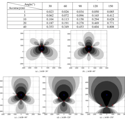
the distance of sound propagation, d( t_i)=(r_ir₀) 340 0.001 , that is to say, the average error of sound propagation per second is 1 millisecond. Fig. 3 shows the distribution areas of location accuracy when the angle AOB is 30°, 60°, 90°, 120° and 150°. The deeper the color, the higher the location accuracy. The specific statistical results are shown in Table 1. The numerical value represents the proportion of the area where the corresponding accuracy is located to the total area. The total area is the square area with a side length of 6000 meters as shown in the figure. As can be seen from the figure and the table, when the angle AOB is 150°, the area of high- accuracy (less than 10 meters) is relatively large.

Table 1. Simulation Results of 3-station Location Accuracy.

Angle(°)

Accuracy(m) 30 60 90 120 150

1 0.023 0.026 0.034 0.050 0.085 5 0.062 0.072 0.096 0.165 0.412 10 0.104 0.113 0.158 0.294 0.628 20 0.187 0.191 0.278 0.469 0.771 40 0.353 0.349 0.453 0.604 0.808

(a) ∠AOB=30° (b) ∠AOB=60°

(c) ∠AOB=90° (d) ∠AOB=120° (e) ∠AOB=150°

Figure 3. Simulation Analysis Chart of 3-station Location Accuracy.

Simulation Analysis of 4-station TDOA Location

Four-station TDOA location can realize 3D spatial location, which is corresponding to the case of missile airburst. According to the actual situation, it is easy to build a tower less than 20 meters high near the landing point of the missile, and one of the acoustic detection stations can be placed on the top of the tower. Therefore, let the coordinates of point C be (0, -20, 20) and OA=OB=1000m, similarly, the location accuracy is simulated by changing the angle between OA and OB. Assuming that the measurement error of TDOA is linearly related to the distance of sound propagation,

0

( _i)=( _i ) 340 0.001

values represent the proportion of the volume of the region where the corresponding accuracy is located to the total volume. The total volume is the volume of the cube with a side length of 6000 meters as shown in the figure. As can be seen from the figure and the table, when the angle AOB is 120°, the region of high- accuracy (less than 10 meters) is relatively large.

Table 2. Simulation Results of 4-station Location Accuracy.

Angle (°)

Accuracy (m) 30 60 90 120 150

1 0.013 0.019 0.019 0.000 0.000 5 0.086 0.131 0.243 0.312 0.066 10 0.174 0.232 0.348 0.533 0.348 20 0.309 0.368 0.474 0.651 0.846 40 0.489 0.530 0.619 0.755 0.941

(a) ∠AOB=30° (b) ∠AOB=60°

(c) ∠AOB=90° (d) ∠AOB=120° (e) ∠AOB=150°

Figure 4. Simulation Analysis Chart of 4-station Location Accuracy.

Conclusion

References

[1] H. Gao and Z. Li, Research on orientating precision algorithm of time-difference passive orientation system of multi-station, Systems Engineering and Electronics, 27(4) (2005), pp. 578-581.

[2] Q. Miao, D. Wu and Y. Mao, Application of multiple stations passive position technology in local position network, Modem Radar, 29(8) (2007), pp. 12-14.

[3] Q. Zhang, Accuracy-affected factors analyses of multi-station time difference positioning and measurement system on sea-borne dynamic platform, Ship Electronic Engineering, 38(12) (2018), pp.176-179.

[4] X. Dou, H. Li and B. Xu, Station arrangement strategy based on GDOP of TDOA location using external illuminators, Electronic Information Warfare Technology, 33(5) (2018), pp. 37-40.