A smoothing inexact Newton method for variational inequalities with nonlinear constraints

R E S E A R C H

Open Access

A smoothing inexact Newton method for

variational inequalities with nonlinear

constraints

Zhili Ge

_{, Qin Ni}

_{and Xin Zhang}

*_{Correspondence:}

gezhilyly66@126.com

1_{College of Science, Nanjing}

University of Aeronautics and Astronautics, Nanjing, 211106, China

2_{Basic Sciences Department,}

Nanjing Polytechnic Institute, Nanjing, 210048, China Full list of author information is available at the end of the article

Abstract

In this paper, we propose a smoothing inexact Newton method for solving variational inequalities with nonlinear constraints. Based on the smoothed Fischer-Burmeister function, the variational inequality problem is reformulated as a system of

parameterized smooth equations. The corresponding linear system of each iteration is solved approximately. Under some mild conditions, we establish the global and local quadratic convergence. Some numerical results show that the method is effective.

Keywords: variational inequalities; nonlinear constraints; inexact Newton method; global convergence; local quadratic convergence

1 Introduction

We consider the variational inequality problem (VI for abbreviation), which is to find a vectorx∗∈such that

VI(,F) x–x∗Fx∗≥, ∀x∈, ()

whereis a nonempty, closed and convex subset ofRn_{andFis a continuous differentiable}

mapping fromRnintoRn. In this paper, without loss of generality, we assume that

:=x∈Rn|g(x)≥, ()

whereg:Rn_→Rm _andg

i:Rn→R, (i∈I={, , . . . ,m}) are twice continuously

differ-entiable concave functions. When=Rn

+, VI reduces to the nonlinear complementarity

problem (NCP for abbreviation)

x∗∈Rn₊, Fx∗∈Rn₊, x∗Fx∗= . () Variational inequalities have important applications in mathematical programming, economics, signal processing, transportation and structural analysis [–]. So, there are various numerical methods which have been studied by many researchers; e.g., see [].

A popular way to solve the VI(,F) is to reformulate () to a nonsmooth equation via a KKT system of variational inequalities and an NCP-function. It is well known that the

KKT system of VI(,F) can be given as follows:

⎧ ⎪ ⎪ ⎨ ⎪ ⎪ ⎩

F(x) –∇g(x)λ= , g(x) –z= ,

λ≥,z≥, λz= ,

()

and the NCP-functionφ(a,b) is defined by the following condition:

φ(a,b) =  ⇐⇒ a≥,b≥,ab= . ()

Then problem () and () is equivalent to the following nonsmoothing equation:

⎛ ⎜ ⎝

F(x) –∇g(x)λ g(x) –z

φ(λ,z)

⎞ ⎟

⎠= . ()

Hence, problem () and () can be translated into ().

We all know that the smoothing method is a fundamental approach to solve the nons-mooth equation (). Recently, there has been strong interest in snons-moothing Newton meth-ods for solving NCP [–]. The idea of this method is to construct a smooth function to approximateφ(λ,z). In the past few years, there have been many different smoothing functions which were employed to smooth equation (). Here, we define

H(μ,x,λ,z) :=

⎛ ⎜ ⎜ ⎜ ⎝

μ F(x) –∇g(x)λ

g(x) –z (μ,λ,z)

⎞ ⎟ ⎟ ⎟

⎠, ()

where

(μ,λ,z) :=

⎛ ⎜ ⎜ ⎝

ϕ(μ,λ,z)

.. . ϕ(μ,λm,zm)

⎞ ⎟ ⎟

⎠ ()

and

ϕ(μ,a,b) =a+b–a_+b_+μ_, ∀(_μ,a,b)∈_R_{. ()}

It follows from equations ()-() thatH(μ,x,λ,z) =  is equivalent toμ=  and (x,λ,z) is the solution of (). Thus, we may solve the system of smoothing equationH(μ,x,λ,z) =  and reduceμto zero gradually while iteratively solving the equation.

In reality, variational inequalities with nonlinear constraints are more attractive. These problems have wide applications in economic networks [], image restoration [, ] and so on. So, in this paper, under the framework of smoothing Newton method, we propose a new inexact Newton method for solving VI(,F) with nonlinear constraints, which ex-tends the scope of constraints. We also prove the global and local quadratic convergence and present some numerical results which show the efficiency of the proposed method.

Throughout this paper, we always assume that the solution set of problem () and (), denoted by∗, is nonempty.R+andR++ mean the nonnegative and positive real sets.

Symbol · stands for the -norm.

The rest of this paper is organized as follows. In Section , we summarize some useful properties and definitions. In Section , we describe the inexact Newton method formally and then prove its local quadratic convergence. We also give global convergence in Sec-tion . In SecSec-tion , we report our numerical results. Finally, we give some conclusions in Section .

2 Preliminaries

In this section, we denote some basic definitions and properties that will be used in the subsequent sections.

Definition . The operatorFis monotone if, for anyu,v∈Rn_,

(u–v)F(u) –F(v)≥;

Fis strongly monotone with modulusμ>  if, for anyu,v∈Rn_,

(u–v)F(u) –F(v)≥μu–v;

Fis Lipschitz continuous with a positive constantL>  if, for anyu,v∈Rn,

F(u) –F(v)≤Lu–v.

The following lemma gives some properties ofHand its corresponding Jacobian.

Lemma . Let H(μ,x,λ,z)be defined by().Assume that F is continuously differentiable and strongly monotone, g is twice continuously differentiable concave, (μ∗,x∗,λ∗,z∗) in R+×Rn×Rm×Rm is the solution of H(μ,x,λ,z) = ,the rows of∇g(x∗)are linearly

independent and(λ∗,z∗)satisfies the strict complementarity condition.Then (i) H(μ,x,λ,z)is continuously differentiable onR+×Rn×Rm×Rm.

(ii) ∇H(μ∗,x∗,λ∗,z∗)is nonsingular,where

∇H(μ,x,λ,z) =

⎛ ⎜ ⎜ ⎜ ⎝

   

 ∇F(x) –∇_{g(x)λ –∇g(x) }

 ∇g(x)  –I

Dμ  Dλ Dz

⎞ ⎟ ⎟ ⎟

⎠, ()

Dμ=vec

– μ λ_i +z_i +μ

Dλ=diag

 – λi λ_i+z

i +μ

(i= , . . . ,m),

Dz=diag

 – zi λ_i+z

i +μ

(i= , . . . ,m) and

∇_g(x)λ=m j=

∇_g

j(x)λj.

Proof It is not hard to show thatHis continuously differentiable onR++×Rn×Rm×Rm.

FromH(μ∗,x∗,λ∗,z∗) = , by () we get thatμ∗=  easily. Since (λ∗,z∗) satisfies the strict complementarity condition, i.e.,λ∗_i,z_i∗are not equal to  at the same time, we have thatH is also continuously differentiable on (μ∗,x∗,λ∗,z∗). That is, (i) holds.

Now, we prove (ii). Let q= (q,q,q,q) ∈R+×Rn×Rm ×Rm, q = (q), q=

(q,q, . . . ,qn),q= (q,q, . . . ,qm),q= (q,q, . . . ,qm), and

∇Hμ∗,x∗,λ∗,z∗

⎛ ⎜ ⎜ ⎜ ⎝ q q q q ⎞ ⎟ ⎟ ⎟ ⎠= . ()

Hence, we have

⎧ ⎪ ⎪ ⎪ ⎪ ⎪ ⎪ ⎨ ⎪ ⎪ ⎪ ⎪ ⎪ ⎪ ⎩

q= , ()

(∇F(x∗) –∇g(x∗)λ∗)q–∇g(x∗)q= , ()

∇g(x∗_)q

–q= , ()

Dλ∗q+Dz∗q= , ()

where

Dλ∗=diag

 – λ ∗ i

λ∗

i +z∗i

, Dz∗=diag

 – z ∗ i

λ∗

i +zi∗

.

We can observeq=  easily by ().

Next, we discuss formula (). The full form of () can be described as follows:

⎛ ⎜ ⎜ ⎜ ⎜ ⎜ ⎜ ⎜ ⎝

( –√ λ∗

λ∗_+z∗_)q+ ( – z∗ √

λ∗_+z∗_)q

( –√ λ∗

λ∗_+z∗_)q+ ( – z∗ √

λ∗_+z∗_)q

.. . ( –√ λ∗m

λ∗m+z∗m

)qm+ ( – z ∗ m

√

λ∗m+z∗m

)qm ⎞ ⎟ ⎟ ⎟ ⎟ ⎟ ⎟ ⎟ ⎠ = . ()

According to the strict complementarity condition of (λ∗,z∗), we haveλ∗_i ≥,z∗_i ≥, λ∗_iz∗_i =  andλ∗_i,z_i∗are not equal to  at the same time. Ifz∗_i = , thenλ∗_i > , and

 – λ ∗ i

λ∗_i+z∗_i

= ,

 – z ∗ i

λ∗_i+z∗_i

From () we get thatqi=  andqiqi= . Similarly, ifλ∗i = , thenz∗i > . We get that

qi=  andqiqi= . Hence,qq= .

Multiplying the equation of () byq on the left-hand side and usingqq= , we have

q_∇gx∗q= . ()

Multiplying the equation of () byq_ on the left-hand side and using (), we have q_∇Fx∗–∇gx∗λ∗q= . ()

Meanwhile, because F is strongly monotone, we have that ∇F(x∗) is a positive defi-nite matrix. Besides, sincegis concave andλ∗is nonnegative, we have that∇_g(x∗_)λ∗₌

m

j=∇gj(x∗)λ∗j are nonpositive definite matrices, which implies that (∇F(x∗) –

∇_g(x∗_)λ∗_{) is a positive definite matrix. So, we get thatq}

=  by ().

Substitutingq=  into () and using the rows of∇g(x∗) are linearly independent, we

getq= . Substitutingq=  into (), we getq= . Hence we haveq= , which implies

that∇H(μ∗,x∗,λ∗,z∗) is nonsingular. This completes the proof.

3 The inexact algorithm and its convergence

We are now in the position to describe our smoothing inexact Newton method formally by using the smoothed Fischer-Burmeister function () to solve the variational inequalities with nonlinear constraints. We also show that this method has local quadratic conver-gence.

Algorithm .(Inexact Newton method)

Step . Letw= (x,λ,z)and(μ,w_)∈R

++×Rn+mbe an arbitrary point.Chooseμ> 

andγ∈(, )such thatγ μ_< .

Step . IfH(μk_,wk₎_{= ,then stop.}

Step . Compute(μk,wk)by

H(μk,wk_{) +∇Hμ}k_,wk

μk

wk

=

ρkμ

rk

, ()

whereρk=ρ(μk,wk) :=γmin{,H(μk,wk)},andrk∈Rn+msuch thatrk ≤ρkμ.

Step . Setμk+=μk+μkandwk+=wk+wk.Setk:=k+ and go to Step. Remark 

() In theory, we useH(μk_,wk₎_{= as a termination of Algorithm .. In practice, we}

useH(μk,wk)≤εas a termination rule, whereεis a pre-set tolerance error. () It is obvious that we haveρk≤γH(μk,wk).

() From () and (), we haveμk+=ρkμ> for anyk≥.

Now, we are ready to analyze the convergence. The quadratic convergence of Algo-rithm . is given below.

() There exists a setD⊂R+×Rn+mwhich contains(μ∗,w∗)such that for any

(μ_,w_{)∈D,the iterate points(μ}k_,wk_{)generated by Algorithm.are well defined,}

remain inDand converge to(μ∗,w∗); ()

μk+–μ∗,wk+–w∗≤βμk–μ∗,wk–w∗, ()

whereβ:= (L+ γ μ∇H(μ∗,w∗)_)∇H(μ∗_,w∗₎–_.

Proof According to Theorem .. in [] and Lemma ., we give the proof in detail. Denote

u=

μ w

, u∗=

μ∗ w∗

, u=

μ

w

, vk=

ρkμ

rk

.

By Step  of Algorithm ., we have

vk≤ρkμ+rk≤ρkμ≤γ μH

uk. ()

According to Lemma ., we get that∇H(u∗) is nonsingular. Then there exist a positive constantt¯< _β and a neighborhoodN(u∗,t) of¯ u∗such thatL¯t≤ ∇H(u∗), and for any u∈N(u∗,t), we have that¯ ∇H(u) is nonsingular and

_∇H(u)–∇Hu∗≤∇H(u) –∇Hu∗≤Lu–u∗, ()

where the first inequality follows from the triangle inequality and the second inequality follows from the Lipschitz continuity. Hence we have

_∇H(u)≤∇Hu∗ ()

for anyu∈N(u∗,¯t). Similarly, by the perturbation relation (..) in [], we know that ∇H(u) is nonsingular and

_∇H(u)–_≤ ∇H(u∗)–

 –∇H(u∗)–(∇_{H(u) –}∇H(u∗))≤∇H

u∗–. ()

Besides, for anyt∈[, ], we have

u∗+t(u–u∗)∈N(u∗,¯t) andH(u) –H(u∗) =_∇H[u∗+t(u–u∗)](u–u∗)dt. FromH(u∗)= , we have

H(u)≤

 

_∇Hu∗+tu–u∗u–u∗dt≤∇Hu∗u–u∗. ()

According to Algorithm ., for anyuk∈N(u∗,¯t),k≥, we have

uk+–u∗

=∇Huk–∇Hukuk–u∗–Huk–Hu∗+vk =∇Huk–

×





∇Huk–∇Hu∗+tuk–u∗uk–u∗dt+vk

. ()

Taking norm of both sides, we get

uk+–u∗

≤∇Huk–





L( –t)uk–u∗dt+vk

≤∇Hu∗–

 Lu

k_–u∗

+ γ μHuk

≤∇Hu∗–

 Lu

k_–u∗_{+ γ μ}_∇Hu∗_uk_–u∗

=L+ γ μ∇Hu∗∇Hu∗–uk–u∗, ()

where the first inequality follows from the Lipschitz continuity, the second inequality fol-lows from (), and the third inequality folfol-lows from ().

According to the definition ofβ and the condition of¯t< 

β, we get thatu

k_converges

tou∗. Besides, () also holds. This completes the proof.

4 The global inexact algorithm and its convergence

Now, we start our globally convergent method by using the global technique in Algo-rithm .. We choose a merit functionh(μ,w) =_H(μ,w)_{and modify (μ}k_,wk_{) such}

that

–μk,wk∇hμk,wk≥δμk,wk∇hμk,wk. ()

We use line search to find a step-lengthtk_{∈(, ] such that}

hμk+tkμk,wk+tkwk≤hμk,wk+ρ¯tk∇hμk,wkμk,wk, ()

∇hμk+tkμk,wk+tkwkμk,wk≥ ¯σ∇hμk,wkμk,wk ()

and

μk+tkμk∈R++, wk+tkwk∈Rn+m, ()

whereρ¯∈(, .),σ¯∈(ρ¯, ),δ∈(, ).

Algorithm .(Global inexact Newton method)

Step . Choose(μ_,w_)∈R

++×Rn+mto be an arbitrary point.Chooseγ∈(, )such that

γ μ<

.Chooseρ¯∈(, .),σ¯ ∈(ρ¯, ),δ∈(, ).

Step . Find(μk_,wk_{)by solving().If()is not satisfied,then chooseτ}

kand compute

μk,wk= –∇Hμk,wk∇Hμk,wk+τkI –

∇hμk,wk, ()

such that()is satisfied.

Step . Find a step-lengthtk_{∈(, ]satisfying()-().}

μk+=μk+tk_μk_,wk+_=wk_+tk_wk_{.Setk:=k+ and go to Step.}

Remark  In Step , if () is not satisfied, then the technique in [], pp.-, is used to chooseτk. From Lemma . in [], it is not difficult to findtkthat can satisfy ()-().

In order to obtain the global convergence of Algorithm ., throughout the rest of this paper, we define the level setL(μ,w) ={(μ,w)|h(μ,w)≤h(μ,w)}for (μ,w)∈R++×

Rn+m_.

Theorem . Suppose that∇H(μ,w)is Lipschitz continuous inL(μ,w_{).Then we have}

lim

k→∞∇h

μk,wk= .

Proof The proof follows Theorem . in [] and condition ().

Theorem . Let(μ,w_)∈R

++×Rn+m,H(μ,x,λ,z)be defined by(). Assume that

∇H(μ,w)is Lipschitz continuous inL(μ_,w_),tk_{= is admissible and()is satisfied for}

all k≥k,∇H(μ∗,w∗)is nonsingular where kis sufficiently great,and(μ∗,w∗)is a

lim-ited point of{(μk_,wk_{)}generated by Algorithm..Then the sequence{(μ}k_,wk_)}converges

to(μ∗,w∗)quadratically.

Proof From Theorem ., we have

lim

k→∞∇h

μk,wk= ,

where∇h(μk_,wk_{) =∇H(μ}k_,wk_)H(μk_,wk_{). That is, the sequence{(μ}k_,wk_{)}is convergent.}

Since∇H(μ∗,w∗) is nonsingular and (μ∗,w∗) is a limited point of{(μk,wk)}generated by Algorithm ., we have

lim

k→∞H

μk,wk= .

According to the assumption that there existsksuch thattk=  is admissible and ()

is satisfied for allk≥k,{(μk,wk)}can be generated by Algorithm . fork>k. We can

get the conclusion from Theorem . directly. This completes the proof.

5 Numerical results

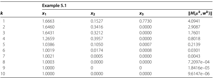
In this section, we present some numerical results for Algorithm .. All codes are written in Matlab and run on a RTM i-M personal computer. In the algorithm, we choose γ = .. We also useH(μk_,wk_{) ≤}–_{as the stopping rule for all examples.}

Table 1 Numerical results for Example 5.1 withx0= (0, 1, 1)

Example 5.1

k x1 x2 x3 H(μk, wk)

1 1.6663 0.1527 0.7730 4.0941

2 1.6460 0.3416 0.0000 2.9087

3 1.6431 0.3212 0.0000 1.7601

4 1.2659 0.3957 0.0000 0.8018

5 1.0386 0.1050 0.0007 0.2139

6 1.0019 0.0174 0.0008 0.0301

7 1.0021 0.0005 0.0000 0.0043

8 1.0003 0.0000 0.0000 7.2097e–04

9 1.0000 0 0 1.8416e–05

10 1.0000 0.0000 0.0000 9.6147e–06

Example .(see []) Let

F(x) =

⎛ ⎜ ⎝

x+ .x– .x+ .x– 

–.x+x+ .x+ .

.x– .x+ x– .

⎞ ⎟ ⎠

and

g(x) = –x_– .x_– .x_+ .

It is verified that the problem has the solutionx∗= (, , ) easily. The initial point isx₌

(, , ) andμ= ..

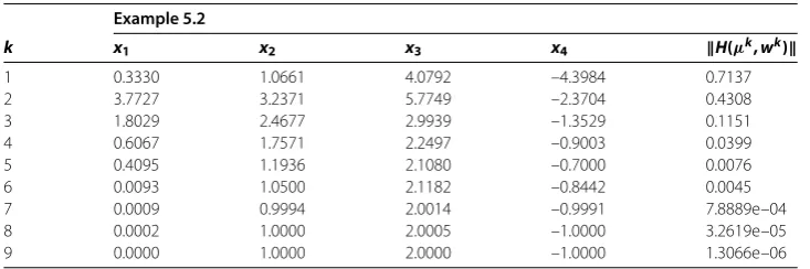
Example . This example is derived from []. Because the original problem is an opti-mization problem, we give its form of variational inequalities by the optimality condition, i.e.,

F(x) =

⎛ ⎜ ⎜ ⎜ ⎝

x– 

x– 

x– 

x+ 

⎞ ⎟ ⎟ ⎟

⎠, g(x) = ⎛ ⎜ ⎝

–x

–x–x–x–x+x–x+x+ 

–x

– x–x– x+x+x+ 

–x_–x_–x_– x+x+x+ 

⎞ ⎟ ⎠.

The solution of Example . isx∗= (, , , –). The initial point isx_{= (, , , ) and}

μ= ..

In Tables -, ‘k’ means the number of iterations, ‘H(μk,wk)’ means the -norm of H(μk_,wk_{). From Tables -, we can observe that Algorithm . can find the solution in a}

smaller number of iterations for the above two examples. In order to further show the effi-ciency of Algorithm ., we give other two examples where the dimension of the problems is from  to ,.

In the following tests, we solvewof the linear systems by using GMRES(m) package withm= , allowing a maximum of  cycles (, iterations). And we chooseμ_{as a}

random number in (, ).

Table 2 Numerical results for Example 5.2 withx0= (0, 0, 0, 0)

Example 5.2

k x1 x2 x3 x4 H(μk, wk)

1 0.3330 1.0661 4.0792 –4.3984 0.7137

2 3.7727 3.2371 5.7749 –2.3704 0.4308

3 1.8029 2.4677 2.9939 –1.3529 0.1151

4 0.6067 1.7571 2.2497 –0.9003 0.0399

5 0.4095 1.1936 2.1080 –0.7000 0.0076

6 0.0093 1.0500 2.1182 –0.8442 0.0045

7 0.0009 0.9994 2.0014 –0.9991 7.8889e–04

8 0.0002 1.0000 2.0005 –1.0000 3.2619e–05

9 0.0000 1.0000 2.0000 –1.0000 1.3066e–06

Table 3 Numerical results for Example 5.3

Example 5.3

n No.it CPU H(μk, wk₎

100 8 0.3120 7.7321e–06

200 8 0.4992 2.9356e–06

300 9 0.7956 2.5000e–06

400 9 1.1700 1.3077e–06

600 9 2.1840 1.8843e–06

800 9 3.8220 2.1879e–06

1,000 9 5.6004 2.0789e–06

we also add some nonlinear constraints to the problem. In this example,

F(x) = ⎛ ⎜ ⎜ ⎜ ⎜ ⎜ ⎜ ⎝  –· · ·    · · ·  · · ·   · · · –   · · ·  ⎞ ⎟ ⎟ ⎟ ⎟ ⎟ ⎟ ⎠ ⎛ ⎜ ⎜ ⎜ ⎜ ⎜ ⎜ ⎜ ⎝ x x x .. . xn ⎞ ⎟ ⎟ ⎟ ⎟ ⎟ ⎟ ⎟ ⎠ + ⎛ ⎜ ⎜ ⎜ ⎜ ⎜ ⎜ ⎜ ⎝ – – – .. . – ⎞ ⎟ ⎟ ⎟ ⎟ ⎟ ⎟ ⎟ ⎠

, g(x) =

⎛ ⎜ ⎜ ⎜ ⎜ ⎜ ⎜ ⎜ ⎜ ⎜ ⎜ ⎜ ⎜ ⎜ ⎝

x+ 

x+ 

· · · xn+ 

 –x 

 –x 

· · ·  –x_n

⎞ ⎟ ⎟ ⎟ ⎟ ⎟ ⎟ ⎟ ⎟ ⎟ ⎟ ⎟ ⎟ ⎟ ⎠ .

Example . The example is the NCP.F(x) =D(x) +Mx+q. The components ofD(x) are Dj(x) =dj·arctan(xj), wheredjis a random variable in (, ). The matrixM=AA+B,

whereAis ann×nmatrix whose entries are randomly generated in the interval (–, ), and the skew-symmetric matrixBis generated in the same way. The vectorqis generated from a uniform distribution in the interval (–, ).

In Tables -, ‘n’ means the dimension of problems, ‘No.it’ means the number of itera-tions, ‘CPU’ means the cpu time in seconds. ‘H(μk,wk_{)’ means the -norm ofH(μ}k_,wk_).

From Tables -, we find that Algorithm . is robust to the different sizes for these two problems. Moreover, the iterative number is insensitive to the size of problems in our al-gorithm. In other words, our algorithm is more effective for two problems.

6 Conclusions

Table 4 Numerical results for Example 5.4

Example 5.4

n No.it CPU H(μk_{, w}k₎

100 8 0.4992 3.5558e–07

200 8 1.1388 3.0105e–06

300 8 2.3244 4.7536e–06

400 8 4.5552 7.7267e–06

600 9 13.1665 8.8521e–07

800 9 25.3346 1.4537e–06

1,000 9 41.4027 2.0736e–06

some mild conditions, we establish the global and local quadratic convergence. Further-more, we also present some preliminary numerical results which show efficiency of the algorithm.

Acknowledgements

The first author is supported by Funding of Jiangsu Innovation Program for Graduate Education (KYZZ15_0087) and the Fundamental Research Funds for the Central Universities. The second author is supported by NSFC (11471159; 11571169; 61661136001) and the Natural Science Foundation of Jiangsu Province (BK20141409).

Competing interests

The authors declare that they have no competing interests.

Authors’ contributions

The authors contributed equally and significantly in writing this paper. All authors read and approved the final manuscript.

Author details

1_{College of Science, Nanjing University of Aeronautics and Astronautics, Nanjing, 211106, China.}2_{Basic Sciences}

Department, Nanjing Polytechnic Institute, Nanjing, 210048, China.3_{School of Arts and Science, Suqian College, Suqian,}

223800, China.

Publisher’s Note

Springer Nature remains neutral with regard to jurisdictional claims in published maps and institutional affiliations.

Received: 15 March 2017 Accepted: 22 June 2017

References

1. Ferris, MC, Pang, JS: Engineering and economic applications of complementarity problems. SIAM Rev.39, 669-713 (1997)

2. Fischer, A: Solution of monotone complementarity problems with locally Lipschitzian functions. Math. Program.76, 513-532 (1997)

3. Li, YY, Santosa, F: A computational algorithm for minimizing total variation in image restoration. IEEE Trans. Image Process.5, 987-995 (1996)

4. Facchinei, F, Pang, JS: Finite-Dimensional Variational Inequalities and Complementarity Problems, Volumes I and II. Springer, Berlin (2003)

5. Chen, BT, Harker, PT: Smooth approximations to nonlinear complementarity problems. SIAM J. Optim.7, 403-420 (1997)

6. Chen, BT, Xiu, NH: A global linear and local quadratic noninterior continuation method for nonlinear complementarity problems based on Mangasarian smoothing functions. SIAM J. Optim.9, 605-623 (1999) 7. Qi, LQ, Sun, DF, Zhou, GL: A new look at smoothing Newton methods for nonlinear complementarity problems and

box constrained variational inequalities. Math. Program.87, 1-35 (2000)

8. Qi, LQ, Sun, DF: Improving the convergence of non-interior point algorithms for nonlinear complementarity problems. Math. Comput.229, 283-304 (2000)

9. Tseng, P: Error Bounds and Superlinear Convergence Analysis of Some Newton-Type Methods in Optimization. Nonlinear Optimization and Related Topics. Springer, Berlin (2000)

10. Ma, CF, Chen, XH: The convergence of a one-step smoothing Newton method for P0-NCP base on a new smoothing NCP-function. Comput. Appl. Math.216, 1-13 (2008)

11. Zhang, J, Zhang, KC: A variant smoothing Newton method for P0-NCP based on a new smoothing function. J. Comput. Appl. Math.225, 1-8 (2009)

12. Rui, SP, Xu, CX: A smoothing inexact Newton method for nonlinear complementarity problems. J. Comput. Appl. Math.233, 2332-2338 (2010)

14. Rui, SP, Xu, CX: A globally and locally superlinearly convergent inexact Newton-GMRES method for large-scale variational inequality problem. Int. J. Comput. Math.3, 578-587 (2014)

15. Toyasaki, F, Daniele, P, Wakolbinger, T: A variational inequality formulation of equilibrium models for end-of-life products with nonlinear constraints. Eur. J. Oper. Res.236, 340-350 (2014)

16. Ng, MK, Weiss, P, Yuan, XM: Solving constrained total-variation image restoration and reconstruction problems via alternating direction methods. SIAM J. Sci. Comput.32, 2710-2736 (2010)

17. Dennis, JE Jr, Schnabel, RB: Numerical Methods for Unconstrained Optimization and Nonlinear Equations. Prentice Hall, Philadelphia (1983)

18. Nocedal, J, Wright, SJ: SJ: Numerical Optimization, 2nd edn. Springer, New York (1999)

19. Fukushima, M: A relaxed projection method for variational inequalities. Math. Program.35, 58-70 (1986)

20. Charalambous, C: Nonlinear least pth optimization and nonlinear programming. Math. Program.12, 195-225 (1977) 21. Ahn, BH: Iterative methods for linear complementarity problems with upperbounds on primary variables. Math.