R E S E A R C H
Open Access
A smoothing and regularization
predictor-corrector method for nonlinear
inequalities
Haitao Che
**Correspondence:
[email protected] School of Mathematics and Information Science, Weifang University, Weifang, Shandong 261061, China
Abstract
For a system of nonlinear inequalities, we approximate it by a family of parameterized smooth equations via a new smoothing function. We present a new smoothing and regularization predictor-corrector algorithm. The global and local superlinear convergence of the algorithm is established. In addition, the smoothing parameter
μ
and the regularization parameterε
in our algorithm are viewed as differentindependent variables. Preliminary numerical results show the efficiency of the algorithm.
MSC: 90C33; 90C30; 15A06
Keywords: nonlinear inequalities; predictor-corrector algorithm;P0-function; smoothing function
1 Introduction
Consider the following system of nonlinear inequalities:
f(x)≤, (.)
wheref(x) = (f(x),f(x), . . . ,fn(x))andfi:Rn→Ris a continuously differentiable function
fori= , , . . . ,n. This problem finds applications in data analysis, set separation problems, computer-aided design problems and image reconstructions [–]. Among various solu-tion methods for the inequality problems [–], the smoothing-type methods receive much attention [–] which first transform the problem as a system of nonsmooth equa-tions and approximate it by a smooth equation and then solve it by the smoothing Newton methods. Since the derivative of the underlying mapping may be seriously ill-conditioned, which may prevent the smoothing methods from converging to a solution of the prob-lem, a perturbed regularization technique is introduced to overcome this drawback [, , ]. In , Huanget al.proposed a predictor-corrector smoothing Newton method for nonlinear complementarity problem with aPfunction based on the perturbed minimum function []. The method was shown to be locally superlinear convergent under the as-sumptions that allV ∈∂H(z*) are nonsingular andf(x) is locally Lipschitz continuous aroundx*.
In this paper, motivated by the smoothed penalty function for constrained optimiza-tion [], we construct a new smoothing funcoptimiza-tion for nonlinear inequalities, and thus we
can approximate the nonsmooth system of transformed equations by a system of smooth equations. We develop a regularization smoothing predictor-corrector method for solv-ing the problem by modifysolv-ing and extendsolv-ing the method in []. Besides choossolv-ing an ar-bitrarily starting point, the presented algorithm is simpler than the predictor-corrector noninterior continuation methods developed by Burke and Xu [].
The rest of this paper is organized as follows. In Section , we review some preliminar-ies to be used in the subsequent analysis and introduce a new smoothing function and its properties. In Section , we present a smoothing and regularization predictor-corrector method for solving the nonlinear inequalities and establish the global and local conver-gence of the proposed algorithm. Preliminary numerical experiments are reported to show the efficiency of the algorithm in Section .
To end this section, we introduce some notations used in this paper. The set ofm×k matrices with real entries is denoted byRm×k,Rn
+(Rn++) denotes the nonnegative (positive) orthant inRn. The superscript denotes the transpose of a matrix or a vector. Define N={, , . . . ,n}, and for any vectora∈Rn, we letD
a denote the diagonal matrix whose
i-th diagonal element isai.udenotes the -norm of a vectoru∈Rn. For a continuously
differentiable functionf :Rn→Rm, we denote the Jacobian off atx∈Rnbyf(x). 2 Smooth reformulation of nonlinear inequalities
In this section, we first review some definitions and basic results, and then introduce a new smoothing function and show its properties.
Definition . A matrixM∈Rn×nis said to be aP
-matrix if every principle minor ofM is nonnegative.
Definition . A functionF:Rn→Rnis said to be aP
-function if for allx,y∈Rnwith x=y, there exists an indexi∈Nsuch that
xi=yi, (xi–yi)
Fi(x) –Fi(y)
≥.
For aP-matrix, the following conclusion holds [].
Lemma . If M∈Rn×nis a P-matrix,then every matrix of the form
Da+DbM
is nonsingular for all positive definite diagonal matrices Da,Db∈Rn×n.
Definition . Suppose thatG:Rn→Rmis a locally Lipschitz function.Gis said to be
semi-smooth atxifGis directionally differentiable atxand
lim
V∈∂G(x+th),h→h,t→+
Vh
exists for anyh∈Rn, where∂G(x) denotes the generalized derivative in [].
[]. Convex functions, smooth functions, piecewise linear functions, convex and concave functions, and sub-smooth functions are examples of semi-smooth functions. A function is semi-smooth at xif and only if all its component functions are. The composition of semi-smooth functions is still a semi-smooth function.
Lemma .[] Suppose thatϕ:Rn→Rmis a locally Lipschitz function semi-smooth at x.
Then
(a) for anyV∈∂ϕ(x+th),h→,
Vh–ϕ(x;h) =oh,
(b) for anyh→,
ϕ(x+h) –ϕ(x) –ϕ(x;h) =oh. For problem (.), based on the function
x+=
max{,x}, . . . ,max{,xn}
, forx∈Rn,
it can be transformed into the following system of equations []:
f(x)+= . (.)
Since problem (.) is a nonsmooth equation, the classical Newton methods cannot be used to solve it. Following the ideas in [, , ], we adopt the following smoothing function to approximate the nonsmooth equation
φ(μ,a) =
a+μ
ln +ln
+cosha
μ
, (.)
where a smoothing parameterμ> andcoshx=ex+e–x. This new smoothing function has the following properties.
Lemma . For any(μ,a)∈R++×Rn,it holds that
() φ(·,·)is continuously differentiable at any(μ,a)∈R++×Rn.
() Letφ(,a) =limμ→φ(μ,a),thenφ(,a) =a+.
() ∂φ∂(μa,a)≥at any(μ,a)∈R++×Rn.
Proof () is straightforward, so we only prove () and (). For (), following the ideas in [], we have
|a|≈ϕ(μ,a) =μ
ln +ln
+cosha
μ
.
Furthermore, one can obtain the estimate []
|a|–ϕ(μ,a)≤μ e
Thenφ(,a) =a+.
For (), by a simple calculation, we can show
∂ϕ(μ,a)
∂a =
sinha
μ
+coshμa ∈(–, ),
then∂φ(∂μa,a)≥ at any (μ,a)∈R++×Rn. We complete the proof.
Letz= (μ,ε,x)∈R++×R++×Rnand
H(z) =H(μ,ε,x) =
⎛ ⎜ ⎝
μ ε (z)
⎞ ⎟
⎠, (.)
where
(z) =(μ,εx) =
⎛ ⎜ ⎜ ⎝
φ(μ,f(x)) .. .
φ(μ,fn(x)) ⎞ ⎟ ⎟
⎠+εx. (.)
Define a merit function
ψ(z) =H(z)=μ+ε+(z). (.)
Then the inequalities (.) can be reformulated as the following nonlinear equations:
H(z) =H(μ,ε,x) = . (.)
Theorem . Let H(μ,ε,x)be defined as(.).Then
(a) H(μ,ε,x)is continuously differentiable at anyz= (μ,ε,x)∈R++×R++×Rnwith its
Jacobian
H(z) =
⎛ ⎜ ⎝
μ(z) x x(z)
⎞ ⎟
⎠, (.)
where
μ(z) =φμμ,f(x)
, . . . ,φμμ,fn(x)
,
x(z) =φxμ,f(x)+εI= diag
+ sinh
fi(x)
μ
+coshfi(x)
μ
:i∈N
f(x) +εI.
(b) Iff is aP-function,thenH(z)is nonsingular at anyR++×R++×Rn.
Theorem . in []. We also note that diag{( + sinh
fi(x)
μ
+coshfiμ(x)) :i∈N} andεIare positive
diagonal matrices, we know thatx(z) is nonsingular by Lemma ., which implies that H(z) is also nonsingular. This completes the proof.
3 Algorithm and convergence
In this section, we first describe our algorithm and then we reveal the global convergence analysis of the algorithm. Now, we are at a position to give the description of our smooth-ing predictor-corrector algorithm.
Algorithm .
Step . Take δ∈(, ), σ ∈(, ). Let e= (μ,ε, )∈R++×R++×Rn and x∈Rn is
an arbitrary point. Choose z= (μ
,ε,x) and parameter γ ∈(, ) such that
γH(z) ≤,γ μ+γ ε< . Setk= .
Step . IfH(zk)= , then stop. Otherwise, letβ
k=β(zk)whereβ(z)is defined byβ(z) = γH(z).
Step . Predictor step. IfH(zk) ≥, setzˆk:=zk and go to Step . Otherwise, compute ˆzk= (μˆ
k,εˆk,xˆk)∈R×R×Rnby
Hzk+Hzkzk=βkH
zke. (.)
If
ψzk+ˆzk≤ψzk, (.)
then setzˆk=zk+zˆk. Otherwise, setzˆk=zk.
Step . Corrector step. IfH(zk)= , then stop. Otherwise, computez˜k= (μ˜ k,ε˜k, x˜k)∈R×R×Rnby
Hzˆk+Hzˆkzk=βzˆke. (.)
Letlkbe the smallest nonnegative integerlsuch that
ψzˆk+δlz˜k≤ –σ –γ(μ+ε)
δlψˆzk. (.)
Setλk=δlkandzk+:=zˆk+λk˜zk. Step . Setk:=k+ and return to Step .
Remark . IfH(zk) ≥, then Algorithm . solves only one linear system of
To prove the convergence of Algorithm ., first, define the set
=z= (μ,ε,x)∈R++×R++×Rn|μ≥β(z)μ,ε≥β(z)ε
.
The following lemmas show that Algorithm . is well defined and generates an infinite sequence with some good features.
Lemma . If f is a continuously differentiable P-function,then Algorithm .is well
defined.In addition,μk> ,εk> and zk= (μk,εk,xk)∈for any k≥.
Proof Sincefis a continuously differentiablePfunction, then it follows from Theorem . that the matrixH(z) is nonsingular foru> ,ε> . Sinceu> ,ε> by the choice of an initial point, we may assume, without loss of generality, thatμk> ,εk> , we show that
ˆ
μk> ,εˆk> . If the predictor step is accepted, then by (.),
ˆ
μk=βkH
zkμ, (.)
ˆ
εk=βkH
zkε, (.)
otherwise, we havezk=ˆzk, which meansμ
k=μˆk,εk=εˆk. Thus, we obtainμˆk> ,εˆk> .
Furthermore,H(zk) andH(ˆzk) are nonsingular which means that (.) and (.) are well
defined.
Givenk≥, for anyα∈(, ], let
R(α) =Hzˆk+α˜zk–Hzˆk–αHzˆkz˜k. (.)
NotingH(·) is continuously differentiable, we obtainR(α)=o(α). Then, it follows from (.) and (.) that
Hzˆk+αz˜k=Hzˆk+αHzˆkz˜k+R(α)
≤( –α)Hˆzk+R(α)+αγHˆzke ≤( –α)Hˆzk+αγ(μ+ε)H
ˆ
zk+o(α)
≤ – –γ(μ+ε)
αHzˆk+o(α). (.)
Therefore, from (.), it shows that there exists a positive numberα¯ ∈(, ] such that for allα∈(,α¯] andσ∈(, ),
Hzˆk+αz˜k≤ –σ –γ(μ+ε)
αHzˆk (.)
holds, which implies
ψzˆk+αz˜k≤ –σ –γ(μ+ε)
αψzˆk.
That is, the nonnegativelksatisfying (.) can be found, which demonstrates that (.) is
Fork= , sinceβ(z) =γH(z) ≤, we knowz∈. Assuming now thatzi∈is
true fori= , , . . . ,k, we show that it continues to hold fork+ . If the predictor step is accepted, then it follows from (.), (.) and (.) that
ˆ
μk =βkH
zkμ
=γ ψzkμ
≥γψzk+zˆk/μ
=γHzk+zˆkμ
=βˆzkμ (.)
and
ˆ
εk =βkH
zkε
=γ ψzkε
≥γψzk+ˆzk/ε
=γHzk+zˆkε
=βzˆkε, (.)
which implies
ˆ
zk∈. (.)
Otherwise, fromzk=zˆkand the inductive assumption, we obtain that (.) also holds.
Noting (.), we have
μk+=μˆk+λkμ˜k= ( –λk)μˆk+λkβ(zˆk)μ, (.)
εk+=εˆk+λkε˜k= ( –λk)εˆk+λkβ
ˆ zkε
. (.)
In addition, from (.) we know that there existsλk∈(, ) such that
Hzˆk+λkz˜k≤
–σ –γ(μ+ε)
λkH
ˆ
zk≤Hzˆk. (.)
Therefore, it follows from (.), (.) and (.) that
μk+–βk+μ= ( –λk)μˆk+λkβ
ˆ
zkμ–γH
zk+μ
≥( –λk)β
ˆ
zkμ+λkβ
ˆ
zkμ–γH
zk+μ
=βˆzkμ–γH
zk+μ
=γHzˆkμ–γH
zk+μ≥. (.)
Similarly, we can obtainεk+–βk+ε≥. Thus,zk+∈.
Sinceu> ,ε> , we may assume thatμk> ,εk> for any givenk≥. Fromμˆk> ,
ˆ
Lemma . Suppose that the infinite sequence {zk = (μ
k,εk,xk)} is generated by
Algo-rithm.,then <μk+≤μk, <εk+≤εk and the sequence{H(zk)}is monotonically
decreasing.
Proof For anyk≥, it follows from (.), (.) and (.) that
μk+= ( –λk)μˆk+λkβ
ˆ zkμ
≤( –λk)μˆk+λkμˆk
=μˆk, (.)
εk+= ( –λk)εˆk+λkβ
ˆ zkε
≤( –λk)εˆk+λkεˆk
=εˆk. (.)
If the predictor step (Step ) is not accepted at thek-th iterate, then (.) and (.) show the desired result. Otherwise, from (.), (.),H(zk)< andzk∈, one has
ˆ
μk=βkH
zkμ≤βkμ≤μk, (.)
ˆ
εk=βkH
zkε≤βkε≤εk. (.)
Thus, we obtain thatμk+≤μk,εk+≤εkhold for anyk≥.
If the predictor step (Step ) is not accepted at thek-th iterate, then (.) implies that
Hzk+≤Hzˆk=Hzk,
and the desired result has been obtained. Otherwise, it follows from (.) andH(zk)<
that
Hzˆk≤Hzk≤Hzk.
Hence, for anyk≥, we obtain
Hzk+≤Hzk,
which means the sequence{H(zk)}is monotonically decreasing.
Lemma . Assume that f is a P-function andμ,μ,ε,εare given positive numbers
satisfyingμ<μ,ε<ε.Then,H defined by(.)has the property
lim
k→+∞
Hzk= +∞
Proof We outline the proof by contradiction. Suppose that the lemma is not true. Then there exists a sequence{zk= (μ
k,εk,xk)}such thatμ≤μk≤μ,ε≤εk≤ε,ψ(zk)≤
ψ(z) butxk → ∞. Since the sequence{xk}is unbounded, the index set I={i∈N :
{xki}is unbounded}is nonempty. Without loss of generality, we can assume that{|xki|} → +∞for alli∈I. Then the following sequence{¯xk}is bounded which is defined by
¯ xk=
⎧ ⎨ ⎩
, i∈I,
xk i, i∈/I.
Sincef is aP-function, by Definition ., we have
≤max
i∈N
xki–x¯ki(fi
xk–fi
¯ xk
=max,max
i∈I
xkifi
xk–fi
¯ xk
=xkifi
xk–fi
¯
xk, (.)
whereiis one of the indices for which the max is attained, andiis assumed, without loss of generality, to be independent ofk. Sincei∈I, one has{|xki|} →+∞ask→ ∞.
We now break up the proof into two cases.
Case . Ifxki→+∞ask→ ∞. In this case, sincefi(x¯k) is bounded, we deduce from
(.) thatfi(xk) >fi(x¯k).
Iffi(x¯k) <fi(xk) < +∞, for <μ≤μk≤μ,ε≤εk≤ε, lettingk→ ∞yields
fi
xk+μk
ln +ln
+coshfi(x
k)
μk
is bounded and
fi
xk+μk
ln +ln
+coshfi(x
k)
μk
+εkxki→+∞.
Thus,(zk) →+∞ask→ ∞.
Iffi(xk)→+∞, for <μ≤μk≤μ,ε≤εk≤ε, we have
fi
xk+μk
ln +ln
+coshfi(x
k) μk →+∞ and fi
xk+μk
ln +ln
+coshfi(x
k)
μk
+εkxki→+∞.
Thus,(zk) →+∞ask→ ∞.
Case .xki→–∞ask→ ∞. In this case, sincefi(x¯k) is bounded, we deduce from (.)
thatfi(xk) <fi(x¯k).
If –∞<fi(xk) <fi(x¯k), for <μ≤μk≤μ,ε≤εk≤ε, we have
fi
xk+μk
ln +ln
+coshfi(x
k)
is bounded and fi
xk+μk
ln +ln
+coshfi(x
k)
μk
+εkxki→–∞.
Thus,(zk) →+∞ask→ ∞.
Iffi(xk)→–∞, for <μ≤μk≤μ,ε≤εk≤ε, we have
fi
xk+μk
ln +ln
+coshfi(x
k) μk = fi
xk+μ k
lne–
fi(xk)
μk e fi(xk)
μk + +e
fi (xk)
μk
= μk
lne
fi(xk)
μk + +e
fi (xk)
μk
is bounded and
fi
xk+μk
ln +ln
+coshfi(x
k)
μk
+εkxki→–∞.
Thus,(zk) →+∞ask→ ∞.
In summary, we obtainψ(zk)→+∞ask→ ∞, which contradictsψ(zk)≤ψ(z), and
the proof is completed.
Under the assumption offbeing aP-function, Lemma . and Lemma . indicate that the level setLμ(z) defined by
Lμz=z∈R++×R++×Rn|ψ(z)≤ψ
z (.)
is bounded.
To obtain the global convergence of Algorithm ., we need the following assumption.
Assumption . The solutionS:={x∈Rn,f(x)≤}of (.) is nonempty and bounded.
Note that Assumption . seems to be the weakest condition used in the previous liter-ature to ensure the bound of iteration sequences (see []).
Theorem . Assume that the infinite sequence{zk}is generated by Algorithm..Then
(a) The sequences{H(zk)},{μ
k}and{εk}converge to zero ask→+∞,and hence any
accumulation point of{xk}is a solution of(.).
(b) If Assumption.is satisfied,then the sequence{zk}is bounded,hence there exists at least one accumulation pointz*= (μ
*,ε*,x*)withH(z*) = andx*∈S.
Proof By Lemma ., we know that{H(zk)}converges toh*ask→ ∞. Suppose that {H(zk)}does not converge to zero. Then,h*> and{zk}is bounded by Lemma . and
Lemma .. Assume thatz*= (μ
definition ofβ(·), we know that{μk},{εk}and{βk}converge toμ*,ε*,β*respectively and thath*=H(z*)> . Therefore, by (.), we have
lim
k→∞λ k= .
On the one hand, from Step in Algorithm ., we get
ψzˆk+δlk–z˜k≥ –σ –γ(μ
+ε)
δlk–ψˆzk,
which implies that
ψ(zˆk+δlk–z˜k) –ψ(zˆk)
δlk– ≥–σ
–γ(μ+ε)
ψzˆk. (.)
Lettingk→+∞, we have
Hz*THz*z*≥–σ –γ(μ+ε)
ψzˆ*. (.)
On the other hand, by (.), we have
Hz*+Hz*z=βz*e,
i.e.,
Hz*THz*z*= –ψzˆ*+βz*Hz*Te. (.)
Combining (.) and (.), we deduce that
–σ –γ(μ+ε)
ψz*≤βz*Hz*Te≤βz*μ+εHz*,
which means
–σ –γ(μ+ε)
ψz*≤βz*μ+εHz*
≤γ(μ+ε)ψ
z*. (.)
SinceH(z*)> , then
–σ –γ(μ+ε)
≤γ(μ+ε),
i.e.,
( –σ) –γ(μ+ε)
≤.
Next we prove (b). It follows from (a) thatH(zk)→ ask→ ∞. By (.), one has
lim
k→∞εk= , klim→∞μk= , klim→∞
zk= .
Therefore, by the famous mountain pass theorem (Theorem . in []) and along the lines of the proof of Theorem . in [], we obtain that{xk}is bounded and hence{zk}
is. Thus,{zk}has at least one accumulation pointz*= (μ
*,ε*,x*). By (a), we haveH(z*) =
andμ*= ,ε*= ,x*∈S.
Next, we show the local superlinear convergence of Algorithm ..
Theorem . Suppose that f is a continuously differentiable P-function,Assumption.
is satisfied and z*is an accumulation point of the iteration sequence{zk}generated by Algo-rithm..If all V∈∂H(z*)are nonsingular and f(x)is locally Lipschitz continuous around x*,then the whole sequence{zk}superlinearly converges to z*,i.e.,
zk+–z*=ozk–z*
and
μk+=o(μk), εk+=o(εk).
Proof First, from Theorem ., we know thatz*is a solution ofH(z) = . Then since all V∈∂H(z*) are nonsingular, it follows from [, , ] that for allzksufficiently close to
z*, we have
Hzk–≤C,
whereC> is a constant.
Then, sinceH(z) is semi-smooth atz*,H(z) is locally Lipschitz continuous nearz*, for allzksufficiently close toz*,
ψzk=Hzk=Hzk–Hz*=Ozk–z*. (.)
For allzksufficiently close toz*, we have
zk+zk–z*
=zk+Hzk––Hzk+βkH
zke–z*
=Hzk–Hzkzk–z*–Hzk+βkH
zke
≤CHzkzk–z*–Hzk+βkH
zke
=CHzk–Hz*–Hzkzk–z*+βkH
zke
Thus, forzksufficiently close toz*, we obtain
ψzk+zk=Hzk+zk
=Ozk–zk–z*
=ozk–z*
=oHzk–Hz*
=oψzk. (.)
Hence, forzksufficiently close toz*, we havezk+=zk+zk. By (.), we prove that
zk+–z*=ozk–z*
holds.
Next, whenkis sufficiently large, thenzk+=zk+zk, so
μk+=μk+μk=βkH
zkμ,
and
εk+=εk+εk=βkH
zkε.
Hence, for allksufficiently large,
μk+=γ μH
zk, εk+=γ εH
zk,
which, together with (.), yields
lim
k→+∞
μk+
μk
= lim
k→+∞
H(zk) H(zk–) = ,
and
lim
k→+∞
εk+
εk
= lim
k→+∞
H(zk) H(zk–)= .
This means thatμk+=o(μk),εk+=o(εk) and the desired result follows.
4 Numerical experiments
In this section, we test our algorithm for solving the systems of inequalities. In our imple-mentation, we adopt the strategy in [], the functionHdefined by (.) is replaced by
H(z) =H(μ,ε,x) =
⎛ ⎜ ⎝
μ ε φ(μ,f(x)) +cεx
⎞ ⎟
⎠, (.)
Table 1 Numerical results of Example 4.1
Our proposed algorithm Smoothing algorithm [8]
st c ε0 ic ip sol cpu iter sol cpu
[image:14.595.118.479.194.264.2](0, 0) 10 0.5 1 2 (0.0424, –1.0101) 0.14 23 (0.0592, –0.9961) 1.1 (1, –1) 10 0.4 1 2 (0.5090, –0.8655) 0.18 26 (0.3440, –0.9392) 1.3 (1, –1) 10 0.8 1 2 (0.6132, –0.7744) 0.18 28 (0.2568, –0.9667) 1.4
Table 2 Numerical results of Example 4.2
Our proposed algorithm Smoothing algorithm [8]
st c ε0 ic ip sol cpu iter sol cpu
(0, 0) 0.5 1 2 1 (0.0442, 0.3356) 0.12 fail fail fail
(0, 0) 0.5 0.5 2 1 (–0.0105, 0.9541) 0.15 21 (–0.0000, 1.2045) 0.87 (1, 1) 0.5 0.1 2 1 (–0.0019, 1.5663) 0.16 21 (0.0004, 1.5704) 0.87
(1, 1) 0.5 1 2 1 (–0.0206, 0.8605) 0.17 22 (0.0006, 1.5698) 0.90
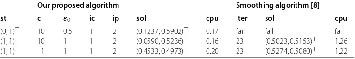
Table 3 Numerical results of Example 4.3
Our proposed algorithm Smoothing algorithm [8]
st c ε0 ic ip sol cpu iter sol cpu
(0, 1) 10 0.5 1 2 (0.1237, 0.5902) 0.17 fail fail fail
(1, 1) 10 1 1 2 (0.0590, 0.5236) 0.16 23 (0.5023, 0.5153) 1.26
(1, 1) 1 1 1 2 (0.4533, 0.4973) 0.20 23 (0.5274, 0.5080) 1.22
In our numerical experiments, the parameters used in the algorithm are chosen as fol-lows:σ= .,δ= .,μ= ,γ = .min{, /H(z)}. The algorithm terminates when ψ(zk) ≤–. In the tables of test results,stdenotes the starting point ofx,icdenotes the corrector iteration numbers in Step followed directly from Step ,ipdenotes the predictor iteration numbers,iterdenotes the iteration numbers of smoothing method (in []),cpudenotes the CPU time for solving the underlying problems in seconds, andsol denotes a solution of the test problem. In the following, we reveal a detailed description of the tested problems.
In the following, we reveal a detailed description of the tested problems. For Exam-ple ., . and ., we compare the results obtained by our method with which obtained by smoothing method []. The results are summarized in Table , Table and Table .
Example .[, ] Consider (.), wheref= (f,f)withx∈Rand
f(x) =x+x– , f(x) = –x–x+ (.).
Example .[, ] Consider (.), wheref = (f,f)withx∈Rand
f(x) =sin(x), f(x) = –cos(x).
Example .[] Consider (.), wheref = (f,f)withx∈Rand
[image:14.595.117.478.300.360.2]5 Conclusion
In this paper, we present a new smoothing and regularization predictor-corrector algo-rithm to solve the nonlinear inequalities, the global and local convergence are obtained. Furthermore, the smoothing parameterμand the regularization parameterεin our algo-rithm are viewed as independent variables. Preliminary numerical results show the effi-ciency of the algorithm.
Competing interests
We declare that we have no competing interests.
Authors’ contributions
The author carried out the proof. The author conceived of the study and participated in its design and coordination. The author read and approved the final manuscript.
Acknowledgements
This research was supported by the Natural Science Foundation of China (Grant Nos. 11171180, 11171193, 11126233, 10901096) and the fund of Natural Science of Shandong Province (Grant Nos. ZR2009AL019, ZR2011AM016). The authors are in debt to the anonymous referees for their numerous insightful comments and constructive suggestions which help improve the presentation of the article. The authors thank Prof. Yiju Wang for his careful reading of the manuscript.
Received: 14 July 2011 Accepted: 19 September 2012 Published: 2 October 2012 References
1. Zakian, V, Nail, UA: Design of dynamical and control systems by the method of inequalities. Proc. Inst. Electr. Eng.120, 1421-1472 (1973)
2. Dennis, JE, Schnabel, RB: Numerical Methods for Unconstrained Optimization and Nonlinear Equations. Prentice-Hall, Englewood Cliffs (1983)
3. Neumaier, A: Interval Methods for System of Equations. Cambridge University Press, Cambridge (1990) 4. Daniel, JW: Newtons method for nonlinear inequalities. Numer. Math.21, 381-387 (1973)
5. Mayne, DQ, Polak, E, Heunis, AJ: Solving nonlinear inequalities in a finite number of iterations. J. Optim. Theory Appl.
33, 207-221 (1981)
6. Sahba, M: On the solution of nonlinear inequalities in a finite number of iterations. Numer. Math.46, 229-236 (1985) 7. Yin, HX, Huang, ZH, Qi, L: The convergence of a Levenberg-Marquardt method for nonlinear inequalities. Numer.
Funct. Anal. Optim.29, 687-716 (2008)
8. Huang, ZH, Zhang, Y, Wu, W: A smoothing-type algorithm for solving system of inequalities. J. Comput. Appl. Math.
220, 355-363 (2008)
9. Zhu, JG, Liu, HW, Li, XL: A regularized smoothing-type algorithm for solving a system of inequalities with a P0-function. J. Comput. Appl. Math.233, 2611-2619 (2010)
10. He, C, Ma, CF: A smoothing self-adaptive Levenberg-Marquardt algorithm for solving system of nonlinear inequalities. Appl. Math. Comput.216, 3056-3063 (2010)
11. Huang, ZH, Qi, L, Sun, D: Sub-quadratic convergence of a smoothing Newton algorithm for theP0and monotone
LCP. Math. Program.99, 423-441 (2004)
12. Zhao, N, Huang, ZH: A nonmonotone smoothing Newton algorithm for solving box constrained variational inequalities with aP0function. J. Ind. Manag. Optim.7(2), 467-482 (2011)
13. Huang, ZH, Han, J, Chen, Z: Predictor-corrector smoothing Newton method, based on a new smoothing function, for solving the nonlinear complementarity with aP0function. J. Optim. Theory Appl.117, 39-68 (2003)
14. Herty, M, Klar, A, Singh, AK, Spellucci, P: Smoothed penalty algorithms for optimization of nonlinear models. Comput. Optim. Appl.37, 157-176 (2007)
15. Burke, J, Xu, S: A noninterior predictor-corrector path-following algorithm for the monotone linear complementarity problem. Math. Program.87, 113-130 (2000)
16. Luca, TD, Facchinei, F, Kanzow, C: A semismooth equation approach to the solution of nonlinear complementarity problems. Math. Program.75, 407-439 (1996)
17. Clarke, FH: Optimization and Nonsmooth Analysis. Wiley, New York (1983)
18. Mifflin, R: Semismooth and semiconvex functions in constrained optimization. SIAM J. Control Optim.15(6), 957-972 (1977)
19. Qi, L, Sun, J: A nonsmooth version of Newton’s method. Math. Program.58(3), 353-367 (1993)
20. Lee, YJ, Mangasarin, OL: SSVM: A smooth support vector machine for classification. Comput. Optim. Appl.20, 5-22 (2001)
21. Che, H, Li, M: A smoothing and regularization Broyden-like method for nonlinear inequalities. J. Appl. Math. Comput. (2012). doi:10.1007/s12190-012-0588-2
22. Chen, B, Harker, PT: A non-interior-point continuation method for linear complementarity problems. SIAM J. Matrix Anal. Appl.14, 1168-1190 (1993)
23. Huang, ZH, Han, J, Xu, D, Zhang, L: The non-linear continuation methods for solving the P0-functions non-linear complementarity problem. Sci. China44(2), 1107-1114 (2001)
24. Facchinei, F, Kanzow, C: Beyond monotonicity in regularization methods for nonlinear complementarity problems. SIAM J. Control Optim.37(2), 1150-1161 (1999)
26. Zhang, Y, Huang, ZH: A nonmonotone smoothing-type algorithm for solving a system of equalities and inequalities. J. Comput. Appl. Math.233, 2312-2321 (2010)
27. Qi, L, Sun, DF, Zhou, GL: A new look at smoothing Newton methods for nonlinear complementarity problems and box constrained variational inequalities. Math. Program., Ser. A87, 1-35 (2000)
doi:10.1186/1029-242X-2012-214