Binary classification algorithms

ORIGINAL RESEARCH ARTICLE

BINARY CLASSIFICATION ALGORITHMS

*Roumen Trifonov, Daniela Gotseva and Vasil Angelov

Faculty of Computer Systems and Technology, Technical University, Sofia 1000, Bulgaria

ARTICLE INFO ABSTRACT

The classification is a vital part of the Data mining process. It can be accomplished by different algorithms, divided into various groups. Those groups are based on machine learning techniques such as frequency tables, covariance matrices and other analytical statistical approaches. Each of the presented groups has its own advantages and disadvantages and therefore is applicable to a specific situation. The situation is determined by the objects that need to be classified into separate groups, also called object domains. Significant part of the domain cases is represented by two classes. This fact brings forward the need of defining binary classification.

*Corresponding author

Copyright ©2017,Roumen Trifonovet al. This is an open access article distributed under the Creative Commons Attribution License, which permits unrestricted

use, distribution, and reproduction in any medium, provided the original work is properly cited.

INTRODUCTION

Most of the practical cases include assigning a specific category or a class of appurtenance of an object. The task of classifying elements to one of two available groups is called binary or binomial classification. This task is executed according to a specific classification rule. Example of application of binary classifiers can be observed in the fields of:

 Computer science – spam filters for determining

whether particular email is spam or not, based on the subject’s description;

 Medicine – diagnosing patients if they have specific disease or not;

 Education – test evaluation – if the examinee has passed the test or not;

 Information retrieval – if a specific document should be included in a final result set or not.

The machine learning theory provides the theoretical apparatus for implementation of classification algorithms. Those algorithms include:

 Decision trees – part of the Frequency Table group;

 Support vector machines – part of the Covariance

Matrix group;

 Logistic regression – part of the Analytical group.

Some of the algorithms can be applied to classification of more than two classes, but the current article is focused on the binary classification aspect. The output of the classification algorithm is a prediction score, indicating the system’s “certainty” that the given object belongs to the positive class. In order to accomplish this, the implemented algorithm compares the score to a classification threshold. If the score is above the threshold the object is classified as positive class, respectively the instances with lower scores are classified as negative. Based on the classification the objects can be divided into four groups: true positive (correct positive predictions), true negative (correct negative predictions), false positive (incorrect positive predictions) and false negative (incorrect negative predictions). Those groups can be represented in table format, called confusion matrix (Figure 1). The elements at the main diagonal contains the correctly predicted objects (TP and TN) and the remaining objects are the wrongly classified ones (FP and FN).

ISSN: 2230-9926

International Journal of Development Research

Vol. 07, Issue, 11, pp.16873-16879, November,2017

Article History:

Received 17th _{August 2017} Received in revised form 08th September, 2017 Accepted 04th _{October, 2017} Published online 29th _{November, 2017}

Available online at http://www.journalijdr.com

Key Words:

Classification, Machine learning, Data mining, Class, Object, Decision tree (DT),

Support vector machines (SVM), Logistic regression.

Citation: Roumen Trifonov, Daniela Gotseva and Vasil Angelov,2017. “Binary classification algorithms”, International Journal of Development Research, 7, (11), 16873-16879.

Figure 1. Confusion matrix

There are additional indicators, based on those values. Using them the implemented algorithms can be evaluated for the specific application domain. The elements at the main diagonal contains the correctly predicted objects (TP and TN) and the remaining objects are the wrongly classified ones (FP and FN). There are additional indicators, based on those values. Using them the implemented algorithms can be evaluated for the specific application domain.

Classification Trees

Decision trees, also known as classification trees, represent one of the major groups of machine learning algorithms. The use of trees depicts the decision process in an intuitive way and therefore each classification chain (set of branches that lead from the root of the tree to the terminal node) can easily be interpreted. This approach mimics the way of thinking of the human’s brain.

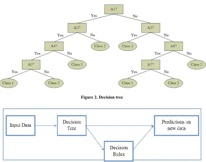
The tree depicts a discrete model of the outcome of the classification process. The discrete values are produced via inductive inference. The classification trees define information structures represented by instances in the format of attribute-value pairs. Each tree contains a finite number of attributes and each instance stores a value for the corresponding attribute. Each node of the tree corresponds to a specific test. The result of the test directs the output to one of the next nodes, connected to the tested one via branches. The steps of the analysis and classification process include executing the test on the nodes of the decision tree. Performing all the tests on the nodes down the tree from the root to one of the leaf nodes provides the classification of a specific instance. The node includes test of one of the attributes of the instance. The descending branches from the tested node represent the possible values of that attribute. The process of classifying instances starts with the test of the attribute of the root node and then moving down the tree branch that corresponds to the value of that attribute. This branch is connected to another node, containing test of another attribute. The process includes executing such tests and moving down the branches until a leaf node is reached. The discrete values in the output (the classified instances) are generated via target functions. The simplest case is observed with the Boolean classification – there are only two available classes for the classifier to assign to. The classification trees (depicted on Figure 2) can be reviewed as disjunctions of conjunctions of the limitations of the attributes’ values. Each route from the root to a leaf node corresponds to a conjunction of the values in each node/attribute. The complete tree contains the disjunction of all those conjunctions.

Figure 2. Decision tree

The construction of decision trees is performed by searching for irregularities in the available data. This article is focused on the ID3 algorithm by Ross Quinlan. The Iterative Dichotomiser 3 (ID3) algorithm is a predecessor of the C4.5 algorithm (also by Quinlan) and is considered to be the core algorithm in the field of decision trees construction

1997 and Winston, 1992).

The main ideas, incorporated in the ID3 algorithm are:

 The non-leaf nodes correspond to attributes. The

branches from each node point to a specific value of the attribute;

 A leaf node corresponds to the expected value of the output attribute when the input attributes are consistent with the path from the root to the that leaf node;

 Decision tree can be qualified as “good” when each path consists of nodes that have the most informative input attributes about the output attribute in the leaf node at the end the corresponding path. The idea behind that is the use of smallest set of ques

when predicting the output;

 The adoption of entropy from the field of information theory. The entropy measures how informative an input attribute is about the output attribute for the training data subset.

The ID3 algorithm implements top-down, greedy search in the space of possible branches without backtracking mechanism. In order to accomplish that, the most important moment of the ID3 algorithm is the selection of the tested attribute at specific node. This is performed via the statistical measurement, called information gain (IG). The IG measures the level of how given attribute separates the training set in correspondence with the target function. At any iteration of the decision tree generation, the IG is used to select suitable attribute for each node. Decision trees are built using the top-down approach, starting with the root. This technique includes partitioning the data into subsets, such as each subset contains instances with similar values. Those subsets are called homogenous. I

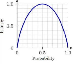
another statistical instrument, called entropy (E) to calculate the homogeneity of the subset sample (Figure 4). E = 0 when the sample is completely homogenous. If the sample is equally divided, then E = 1.

Figure 4. Entropy graph

The building of the decision tree requires the use of frequency tables. These tables contain each attributes and the number of its reoccurrence in the dataset. ID3 requires the calculation of two types of entropy for the set of examples S:

Entropy using the frequency table of one attribute

16875 International Journal of Development Research,

The construction of decision trees is performed by searching for irregularities in the available data. This article is focused on the ID3 algorithm by Ross Quinlan. The Iterative predecessor of the C4.5 algorithm (also by Quinlan) and is considered to be the core algorithm in the field of decision trees construction (Mitchell,

The main ideas, incorporated in the ID3 algorithm are:

spond to attributes. The branches from each node point to a specific value of the

A leaf node corresponds to the expected value of the output attribute when the input attributes are consistent with the path from the root to the that leaf node; Decision tree can be qualified as “good” when each path consists of nodes that have the most informative input attributes about the output attribute in the leaf node at the end the corresponding path. The idea behind that is the use of smallest set of questions on average

The adoption of entropy from the field of information theory. The entropy measures how informative an input attribute is about the output attribute for the training

down, greedy search in the space of possible branches without backtracking mechanism. In order to accomplish that, the most important moment of the ID3 algorithm is the selection of the tested attribute at specific cal measurement, called information gain (IG). The IG measures the level of how given attribute separates the training set in correspondence with the target function. At any iteration of the decision tree generation, bute for each node. down approach, starting with the root. This technique includes partitioning the data into subsets, such as each subset contains instances with similar values. Those subsets are called homogenous. ID3 uses another statistical instrument, called entropy (E) to calculate the homogeneity of the subset sample (Figure 4). E = 0 when the sample is completely homogenous. If the sample is equally

of the decision tree requires the use of frequency tables. These tables contain each attributes and the number of its reoccurrence in the dataset. ID3 requires the calculation of two types of entropy for the set of examples S:

table of one attribute

( ) = − log

where c is the number of available different values and p probability of one randomly selected example of S to belong to class i. The base of the logarithm is 2, because the entropy is a measurement of the expected length of encoding in bits and there are only two bits: 0 and 1. In this case the maximum value of the entropy is log2c.

Entropy using the frequency tables of two attributes:

( , ) = ( ) ( )

∈

where X is the set of available values, P(c) is the probability of selecting class c and E(c) is the entropy of that class’ a

For binary classification we have only two classes (positive and genitive in the general case) and therefore (1) can be transformed to:

( ) = − log − log

where p+ is the positive proportion of the examples in S set of

examples and p- is the negative proportion. If all the examples

in S belong to one of the classes (either positive, or negative), the entropy is 0. When the number of positive examples equals the number of negative examples, the entropy is 1. If the number of positive examples is not equal to the number of negative ones, then the entropy is between 0 and 1, as it is depicted on the Figure 4.

The IG is based on the decrease of the entropy after the partitioning of the dataset by a specific attribute. The construction of decision tree requires attribute with the highest IG, i.e. the most homogenous branches. In order to calculate the IG, the following steps have to be executed: the dataset is split on the different attributes. After that the entropy for each new subset is calculated. Then it is added proportionally, to get the total entropy for the split. After that the resulting entropy is subtracted from the entropy before the split. The result is the information gain (IG), representing the decrease in entropy:

( , ) = ( ) − ( , )

Then the attribute with the largest IG is selected to be the decision node and to divide the decision node by its branches. This process is repeated on every new branch. A branch with E = 0 is a leaf node and a branch with E more than 0 needs to be subjected on the aforementioned procedure i.e. needs further splitting. The ID3 algorithm is executed recursively on the non-leaf nodes until all the attributes have assigned tests on nodes in the tree. Once the decision tree is available, it can be transformed into a set of decision rules, because, by definition the classifications trees are disjunctions of decision rules. This can be achieved by mapping the nodes from the root to each leaf one after another. Each rule is a conjunction of attribute’s values, situated in the corresponding nodes.

Support Vector Machine (SVM)

This approach for classification uses a hyperplane for maximizing the margin between the two classes. The vectors (also known as cases) used for the hyperplane definition are the support vectors.

International Journal of Development Research, Vol. 07, Issue, 11, pp.16873-16879, November, 2017

………(1)

where c is the number of available different values and pi is the

probability of one randomly selected example of S to belong to class i. The base of the logarithm is 2, because the entropy is a measurement of the expected length of encoding in bits and there are only two bits: 0 and 1. In this case the maximum

Entropy using the frequency tables of two attributes:

……….(2)

where X is the set of available values, P(c) is the probability of selecting class c and E(c) is the entropy of that class’ attribute. For binary classification we have only two classes (positive and genitive in the general case) and therefore (1) can be

……….(3)

is the positive proportion of the examples in S set of is the negative proportion. If all the examples in S belong to one of the classes (either positive, or negative), the entropy is 0. When the number of positive examples equals er of negative examples, the entropy is 1. If the number of positive examples is not equal to the number of negative ones, then the entropy is between 0 and 1, as it is

The IG is based on the decrease of the entropy after the titioning of the dataset by a specific attribute. The construction of decision tree requires attribute with the highest IG, i.e. the most homogenous branches. In order to calculate the IG, the following steps have to be executed: the dataset is e different attributes. After that the entropy for each new subset is calculated. Then it is added proportionally, to get the total entropy for the split. After that the resulting entropy is subtracted from the entropy before the split. The result is the

nformation gain (IG), representing the decrease in entropy:

………(4)

Then the attribute with the largest IG is selected to be the decision node and to divide the decision node by its branches. ated on every new branch. A branch with E = 0 is a leaf node and a branch with E more than 0 needs to be subjected on the aforementioned procedure i.e. needs further splitting. The ID3 algorithm is executed recursively on the ttributes have assigned tests on Once the decision tree is available, it can be transformed into a set of decision rules, because, by definition the classifications trees are disjunctions of decision rules. This g the nodes from the root to each leaf one after another. Each rule is a conjunction of attribute’s values, situated in the corresponding nodes.

Support Vector Machine (SVM)

This approach for classification uses a hyperplane for maximizing the margin between the two classes. The vectors (also known as cases) used for the hyperplane definition are

This does not require previous knowledge for the problemati area. SVM performs great with large scale datasets (Theodoridis, 2003). Let us have two available classes. can be separated by multiple planes with zero error rates (as it is depicted in Figure 5). But what about the additional classes – they may or may not be divided correctly by a randomly selected hyperplane from the available ones. The classifier needs to select one plane, based on the assumption how good it will classify the remaining “hidden” test examples (Figure 6).

Figure 5. SVM with multiple hyperplanes

Figure 6. SVM with optimal hyperplane

Let us have N training examples. Each examples is defined by the pair <xi, yi> (i = 1, 2, …, N), where xi = (x

and yi ∈ {-1, 1}. The solutions for linear classifier can be

presented with model’s parameters w and b in the form of:

⃗ ∙ ⃗ + = 0 ………..

For the examples that belong to the solution (marked as x xb) plane we have:

⃗ ∙ ⃗ + = 0 ……….

w⃗ ∙ x ⃗ + b = 0 ………..

If we subtract these equations ((6) – (7)) we have:

⃗ ∙ ( ⃗ − ⃗) = 0 ……….

16876 Roumen Trifonov

This does not require previous knowledge for the problematic area. SVM performs great with large scale datasets Let us have two available classes. They can be separated by multiple planes with zero error rates (as it is depicted in Figure 5). But what about the additional classes may not be divided correctly by a randomly selected hyperplane from the available ones. The classifier needs to select one plane, based on the assumption how good it will classify the remaining “hidden” test examples (Figure 6).

multiple hyperplanes

SVM with optimal hyperplane

Let us have N training examples. Each examples is defined by = (xi1, xi2, …, xid)

1, 1}. The solutions for linear classifier can be presented with model’s parameters w and b in the form of:

………..(5)

For the examples that belong to the solution (marked as xa and ……….(6)

………..(7)

(7)) we have: ……….(8)

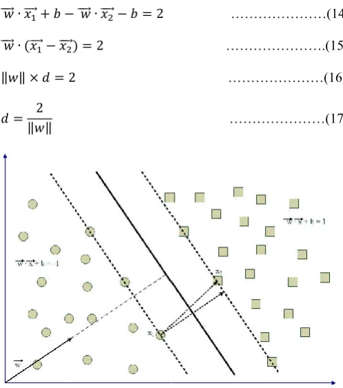
where ( ⃗ − ⃗) is a parallel to the solution plane, directed vector from xa to xb. Because the dot product is 0, the direction of ⃗ is perpendicular to the solution plane. For each instance xs above the solution plane is true: ⃗ ∙ ⃗ + = , ℎ > 0 and for each instance xc below the solution plane is true: ⃗ ∙ ⃗ + = ′_{, ℎ} ′_{< 0} If we denote all instances above the plane with +1 and all instances below the plane with y of each test example z, we have the following general rule: = +1, ⃗ ∙ ⃗ + > 0 −1, ⃗ ∙ ⃗ + < 0 Once we define the linear classifier, we can maximize the available classification margin by changing the parameters w and b. The margin is represented by two parallel hyperplanes bi1 and bi2: ∶ ⃗ ∙ ⃗ + = 1 ∶ ⃗ ∙ ⃗ + = −1 The margin is actually the distance between these two hyperplanes. In order to determine the distance, let us assume that x1 is point on bi1 and x2 is a point on b points in the equations, the distance d can be calculated by the subtraction of the second from the first equation (Figure 7): ⃗ ∙ ⃗ + − ⃗ ∙ ⃗ − = 2 ⃗ ∙ ( ⃗ − ⃗) = 2 ‖ ‖ × = 2 = 2 ‖ ‖ Figure 7. SVM - distance between two different instances The learning phase of the SVM algorithm includes the evaluation of the parameters w and b order to satisfy the following conditions: ⃗ ∙ ⃗ + ≥ 1, oumen Trifonov et al. Binary classification algorithms is a parallel to the solution plane, directed . Because the dot product is 0, the direction is perpendicular to the solution plane. For each instance above the solution plane is true: ………(9)

below the solution plane is true: ………...(10)

If we denote all instances above the plane with +1 and all instances below the plane with -1, for the value of the attribute y of each test example z, we have the following general rule: ……….(11)

Once we define the linear classifier, we can maximize the available classification margin by changing the parameters w and b. The margin is represented by two parallel hyperplanes ………(12)

………(13)

The margin is actually the distance between these two hyperplanes. In order to determine the distance, let us assume is a point on bi2. Replacing the points in the equations, the distance d can be calculated by the subtraction of the second from the first equation (Figure 7): ………(14)

……….(15)

………(16)

………(17)

⃗ ∙ ⃗ + ≤ −1, = −1 ………...(19)

Due to the restrictions of the position of the classes (the first class instances (class 1) have to be on or above the top hyperplane and the second class instances (class -1) have to be on or below the second hyperplane), we have the second form for representation:

( ⃗ ∙ ⃗ + ) ≥ 1, ∀ , = 1, 2, … , …………...(20)

There is additional requirement for the SVM algorithm – the available margin has limit, called maximum hyperplane margin and it is:

min‖ ‖

2 ℎ ( ⃗ ∙ ⃗ + ) ≥ 1, ∀ ,

= 1, 2, … , …………(21)

Due to Quadratic nature of the function and the linear restrictions for w and b, this task is known as convex optimization problem. One of the advantages of the SVM is that if the input data set is linearly separable, then there exists a unique global minimum value.

The ideal case is when the SVM produces a hyperplane that separates the classes completely without overlapping. But this may not always be possible, as it is depicted on Figure 8 – there are two instances that are on the other side of the hyperplane. In this case the SVM finds hyperplane that will maximize the margin and minimize the misclassification. If there is an example that is situated in the margin, it may be misclassified. In order to minimize the misclassification we need to introduce a slack variable. This variable allows some instances to fall off the margin, but adds penalties to them. The SVM algorithm works to maintain the slack variable as close to zero as possible while the margin is maximal. The main equation (20) needs to be recalibrated in the following form:

( ⃗ ∙ ⃗ + ) ≥ 1 − , ∀ , ≥ 0, = 1, 2, … , ……(22)

Figure 8. SVM with ovelaping instances

The penalty for the margin can be introduced with the following formula:

min‖ ‖

2 + ………….(23)

C is a user-defined parameter for the misclassification penalty of the tested examples. Two groups of data can be separated by one line (in the case of one dimension), a flat plane (two

dimensions) or an N-dimensional hyperplane

(multidimensional space). But there are more cases and situations where non-linear curve can separate the groups more efficiently. This can be accomplished by a kernel function to map the data into the correct space. This can be reviewed as a non-linear function that is being learned by a linear learning machine in a high-dimensional space. Meanwhile the capacity of the system can be controlled by a parameter that is not dependable on the space’s dimensionality. This is also known as kernel trick and the kernel function transforms the dataset into a higher dimensional space in order to make it possible to perform the linear separation.

Logistic Regression

The Logistic Regression model is applicable for binary classification or prediction when we have only two possible

outcomes – positive/negative, yes/no, pass/fail,

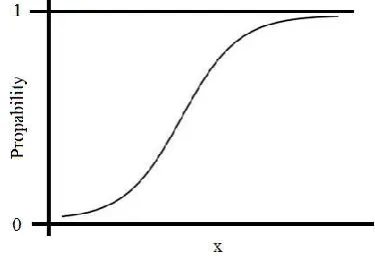
class_1/class_2, etc. There are cases with more than two outcome categories, which are analyzed via multinomial logistic regression, but this article is focused exclusively on the binomial case. To predict means to assign a value on an instance, i.e. to classify that instance in one class. The prediction process is based on specific dependent variables called predictors. The number of those predictors can be one or many and their type can be numerical or categorical. The logistic regression generates a logistic curve with values between 0 and 1 (Figure 9). The curve is constructed via natural logarithm of the “odds” of the targeted variable instead of the probability [5]. There is no need for the normal distribution of the predictors in each group. The logistic regression is also known as logit regression or logit model.

Figure 9. Logistic regression curve

The Logistic Model can be represented with the following equation:

= 1

1 + ( ) ………(24)

The constant b0 translates the slopes on the abscissa (x-axis)

and the b1 defines the curve’s steepness. We can transform the

equation in terms of the odds ratio:

1 − =

( ) _{……….(25)}

By using the natural logarithm we ca rewrite (25) in logarithmic form, the so called log-odds or logit form:

ln = + ………….(26)

This form of the equation represents the predictors by a linear function. The coefficient b1 represents the change in the logit

with change of x with one unit.

The Logistic Regression can work with multiple numerical or categorical variables. In that case the equation needs to be transformed to:

= 1

1 + ( ⋯ ) ………..(27)

The regression model needs to be evaluated and in order to accomplish that we need to measure the model adequacy. This can be performed with the squared multiple correlation indices, called pseudo R2 indices [2]. It assesses the goodness of fit in the predictive model. There are several pseudo R2 variants. The first one is Lave and Efron’s pseudo R2, calculated by the equation:

= 1 −∑ ( − )

∑ ( − ) ……….(28)

where p is the logistic model predicted probability and n is the number of observations in the model. The model residuals are squared, summed, and divided by the total variability in the dependent variable.

Other variant is the McFadden’s pseudo R2, defined by the following equation:

= 1 − ………..(20)

The ratio of the log-likelihoods suggests the level of improvement over the intercept model offered by the full model. In order to adjust the model we can include penalty for the number of predictors (k):

= 1 − − ………(21)

Another index, described by Maddala, Cox and Snell that also reflects the likelihood (but not log-likelihood) functions of the intercept and the full models is:

= 1 − ………(22)

Due to the possibility of exceeding the value of 1.0, there is another pseudo R2 index proposed by Cragg and Uhler and Nigelkerke:

= 1 −

1 −

………..(23)

Another variation of the index is the count pseudo R2 that is equal to the accuracy of the prediction model:

= ………….(24)

There is also an adjusted from of (24) that takes into consideration the count of the most frequent outcome (N):

= −

− ……...(25)

There is a likelihood ratio test which is used to compare the goodness of fit of two models: one of the models, called intercept or null model, is a special case of the other, called full model. It tests the significance of the distance between the likelihood ratios for the full model minus the one for the null model. This difference is also known as “model chi-square (Chi2)”. The likelihood ratio test provides the ability to compare the logarithmic variants of the likelihood of two different models (one is complete and the other is restricted):

= ln( ) + (1 − ) ln(1 − ) ………(26)

where p is the predicted probability of the logistic model. Then we have to calculate the doubled difference of between the log-likelihoods of the two competing models:

2( − ) ………(27)

To test the significance of each individual predictor in the model is used Wald test (like prediction contribution). The Wald test is used to evaluate the statistical significance of the b coefficients:

= − ~ (0,1) ………(28)

where W is the Wald's statistic with a normal distribution, b is the coefficient and SE is its standard error. If we square this equation the squared standard normal distribution is the chi-square distribution with one degree of freedom ( ):

= − ~ ……….(29)

Usually the parameter of interest b0 = 0 and therefore the Wald

statistics test can be reduced to the estimate of the coefficient divided by its standard error:

= ~ (0,1) ………..(30)

Conclusion

The presented classification algorithms belong to the field of machine learning, but their productive use in the data mining classification process is undeniable. Some of the algorithms can be used in classification that implements prediction of more than two outcome classes. The decision trees present the outcome of the classification in easy to comprehend way, due to the self-explanatory nature of the tree structure. The visual depiction of the classified instances of the SVM and logistic regression methods is also easy to understand and to review in consequential analysis.

REFERENCES

Mitchell, T. 1997. Machine Learning. McGraw-Hill, pp. 52-78.

Smith, T., McKenna, C. 2013. A Comparison of Logistic Regression Pseudo R2 Indices. Multiple Linear Regression Viewpoints, Vol. 39 (2), pp. 19-26.

Theodoridis, S., Koutroumbas, K. 2003. Pattern Recognition. Second Edition, Elsevier, pp. 55-88.

Winston, P. 1992. Artificial Intelligence. Addison-Wesley Publishing, pp. 423-442.

Witten, I, Frank, E., Hall, M. 2011. Data Mining – Practical Machine Learning Tools and Techniques. Third Edition, Morgan Kaufmann Publishers, pp. 125-127

*******