3003
A REVIEW OF CONSTRUCTIVE INTERFERENCE
FLOODING IN WIRELESS SENSOR NETWORKS
HUDA A. H. ALHALABI1,TAT-CHEE WAN2
1 Postdoctoral Fellow, Universiti Sains Malaysia, National Advanced IPv6 Centre,
11800 USM, Penang, Malaysia
2 Associate Professor, Universiti Sains Malaysia, National Advanced IPv6 Centre /
School of Computer Sciences, 11800 USM, Penang, Malaysia E-mail: 1[email protected], 2[email protected]
ABSTRACT
Constructive interference is a promising concurrent transmission technique for multiple senders concurrently transmitting the same packet in wireless sensor networks. It enables reliable and fast network flooding in order to decrease the scheduling overhead of MAC protocols, improve link quality of lossy links, achieve accurate time synchronization, and to realize efficient data collection. This paper discusses the concept of constructive interference, its importance, pre-conditions and open issues and challenges that should be considered by the researchers. This paper delivers the knowledge about constructive interference in WSN as a literature review, to get more knowledge about this emerging technique.
Keywords: Constructive Interference, Wireless Sensor Networks, Flooding, Concurrent Transmissions, Synchronization
1. INTRODUCTION
Conventional wireless communication systems consider packet collisions as a problem and try to avoid them by using techniques like channel reservations, carrier sense, or arbitrated medium access (TDMA, polling). The intuition is that concurrent transmissions make packet transmission undecodable and cause irretrievable bit errors at the receiver. However, researchers have found that this view is too conservative. The researchers have proved that the packets can still be decoded successfully at the receiver despite collisions, if the signal of interest power exceeds the sum of interference from colliding packets by a certain threshold, the stronger signal is received and decoded. This effect, referred to the capture effect
[1], has been validated in many practical studies on different communication systems such as IEEE 802.15.4 [2]– [3] and IEEE 802.11 [4]– [5]. Recently, researchers have explored that it is probable for some or all packets in a collision to survive. There are opportunities to improve the network throughput, increase the overall channel utilization, if we design protocols that select terminals carefully for transmitting simultaneously [6], [7]. The concurrent transmission benefits are not just of theoretical interest but have been verified practically and implemented in application
3004 Proposed time Scheduling mechanisms for data collection are described in Section 5. Section 6 discusses open issues and challenges. Comparisons and Evaluation are presented in Section 7, and finally the conclusion presented in Section 8.
2. CONSTRUCTIVE INTERFERENCE When multiple transmitters send the same packet to a common receiver simultaneously, interference between the concurrent transmitted packets is constructive if it helps the common receiver to decode the original signal correctly. By contrast, interference is destructive if it prevents the common receiver from decoding the superimposed signals accurately. Figure 1 shows that CI requires the identical waveforms being transmitted within a threshold period Tc. In fact, the period Tcdescribes
[image:2.612.325.514.331.442.2]the physical layer tolerance for multi-path signals. If the maximum temporal displacement Δ exceeds the threshold period, the receiver may not be able to decode the packet correctly. This results in destructive interference [19].
Figure 1: Concurrent Transmissions of an Identical Packet with IEEE 802.15.4 Radio
Constructive interference (CI) is a physical layer phenomenon and was first discovered experimentally by Dutta et al. [9] who used CI in backcast to avoid broadcast storm problem. A backcast is a link-layer exchange frame, in which a single radio frame triggers zero or more acknowledgment frames that interfere at the initiator non-destructively. Figure 2 shows a backcast frames involving three nodes. The backcast exchange begins with the initiator transmitting a probe frame to the hardware broadcast address. The two responders automatically transmit identical acknowledgments. These two acknowledgments interfere at the initiator, if certain conditions are met, this interference is non-destructive, allowing the initiator to decode the acknowledgment frame correctly, and conclude that at least one of its
neighbors responded. Constructive interference (CI) is a physical layer phenomenon and was first discovered experimentally by Dutta et al. [9] who used CI in Backcast to avoid broadcast storm problem. A Backcast is a link-layer exchange frame, in which a single radio frame triggers zero or more acknowledgment frames that interfere at the initiator non-destructively. Figure 2 shows a Backcast frames involving three nodes. The Backcast exchange begins with the initiator transmitting a probe frame to the hardware broadcast address. The two responders automatically transmit identical acknowledgments. These two acknowledgments interfere at the initiator, as long as certain conditions are met, this interference is non-destructive, allowing the initiator to decode the acknowledgment frame correctly, and conclude that at least one of its neighbors responded.
Figure 2: A Backcast Exchange Involving Three nodes
Exploiting CI in wireless networks is a rising trend, for it allows multiple senders transmit the same packet simultaneously. CI- based flooding can achieve millisecond network flooding latency and sub-microsecond time synchronization accuracy, adapt to topology changes and require no network state information [19]. The following are the main CI benefits in WSNs:
- CI can alleviate the ACK storm problem as employed in Backcast [8].
- Reduce the transmission latency of acknowledge packets [19].
[image:2.612.96.296.359.493.2]3005 constructive interference depends on the communication scheme. Glossy first reviewed the IEEE 802.15.4 modulation, and then derive the max temporal displacement among multiple concurrent packet transmissions to be received with high probability. Figure 3 shows a simple CI-based generated signal at a base station.
Figure 3: Generating CI from Coherently Added Signals
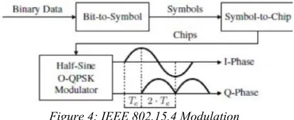
The IEEE 802.15.4 node is operating in the 2.4 GHz band. The data to be sent is first divided into 4-bit groups each creating a symbol. Each symbol goes through a Direct Sequence Spread Spectrum (DSSS) modulation. Each symbol is modulated with a pseudo-random noise (PN) sequence of 32 chips. The symbol-to-chips mapping is determined in the IEEE 802.15.4 standard [21]. This baseband signal is then modulated to the carrier with Offset-Quadrature Phase Shift Keying (O-QPSK), which is transmitted over the wireless medium. At the receiver, a coherent detection method is used to demodulate the carrier signal. The signal is down-converted into chips, which are then mapped back to the symbols using Maximum Likelihood Estimation (MLE). PN sequence introduce redundancy allows for coping up with errors caused by the channel or soft-decisions at chip-level. This redundancy improves the receiver sensitivity level at the cost of reduced data rate. For CI to occur, the maximum temporal displacement between received signals is 0.5 μs [11], since the chips on quadrature phase (Q-phase) are delayed by the chip time Tc = 0.5 μs from the in-phase (I-phase) carrier. As mentioned in [19], let the O-QPSK signal be represented by,
(1)
Here, I(t) is the I-phase, Q(t) is the Q-phase component, and ωc =pi/2Tc is the radial frequency
of half-sine pulse wave. The resulting signal of the constructive interference is given by,
(2)
where, K is the number of concurrent transmitters, Ai is the amplitude and τi is the temporal offset of the ith transmitted signal. Ni(t) is the noise added to the signal. Figure 4 illustrates the IEEE 802.15.4 modulation.
Figure 4: IEEE 802.15.4 Modulation
Wilhelm et al. [19] show that thus network flooding protocols, such as Glossy, should aim to keep the transmission time error Tc < 250 ns to ensure a desired PRR above 75%. If Tc < 200 ns can be ensured, the achievable PRR is approximately 90%. 2.2 Sufficient Conditions for generating CI Wang et al. [14] derived theoretical sufficient conditions (SC) for concurrent transmissions with IEEE 802.15.4 radio to interfere constructively. i) Concurrent transmissions with the same packet must be synchronized at chip level, namely less than Tc=0.5μs.
ii) The phase offset of the ith received signal should satisfy:
≤ -1 (3)
Where Pi is the average power of the ith received signal, P1 is the average power of the strongest
signal.
iii) The ratio of the minimum signal to noise ratio (SNR) 𝜆 min and the maximum SNR λmax of concurrent transmissions should satisfy:
≥ (4)
3. Time Synchronization
When using the CI technique, it is of greatest importance to respect time synchronization in the transmission of simultaneous packets. According to [11], time displacement between multiple packets should be less than 0.5μs, half of the DSSS chip duration in IEEE 802.15.4.
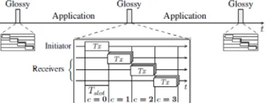
3.1 Glossy
[image:3.612.108.269.193.291.2]3006 This triggers other nodes to receive and relay the packet. Glossy benefits from this fast-concurrent packet transmissions from a source node (initiator) to all other nodes (receivers) in the network. After the first transmission of the initiator, the flooding process is entirely driven by radio events. For instance, a node triggers a transmission only if the packet reception completed. Although the concurrent transmissions of glossy are fast and synchronized implicitly, they must be properly aligned to enable a receiver to decode the packet successfully. The radio driven execution of glossy is a key factor to meet this requirement. It inserts into each packet a 1-byte field, the relay counter c. Before the first transmission the initiator sets c = 0. Nodes increment c by 1 before relaying a packet. Consequently, a node can guess from the relay counter how many times a received packet was relayed, as shown in the lower part of figure 5. We define the slot length Tslot as the time between the start of packet transmission with relay counter c and the start of the next packet transmission with relay counter c+1. Using timestamps of the radio interrupts, nodes locally estimate Tslot. Tslot is a network-wide constant, since nodes never change the packet length during a flood. To achieve accurate time synchronization, the initiator embeds its own clock value into the flooding packet, and all nodes who receive from the initiator synchronize their clocks to this reference time.
Figure 5: Glossy Decouples Flooding from Other Application Tasks Executing on the Nodes
The time required by the main Glossy states depends mostly on the radio hardware. The MCU influences the timing only after the packet reception complete, or to trigger a packet transmission by MCU, this small period is called the software delay
Tsw, and it is affected by the communication between the radio and MCU. Tslot which is an
important property to achieve high synchronization accounts for the software delay Tsw,
the transmission time Ttx, and the radio processing
delay Tdat the beginning of a packet reception. Tslot
can thus be expressed as:
Tslot = Tsw + Ttx + Td (5)
3.2 Triggercast
Triggercast as proposed by Wang et al. [23] is a practical distributed middleware to generate CI in
WSNs. It enables a co-sender to trigger a radio signal, which acts as a common reference for all concurrent transmitters to establish a synchronized transmission. Triggercast uses Glossy flooding; besides it proposed a chip level synchronization (CLS) to compensate the radio processing delays in order to have 0.5μs synchronized concurrent transmission.
In the MAC layer, the trigger node uses a standard CSMA/CA protocol to acquire the medium. Once the trigger node senses a free channel, it first broadcasts a synchronization packet, and informs the destination to all the co-senders and when to start sending data. After a little duration of time, all the co-senders start to transmit simultaneously. In the PHY layer, Triggercast uses the proposed chip level synchronization (CLS) and link selection and alignment (LSA) algorithms to guarantee synchronized transmitted packets interfere constructively. For receiver-initiated Triggercast, the receiver first runs LSA to select best links to join the concurrent transmissions. As illustrated in figure 6, for sender-initiated Triggercast, each co-sender individually performs the LSA, to determine whether it will participate in the concurrent transmission process. Then selected senders use CLS to evaluate propagation and radio processing delays. Finally, they run a number of no operations (NOPs) to compensate the measured delays and phase offsets found in LSA.
Figure 6: Triggercast: A Radio Triggered Concurrent Transmission Architecture
4. Impact Factors
Wilhelm et al. [20] concludes the main factors that may influence the probability of a successful reception under interference, as following:
[image:4.612.324.517.453.543.2]3007 This model can be applied if the adding signals are uncorrelated. However, when the interfering signals are correlated, this model is not accurate and further factors should be considered [24], [25], [26].
2. Signal timing: In packet radios, the signal power alone is not sufficient for successful reception. The relative timing of colliding packets significantly affects the reception process; if the stronger signal arrives the receiver later, it disturbs the first packet reception, and both colliding packets are lost. Therefore, the receiver should be synchronized and locked onto the captured signal. Many researches analyze possible collision patterns and their effect on packet reception [26] and propose a new receiver scheme that releases the lock when a stronger signal arrives, discards the first packet and accepts the second one, the so-called message-in-message (MIM) capture [25], [27].
3. Channel coding: the bit-level coding is also an influence factor on packets reception success. For example, in DSSS systems a set of b bits is encoded into a longer sequence of B chips [28], in order to increase the resilience to interference; since the receiver can cross-correlate the chipping sequences, to filter out any encoded noise. However, DSSS systems require uncorrelated interfering signals such as signals without coding or with orthogonal chipping sequences to get their theoretical coding gain. Another possibility is to have a delay capture [29] when there is an adequate time offset between interfering packets with the same coding.
4. Packet contents: The length and content of packets also affect the reception performance of colliding packets. For instance, Dutta et al. [9] show that short collided packets can be received with a PRR over 90%, thus enabling the design of an efficient receiver-initiated link layer. Similarly, the latency of flooding protocols of WSNs can be significantly reduced [11]. These insights show that packet and capture synchronization alone are not enough to explain the performance of these protocols, and bit-level modeling that also includes content and signal timing is necessary.
5. Carrier phase: For the phase modulated signals, knowledge of the carrier phase at the receiver is essential for successful reception; because the data is carried in the phase variations of the signal [28]. Classically, the phase offsets are minimized during the synchronization phase of packet reception. Existing capture models have reduced phase offsets. However, their models are not sufficient; because of two reasons, first, in novel protocols exploiting packet collisions, the preamble synchronization is not always able to succeed. Second, there are other new applications of
concurrent transmissions that try to neglect the synchronization procedure. For example, Pöpper et al. [18] study the possibility of manipulating separate message bits on the physical layer and conclude that carrier phase offsets are the major difficulty to do so reliably.
6. Number of Concurrent Interferers: The
experimental performance of Glossy shows no noticeable dependency on node density. However, theoretically performance and node density are not independent.
Maheshwari et al. [41] noticed that the SIR value is not varying with an increasing number of interferers. Lu and Whitehouse [12] observed a decreasing PRR when the number of interferers is increased. However, the Flash Flooding protocol depends on capture, such that increased time offsets may also manipulate the results. Some related work claims that a larger number of concurrent interferers cause problems (Doddavenkatappa et al.
[10], Wang et al. [13]) because “the probability of the maximum time displacement across different transmitters exceeding the required threshold for constructive interference” might increase. Gezer et al. [2] show that the PRR decreases with an increasing number of interferers.
[image:5.612.347.491.572.686.2]Yu et al. [37] show that the number of transmitters (M) is a critical parameter in the design of concurrent transmission. On one hand, the advantage of constructive interference is not obvious if M is too small. On the other hand, the benefit from constructive interference is limited and too much overhead is introduced if M is too large. Yu et al. approved that PRR can be significantly improved by exploiting CI. Nevertheless, as node number increases, the growth rate of PRR decreases. As shown in figure 7, when node number exceeds 6, the enhancement of PRR is trivial. This may be because the maximum temporal displacement Δ of concurrent transmissions becomes closer to Tc when node number increases.
3008 5. TIME SCHEDULING MACHANISMS
LWB [19], Chaos [30], and Choco [31] build up level scheduling mechanism for dissemination or data collection based on Glossy.
5.1 Low-Power Wireless Bus (LWB)
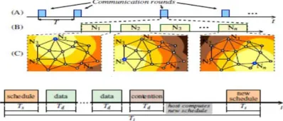
[image:6.612.321.519.97.166.2]The LWB protocol sits between radio driver and application, and totally replaces the standard network stack. LWB maps all Glossy floods communications. A single flood serves to broadcast a packet from one node to all other nodes. To avoid collisions between different floods, LWB adopts a time-triggered operation: a global communication schedule determines when a node is allowed to initiate a flood. LWB exploits the global time synchronization of Glossy. The protocol operation is limited within communication rounds. As shown in figure 8 (A), rounds are repeated every round period T which is computed at the host and can vary relying on the current traffic demands. In order to save energy, nodes keep their radios off between two rounds. Each round consists of a number of non-overlapping communication slots, as shown in figure 8 (B). In each slot, at most one node initiates a flood (puts a message on the bus) whereas all other nodes receive the message on the bus and relay the flood, as shown in figure 8 (C). All nodes join in every flood. Figure 8 shows the communication slots of one round of length Tl. A round starts with a slot of length Ts allocated to the host for distributing the communication schedule. Using this schedule, the nodes time-synchronize with the host and to be up-to-date of (i) the round period T and (ii) the mapping of source nodes to the data slots of length Td. A non-allocated contention slot of length Td follows; this slot may be used by nodes to report the host of their traffic demands. The host uses these to add the schedule for the next round, when it transmits an ending slot of length Ts. The host determines a new communication schedule by computing a proper round period T and allocating data slots to the current streams. A stream characterizes a traffic demand, represented by a starting time and an inter-packet interval (IPI), as LWB targets the periodic traffic pattern of many low power wireless applications [32], [19].
Figure 8: Time-Triggered Operation in LWB
Figure 9: Communication slots within a round
LWB is proposed as an efficient scheduler for Glossy. It is topology agnostic, which doesn’t need to spend time and energy in building routing tables. However, LWB doesn’t perform any data aggregation; it just uses each flood to collect single node’s information. Thus, LWB considered as a collection protocol, which can be improved to have the benefits of aggregation [33].
5.2 Chaos
Chaos [20] is a synchronous all-to-all data aggregation protocol, based on flooding. Chaos only enables computing aggregates that are both decomposable and duplicate-agnostic. Chaos works on two mechanisms: i) Leveraging the capture effect [29] through tight synchronization, and ii) A coordinating structure, called the flags field. Fig. 9 illustrates how Chaos works. There are three main phases; Initialization, Aggregation and Termination.
- Initialization: At the beginning of the round, nodes turn on their radios, setup their flags by setting only the bit associated with their id and set their local aggregate same as their initial. The resulting state of the packets can be seen in slot 0 of figure 9. Next, all nodes except one, wait and listen to the channel for an incoming packet. That special node that performs the first transmission is called the initiator.
- Aggregation: Once the nodes receive a Chaos message, they update their flags-fields and aggregated values. If the flags of the nodes change, they broadcast the updated information directly after the processing step ends. In figure 9, as soon as receiving the message from A in slot 1, nodes B and C update their flags-field, so it shows that they now have node A's information. After that, they simultaneously transmit their updated messages in slot 2. The tight synchronization of Chaos enables all receivers to transmit their updated packets at the same time, basically causing synchronized collisions. Then by leveraging the capture effect, the information of these collisions can be decoded.
[image:6.612.96.295.639.724.2]3009 flags. It then stops the aggregation and broadcasts its final information.
Synchronization in Chaos: In Chaos, both round and slot synchronization are achieved. Slot synchronization is quite simple: after the reception of a packet, which ends at the same time for all nodes, nodes create a highly deterministic timeout to reach the determined length of the processing step. When this timeout occurs, an interrupt is triggered, and nodes send their own data. Round synchronization is more complex and requires: i) the knowledge of the slots number passed from the first transmission and ii) the slot length. Chaos is able to acquire this information by timing communication events and using the hop count field of a packet [33]. The key limitation of Chaos is that it relies on processing. When receive a packet, the nodes process its payload and flags to the merge operator, which takes significantly longer time than glossy.
5.3 Choco
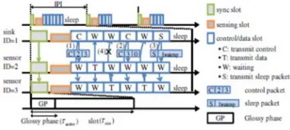
Choco [31] presents a slot scheduler and low-power controller upon Glossy. A sink node schedules slots for each node taking into account traffic and packet losses of the nodes. Also, the sink determines a Low power control. Nodes with Choco communicate in a slotted form as shown in figure 10. A sink node periodically broadcasts time synchronization packets using Glossy to synchronize all the nodes in the network. A slot has a length of τslot, and at most one Glossy phase with the duration of τactive is setting up at the beginning of the slot. The sink node allocates slots in a fine-grained and centralized manner considering each node’s traffic. Concretely, the sink node employs a slot schedule and transmits a control packet carrying the schedule for the network just before the actual communication. Figure 10 illustrates the sink node transmits a control packet after the sensor nodes complete their sensing tasks ((1) in figure 10). A control packet contains the schedule up to the payload length permitted by Glossy. The schedule determines which node is the owner of each slot in which the control packet is transmitted. In figure 11, the length of the payload is set to two. Once the schedule is completed, the sink node transmits a new control packet ((2) in figure 10) or a sleep packet ((3) in figure 10), depending on whether packets exist to be delivered to the sink. In Choco, there are three modes for sensor nodes: transmitting, waiting, and sleep mode. Each node determines its mode based on the current schedule information in the control packet. If the current slot is its own, a node enters transmit mode and become the initiator in Glossy. The initiator transmits a
[image:7.612.317.522.220.312.2]packet at the beginning of the slot. If the current slot is not its own, a node will be in the waiting mode. In case of losing a control packet, the node stays in waiting mode until the following control packet reception. A node in the waiting mode considered as a receiver in Glossy. When a node receives a sleep packet, each node goes into a sleep mode until the following control slot. In sleep mode, a node turns off the radio and set its timer to wakeup to receive the next control packet.
Figure 10: Slot assignment using control packets
The above time scheduling mechanisms achieve low duty cycle and efficient network flooding. However, they do not basically change the Glossy transmission mechanism, which brings unnecessary energy consumption.
6. OPEN ISSUES AND CHALLENGES
The open issues and challenges for successful CI in WSNs, which can be served as research topics for future work, are summarized in this section. 6.1 Energy Consumption
Glossy is emerging as a high reliability and latency optimal flooding technique. Then a question arises: is Glossy energy efficient? Unfortunately, Glossy makes all nodes participate in the data forwarding, which directly triggers huge number of excessive data transmissions, and leading to high energy consumption and network life reduction. This is a very critical issue; especially in energy limited large-scale WSNs. One efficient solution is to reduce redundant transmissions, while maintaining the benefits of CI-based flooding [34].
6.1.1 Forwarder Selection mechanism
3010
Figure 11: CX Forwarder Selection for Collection Traffic
Figure 11 shows how this mechanism works. For a node w to decide whether it can forward or not, it should know its distance from the destination, its distance from the source, and the distance from source to destination (ddw, dsw, and dsd,
respectively). In the case of data collection, the network root both sends out periodic TDMA schedule packets, and the destination for all data traffic. The schedule packets provide ddw to each potential forwarder and dsd to each potential source. The Burst Setup packet includes dsd and allows nodes to measure dsw (under the assumption of symmetric distances), and then make a forwarding decision for (s, d) packets. In the Data Forwarding phase, the nodes that have not been selected turn off their radios, and s transmits packets with interpacket spacing determined by dsd.
6.1.2 Energy Adaptive CI-based flooding
CI-based flooding is a network flooding approach based on the hierarchical model. In the first round, the initiator propagates a packet to its one-hop neighbors. Then, the one-hop neighbors will relay the received packets to the initiator and the two-hop neighbors in the second round. Every other round, nodes on each layer forward the flooding packet once. Each node stops forwarding packet if its transmission count reaches the transmission threshold.
CI-based flooding key factors are listed in Table 1.
𝑇𝑥 represents the node that begins to send a packet and 𝑅𝑥 is the particular event of receiving packet. When the flooding starts, only the initiator can transmit packet. Let SF𝑖 represents the node that becomes an initiator and SF𝑟 represents the node that becomes a receiver. SF𝑖 and SF𝑟 events are only triggered at the start of the network flooding process. Stop is the external event that stops the network flooding. 𝐶_𝑡𝑥 is the transmission counter which counts the number of transmissions of the current node. 𝑁_𝑡𝑥 is the transmission threshold.
[image:8.612.319.519.107.211.2]𝑅𝑥_𝑓 indicates that the node fails in receiving a packet. 𝑐 is the relay count which will be increased by one after every successful reception.
Table 1: The key Factors of CI-based Flooding
Cheng et al. [34] propose a distributed energy adaptive CI-based flooding protocol (EACIF) for WSNs. It uses Active Node Selection (ANS) method to reduce the number of active nodes set via the communication between neighbors. EACIF establishes a power consumption model for CI-based flooding and then analyzes the energy saving by EACIF in 𝑘-covered UDG.
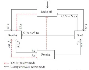
Figure 12: Node’s State Transition Graph for CI-Based Flooding
As figure 12 shows, CI-based flooding has four main states including Radio off, Standby, Send, and
Receive state. When SF𝑖 event occurs, the initiator transforms from Radio off into Send state. Then the initiator triggers the 𝑇𝑥 event to transmit a flooding packet to its one-hop neighbors. When SF𝑟 event happens, the nodes except the initiator switches to the Standby state and wait for the incoming packets. When 𝑅𝑥 event happens, the node go into Receive
state and begins to decode the received packet. If the reception is successful, ++𝑐 is performed, while the node shifts to Send state for new round of transmitting. In contrast, if 𝑅𝑥_𝑓 happens (Δ ≥ 0.5
𝜇s) the node transforms to the Standby state for the next receiving round. When 𝑇𝑥 event happens, the node has two candidate states: the Standby and the
Radio off state. If 𝐶_𝑡𝑥 is less than 𝑁_𝑡𝑥, the node will turn to Standby state to wait for the new 𝑅𝑥
event. If 𝐶_𝑡𝑥 equals 𝑁_ 𝑡𝑥, the node will switch to
[image:8.612.326.515.310.458.2]3011 CC2420 [44]. The energy consumption of Send and
Receive state is at milliampere level, while Radio off and Standby state only consume microampere-level. Clearly, the nodes should be at Radio off and
Standby states most of the time. Glossy, as a topology independent CI-based flooding protocol, employs all nodes in WSNs circling in Standby →
[image:9.612.94.279.230.330.2]Receive → Send until flooding completed. Each cycle has two “milliampere-level” states and one “microampere-level” state.
Table 2: Energy Consumption of CC2420 Radio
As figure 12 shows, each node in EACIF has two primary modes: the active mode and the passive mode. In active mode, the node has the same schedule with Glossy, while the node in passive mode need not forward the received packet. If it received the packet successfully, the node turns to
Radio off state to save energy. If the reception was unsuccessful, the node turns to Standby state for the next 𝑅𝑥 event. Obviously, the more nodes in passive mode, the more energy are saved.
6.1.3 Point-to –Point Packet Exchange
Jeong et al. [36] proposed PEASST (Point-to-Point Packet Exchange with Asynchronous Sleep and Synchronous Transmissions), a topology-free protocol that leverages concurrent transmissions to lower the cost of end-to end data transmission. PEASST integrates a receiver-initiated duty-cycling mechanism to reduce energy consumption, it designs a point-to-point transfer protocol that performs asynchronous radio duty-cycling and at the same time achieves the benefits of synchronous packet transmissions. PEASST sits between the application and radio driver to replace the network stack. The data transmission process in PEASST has three phases (1) selective network-wide wake up, (2) rapid flood-based packet delivery, and (3) sleep phase. In contrast to Glossy where all nodes in the network need to participate in the flooding session, PEASST aims to reduce this number of transmitting nodes to improve the network energy efficiency. Also, PEASST supports multiple point-to-point traffic flows in the network by eliminating the contention between concurrent flood sessions.
6.2 Scalability
Glossy exploits CI by quickly broadcasting a packet from the sink node to all other nodes in the entire network. The time slot Tslot between each hop
contains the duration for data reception and retransmission. The slot relies on the packet length and thus is a network-wide constant. Although, Glossy achieves near-optimal flooding latency, it is difficult to keep precise timing for large number of concurrent transmitters in practice. τe is defined as
the time uncertainty during the time slot Tslot in
each hop. In Glossy, τe is described by the clock
uncertainty τtx due to clock frequency drifts during
the packet transmission, the radio processing uncertainty τd, the propagation delay uncertainty τp
and the statistical uncertainty of the software delay τsw. Therefore, it can be expressed as:
τe = τsw+τd +τtx+τp (4)
After packet transmission through h hops, the maximum accumulated time displacement Δ among simultaneous transmissions to a common receiver is expected to exceed the threshold period Tc. In addition, as the number of transmitters m increase, the probability that the maximum time displacement Δ exceeds the threshold period Tc
also increase. That indicates that CI-based flooding suffers the scalability problem. In other words, as the size or the density of a wireless network grows, the precondition ΔTc may not hold, resulting in packet collisions.
In Eq. (4), τp can be perfectly removed when
accurate node localization is enabled. The software delay uncertainty τsw represents the additional deviation due to the unsynchronized clocks of the MCU and the radio. Accordingly, τsw is a discrete
random variable with granularity 1/ fr, where fr =
8MHz is the radio clock frequency. It should be observed that τsw can be eliminated with the new generation chips e.g. cc2530, integrating radio modules and MCU in one chip with synchronized clock frequency. Caused by the offset between the asynchronous radio clocks of the transmitter and the receiver, the radio processing uncertainty τdis a
random variable with uniform distribution in the interval [0;1/fr]. Clock uncertainty τtx, during a
packet transmission, results from the clock frequency drifts, which are due to aging effects and temperature.
In [43], the frequency drift ρ related to the nominal frequency fo can be modeled as a Gaussian variable
with distribution N (0; δ2 ρ). It is reasonable to assume ρ is constant during a packet transmission time Tslot. Therefore, the clock uncertainty τtxdue to
3012 (6)
As a result, the probability mass function (pmf) of the time uncertainty τeper hop can be calculated as
the convolution of the pmfs of the independent
random variables. For
a path of h hops, the pmf
pe of accumulated
time uncertainty τhecan be obtained by
(7) For m independent paths, each of which consists h
[image:10.612.114.289.388.508.2]hops originated at the sink node; the maximum temporal displacement Δ is defined as. The calculation of cumulative distribution function (CDF) of Δ corresponds to the problem of finding the CDF of the range of m independent identically distributed random variables. This is a well-known order statistics problem, and the pmf has been shown in [42]. Figure 13 illustrates the CDF of the maximum temporal displacement Δ when the density or the size of the network of worst case varies. From Fig. 13, it can be noticed that the CDF with m = 5; h = 6 is only 50%, which is intolerable for system design.
Figure 13: CDF versus Δ of different h (m = 5;N = 1)
The performance of Glossy depends on the network size. Flooding latency L and radio on time T increase linearly on the maximum hop distance between initiator and receivers. While flooding reliability R decreases logarithmically, as the network size increases [11].
Wang et al. [23] show that Glossy has a scalability problem. The PRR of Glossy is inversely proportional to the independent paths’ hops. That because the independent paths increase cumulative synchronization errors.
6.2.1 Spine CI- based Flooding
Wang et al. [23] proposed SCIF (Spine
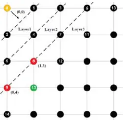
Constructive Interference based Flooding) protocol, which utilizes grid topology to reduce the number of independent paths. They first construct a spine of a given topology through an automatic spine node
[image:10.612.360.481.391.509.2]selection process. Then implement network flooding on the spine in the same way as Glossy. Different from Glossy, if the nodes in SCIF do not belong to the spine, they should only receive the packets, without retransmitting them again, to construct the grid spine, they divide the area into several grid cells, and post a CellID ((4; 4), e.g.) for each cell. Each node in the network decides which cell it belongs to, based on its geometric location. In each cell there will be at most one node as the spine node. Therefore, nodes of the same cell compete to become a spine node within an automatic process. In this process, a node firstly broadcasts a message to ask whether there is a spine node in this cell. If not, the node waits for a specific amount of time and announces itself as the spine node for its cell [3]. Fig. 14 shows a CI- based network flooding process in a simple 4x4 grid topology. At first, the sink node N0 broadcasts a packet to one hop slave nodes N1 and N2 at layer 1. After nodes N1 and N2 receive the packet, they forward the packet simultaneously to nodes at layer 2 and so forth. In view of node 13, its PRR equals to the CDF of maximum temporal displacement of packet transmissions between its parent nodes N8 and N9.
Figure 14: Constructive Interference Based Flooding in a 4x4 Grid Topology
low-3013 latency are significant system features. Nevertheless, this study exposes a critical lack of link quality scalability with the number of concurrent forwarders [22].
6.3 Latency
Recently, CI- based flooding is emerging as a latency optimal flooding technique. As a representative CI- based flooding protocol, Glossy achieves millisecond level flooding latency which is almost 100 times faster than conventional flooding solutions [39, 40]. Yu et al. [37] propose
Constructive Interference-based
Reliable Flooding (CIRF), which design a reliable flooding in asynchronous duty-cycle WSNs. CIRF is integrated with the MAC protocol Receiver-Initiated (RI-MAC) to improve the utilization of wireless medium and ensure one-hop reliable transmission. The main idea of CIRF is to exploit the CI feature when concurrent transmission occurs, using RI-MAC based WSNs. CIRF approach efficiently reduces latency and energy costs. 6.3.1 Tree Pipelining
Doddavenkatappa et al. [10] proposed Splash, a new data dissemination protocol, which eliminates contention overhead by exploiting CI. Splash achieves high scalability to large, multi-hop sensor networks and it relies on two recent works: Glossy and PIP (Packets in Pipeline) [38]. It forms fast parallel pipelines by exploiting channel diversity and constructive interference. Splash was designed based on PIP’s approach that includes three key contributions to support data dissemination to many receivers over multiple paths:
1. Tree pipelining which use constructive interference to successfully create parallel pipelines over multiple paths that cover all the nodes in a network. For this purpose, a collection tree is utilized in the reverse direction for dissemination, which in turn helps to mitigate the scalability problem of CI and to eliminate the differences that exist among different channels performance. 2. Opportunistic overhearing from peers by using multiple pipelines, which provides more chances of receiving a packet to each node.
3. Channel cycling that raises the chance of reutilizing a good channel, as well as avoiding interference. Different channels are used at several stages of the pipeline between various transmission rounds to avoid stalling of the pipeline when a bad channel is accidentally chosen. Figure 15 illustrates the tree pipelining.
7. COMPARISON AND EVALUATION
To have an efficient approach which utilizes CI in WSNs, three main aspects should be considered;
energy consumption, latency and scalability. Most of the proposed approaches have focused on one issue over other vital issues. Regarding latency, Glossy, EACIF, and Splash achieve the lowest network latency. However, all of them suffer the scalability problem. Splash can realize higher throughput than Glossy.
Figure15: Illustration of Pipelining Over a Tree
On the other hand, repeated channel switching increases the cumulative synchronization error, and thus decreases accuracy and reliability. In addition, channel scheduling increases energy consumption. EACIF can reduce energy consumption since it reduces the number of active nodes via ANSA algorithm. However, PRR of Glossy is higher than in EACIF, that because EACIF reduces the retransmission and reduces opportunities to attain the packets. However, EACIF seems to be the most energy efficient approach. CXFS, SCIF and PEASST are the most scalable approaches since they reduce the transmitting nodes. Nevertheless, their processes increase the network latency. CXFS selection method reduces the number of nodes to save energy, while it costs considerable computational overhead, which also consumes high energy. The grid topology of SCIF improves the flooding scalability; but it increases the path length of CI-based flooding and so increases the network latency. According to the discussed issues and previous works, researchers can benefit from the CI-Flooding by designing protocols that selects the transmission nodes carefully, to eliminate the displacement error and improve PRR in a large network to solve the problem of scalability. Also, reducing the number of transmitting nodes can save energy and decrease the network latency. Table 3 and 4, summarize the main CI approaches and compare between them based on energy efficiency, scalability and latency.
3014 network flooding latency and sub-microsecond time synchronization accuracy. This paper discusses the fundamental concept of CI and reviewed the state- of -art of different research exploiting it. All the reviewed approaches are improving WSNs’ performance using CI. Nevertheless, they have limitations on network efficiency such as high energy consumption, scalability problem or increase network latency. Therefore, more work is needed to improve the performance of the whole wireless sensor network while employing CI. The main advantage of CI-Flooding is that it improves network connectivity and reliability of the network. However, the key limitation of this approach is the high energy consumption of the flooding nodes. As a future work, an efficient clustering and selection algorithms can be employed in the WSN to select best relays to cooperate in the CI-Flooding, to improve the connectivity and reliability while reducing the energy consumption and maximizing the network lifetime.
REFERENCES
[1] K. Leentvaar and J. Flint, “The capture effect in FM receivers,” IEEE Trans. Commun., vol. 24, pp. 531–539, May 1976.
[2] C. Gezer, C. Buratti, and R. Verdone, “Capture effect in IEEE 802.15.4 networks: Modelling and experimentation,” in Proc. IEEE ISWPC ’10,pp. 204–209, May 2010.
[3] D. Son, B. Krishnamachari, and J. Heidemann, “Experimental study of concurrent transmission in wireless sensor networks,” in
Proc. ACM SenSys ’06, pp. 237–250, Nov. 2006.
[4] J. Foo and D. Huang, “Multiuser diversity with capture for wireless networks: Protocol and performance analysis,” IEEE J. Sel. Areas Commun., vol. 26, pp. 1386–1396, Oct. 2008. [5] J. Lee, W. Kim, S.-J. Lee, D. Jo, J. Ryu, T.
Kwon, and Y. Choi, “An experimental study on the capture effect in 802.11a networks,” in
Proc. ACM WinTECH ’07, pp. 19–26, Sept. 2007.
[6] M. Sha, G. Xing, G. Zhou, S. Liu, and X. Wang, “C-MAC: Model driven concurrent medium access control for wireless sensor networks,” in
Proc. IEEE INFOCOM ’09, pp. 1845–1853, Apr. 2009.
[7] M. Vutukuru, K. Jamieson, and H. Balakrishnan, “Harnessing exposed terminals in wireless networks,” in Proc. USENIX NSDI ’08, pp. 59–72, Apr. 2008.
[8] P. Dutta, S. Dawson-Haggerty, Y. Chen, C.-J. M. Liang, and A. Terzis, “Design and
evaluation of a versatile and efficient receiver-initiated link layer for low-power wireless,” in
Proc. ACM SenSys ’10, pp. 1–14, ACM, Nov. 2010.
[9] P. Dutta, R. Musaloiu-E., I. Stoica, and A. Terzis, “Wireless ACK collisions not considered harmful,” in Proc. ACM SIGCOMM HotNets-VII, pp. 4:1–6, Oct. 2008. [10] M. Doddavenkatappa, M. C. Chan, and B. Leong, “Splash: Fast data dissemination with constructive interference in wireless sensor networks,”in Proc. USENIX NSDI ’13, pp. 269–282, Apr. 2013.
[11] F. Ferrari, M. Zimmerling, L. Thiele, and O. Saukh, “Efficient network flooding and time synchronization with Glossy,” in Proc. IPSN ’11,pp. 73–84, Apr. 2011.
[12] J. Lu and K. Whitehouse, “Flash Flooding: Exploiting the capture effect for rapid flooding in wireless sensor networks,” in Proc. IEEE INFOCOM ’09, pp. 2491–2499, Apr. 2009. [13] Y. Wang, Y. He, X. Mao, Y. Liu, and X. Li,
“Exploiting constructive interference for scalable flooding in wireless networks,”
IEEE/ACM Trans. Netw., vol. 21, pp. 1880– 1889, Dec. 2013.
[14] Y. Wang, Y. Liu, Y. He, X.-Y. Li, and D. Cheng, “Disco: Improving packet delivery via deliberate synchronized contructive interference,”IEEE Trans. Parallel Distrib. Syst., 2014.
[15] D. Wu, C. Dong, S. Tang, H. Dai, and G. Chen, “Fast and fine-grained counting and identification via constructive interference in WSNs,” in Proc. IEEE/ACM IPSN ’14, pp. 191–202, Apr. 2014.
[16] N. Santhapuri, S. Nelakuditi, and R. R. Choudhury, “On spatial reuse and capture in ad hoc networks,” in Proc. IEEE WCNC ’08, pp. 1628–1633, Apr. 2008.
[17] D. Davis and S. Gronemeyer, “Performance of slotted ALOHA random access with delay capture and randomized time of arrival,” IEEE Trans. Commun., vol. 28, pp. 703–710, May 1980.
[18] C. Pöpper, N. O. Tippenhauer, B. Danev, and S. ˇCapkun, “Investigation of signal and message manipulations on the wireless channel,” in Computer Security – ESORICS 2011, no. 6879 in LNCS, pp. 40–59, Springer, Sept. 2011.
[19] F. Ferrari, M. Zimmerling, L. Mottola, and L. Thiele, “Low power wireless bus,” in
3015
Embedded Networked Sensor Systems (SenSys ’12), pp. 1–14, November 2012.
[20] M. Wilhelm, V. Lenders, and J. Schmitt “On the Reception of Concurrent Transmissions in Wireless Sensor Networks,” IEEE Trans Commun.,vol.13, no.12 , pp. 6756-6767 , Dec. 2014.
[21] IEEE. std. 802.15.4-2003, 2003.
[22] C. Noda, M. C. Pérez-Penichet, B. Seeber, M. Zennaro, M. Alves, and A. Moreira. "On the scalability of constructive interference in low-power wireless networks." In Wireless Sensor Networks, pp. 250-257. Springer International Publishing, 2015.
[23] Y. Wang, Y. He, D. P. Cheng, Y. Liu, and X. Li, “Triggercast: enabling wireless constructive collisions,” in Proceedings of the IEEE INFOCOM, Turin, Italy, April 2013.
[24] R. Gummadi, D. Wetherall, B. Greenstein, and S. Seshan, “Understanding and mitigating the impact of RF interference on 802.11 networks,” in Proc. ACM SIGCOMM ’07, pp. 385–396, Sept. 2007.
[25] J. Lee, W. Kim, S.-J. Lee, D. Jo, J. Ryu, T. Kwon, and Y. Choi, “An experimental study on the capture effect in 802.11a networks,” in
Proc. ACM WinTECH ’07, pp. 19–26, Sept. 2007.
[26] N. Santhapuri, S. Nelakuditi, and R. R. Choudhury, “On spatial reuse and capture in ad hoc networks,” in Proc. IEEE WCNC ’08, pp. 1628–1633, Apr. 2008.
[27] K. Whitehouse, A. Woo, F. Jiang, J. Polastre, and D. Culler, “Exploiting the capture effect for collision detection and recovery,” in Proc. IEEE EmNetS-II, pp. 45–52, May 2005. [28] J. Proakis and M. Salehi, Digital
Communications. New York, NY: McGraw-Hill, 5th ed., Nov. 2007
[29] D. Davis and S. Gronemeyer, “Performance of slotted ALOHA random access with delay capture and randomized time of arrival,” IEEE Trans. Commun., vol. 28, pp. 703–710, May 1980.
[30] O. Landsiedel, F. Ferrari, and M. Zimmerling, “Chaos: versatile and efficient all-to-all data sharing and in-network processing at scale,” in
Proceedings of the 11th ACM Conference on Embedded Networked Sensor Systems, p. 1, ACM, November 2013
[31] M. Suzuki, Y. Yamashita, and H. Morikawa, “Low-power, end-to-end reliable collection using glossy for wireless sensor networks,” in
Proceedings of the 77th Vehicular Technology Conference (VTC ’13), pp. 1–5, June 2013.
[32] A. Mainwaring et al. “Wireless sensor networks for habitat monitoring”. In 1st ACM Intl. Workshop on Wireless Sensor Networks and Applications (WSNA ’02).
[33] D. Chronopoulos. "Extreme Chaos: Flexible and Efficient All-to-All Data Aggregation for Wireless Sensor Networks." PhD diss., TU Delft, Delft University of Technology, 2016. [34] D. Cheng, M. Yanyan, W. Yin , and W.
Xiangrong. "Improving energy adaptivity of constructive interference-based flooding for WSN-AF." International Journal of Distributed Sensor Networks, p.6, 2015.
[35] D. Carlson, C. Mingchao, T. Andreas,C. Yin, and G. Omprakash. "Forwarder selection in multi-transmitter networks." In Distributed Computing in Sensor Systems (DCOSS), IEEE International Conference on, pp. 1-10. 2013. [36] J. Jeong, P. Jongjun, J. Hoon Jeong, M. L.
Chieh-Jan, and K. JeongGil. "Low-power and topology-free data transfer protocol with synchronous packet transmissions." In Sensing, Communication, and Networking (SECON), Eleventh Annual IEEE International Conference on, pp. 399-407. 2014.
[37] Sh. Yu, W. Xiaobing, W. Pan,W. Dingming, D. Haipeng, and Ch. Guihai. "CIRF: Constructive interference-based reliable flooding in asynchronous duty-cycle wireless sensor networks." In Wireless Communications and Networking Conference (WCNC), IEEE, pp. 2734-2738. 2014.
[38] B. Raman, K. Chebrolu, S. Bijwe, and V. Gabale. PIP: A Connection-Oriented, Multi-Hop, Multi-Channel TDMA based MAC for High Throughput Bulk Transfer. In
Proceedings of SenSys, 2010.
[39] F. Stann, J. Heidemann, R. Shroff, and M. Z. Murtaza, “RBP: robust broadcast propagation in wireless networks,” in Proceedings of the 4th International Conference on Embedded Networked Sensor Systems (SenSys ’06), pp. 85–98, Boulder, Colo, USA, October 2006. [40] T. Zhu, Z. Zhong, T. He, and Z. Zhang,
“Exploring link correlation for efficient flooding in wireless sensor networks,” in
Proceedings of the 7thUSENIXConference onNetworked Systems Design and Implementation (NSDI ’10), p. 4, San Jose, Calif, USA, April 2010.
3016 [42] B. Arnold, N. Balakrishnan, and H. Nagaraja,
“A first course in order statistics”. Society for Industrial Mathematics, vol. 54, 2008.
[43] Z. Zhong, P. Chen, and T. He, “On-demand time synchronization with predictable accuracy,” in Proceedings of IEEE INFOCOM, Shanghai, China, Apr. 2011.
3017
Table 3: CI main Approaches, Contributes, Features and Lacks
Table 4: Comparison Between CI Approaches based on Energy efficiency, Scalability and Latency
Approach Authors, year Contribution Features Lacks
Backcast Dutta et al, 2009 Discover CI experimentally. Solve Backcast
storm problem High loss ratio if the transmitting nodes more than two.
Glossy Ferrari et al, 2011 The first exploits CI of IEEE
802.15.4 symbols. High Reliability. Fast synchronized flooding.
High Energy consumption. Scalability problem.
Triggercast Wang et al, 2013 Introduce a sufficient condition for CI. Propose Triggercast.
Increase PRR. Increase latency and consume more energy
SCIF Wang et al, 2013 Propose spine CI- flooding protocol using grid topology.
Improve PRR Increase latency.
CXFS Carlson et al, 2013 Propose forwarder selection
mechanism Save energy Increase latency.
CIRF Yu et al, 2014 Propose a reliable
CI-flooding. Reduce latency and consume energy
Scalability problem
PEASST Jeong et al, 2014 Design Point-to-Point
Packet Exchange Protocol. Improve the energy efficiency Increase Latency. Packet loss probability.
Splash Doddavenkatappa et al ,2013
It forms fast parallel pipelines by exploiting channel diversity and CI.
Reduce latency
Improve scalability
Increase energy consumption.
EACIF Cheng et al, 2015 Proposes a distributed active
nodes selection. Reduce energy consumption Reduce latency
PRR value decrease when the network size increases.
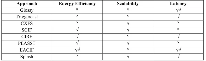
Approach Energy Efficiency Scalability Latency
Glossy ˟ ˟ √√
Triggercast ˟ ˟ √
CXFS ˟ √ ˟
SCIF √ √ ˟
CIRF √ ˟ √
PEASST √ √ ˟
EACIF √√ ˟ √√
[image:15.612.94.520.555.681.2]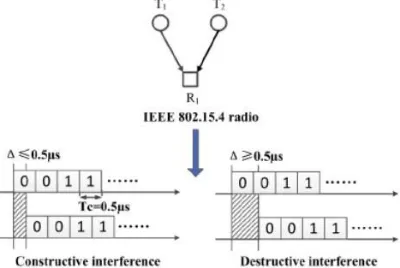
![Figure 7: PRR versus number of nodes [37]](https://thumb-us.123doks.com/thumbv2/123dok_us/8898010.953819/5.612.347.491.572.686/figure-prr-versus-number-of-nodes.webp)