STUDY OF SPI FRAMEWORK FOR CMMI CONTINUOUS MODEL BASED ON QFD

GLOWWORM SWARM OPTIMIZATION FOR

OPTIMIZATION DISPATCHING SYSTEM OF PUBLIC

TRANSIT VEHICLES

1_{YONGQUAN ZHOU,}2_{QIFANG LUO,} 3_{JIAKUN LIU} 1

Prof., College of Information Science and Engineering, Guangxi University for Nationalities, Nanning Guangxi 530006 P. R. China

2_{Assoc. Prof., College of Information Science and Engineering, Guangxi University for Nationalities,}

Nanning Guangxi 530006 P. R. China

3_{Master, College of Information Science and Engineering, Guangxi University for Nationalities, Nanning}

Guangxi 530006 P. R. China

E-mail: [email protected], [email protected]

ABSTRACT

The intelligent schedule of vehicles operation is one of the problems which need to be solved in the dispatching system of public transit vehicles, it relates to the development of the city and civic daily life. In this paper, a transit vehicle scheduling model which balancing between the benefits of bus companies and passengers is proposed. The glowworm swarm optimization (GSO) with random disturbance factor, namely R-GSO is applied to the schedule of vehicles. Comparing with classic swarm intelligence algorithms, the simulation results show our algorithm has higher efficiency and is an effective way to optimize the public transit vehicle dispatching.

Keywords: Public Transit Vehicle Dispatching, Glowworm Swarm Optimization (GSO), Random

Disturbance Factor.

1. INTRODUCTION

The scheduling problem is a classical multi-objective optimization question and dispatching system of public transit vehicles’ optimization is an actual problem [1]. To design the reasonable and convenient road network planning according to the urban traffic actual situation, work out the reasonable and effective urban public transport vehicle scheduling list considering social, bus company benefits. The current study of transit operation is divided into two methods. One is to adopt the simulation model, optimized the objective fitness function constructing by the simulation model. The other is to apply some operational research theory established the mathematical model, and then using intelligent algorithm to solve [2-5], [14-15]. Dispatching system of public transit vehicles is defined target for nonlinear optimization problem. It still has a lot of problems such as multi-objective function weights are difficult to be determined, the raw datasource is not accurate, and the algorithm convergence is insufficient ideal, etc.

Glowworm swarm optimization (GSO) [6-10] is a new method of swarm intelligence based algorithm for optimizing multi-modal functions

proposed by Krishnanad K. N. and Ghose D. in 2005. This algorithm becomes a new research hotspot of computational intelligence draw our sights on it. With the research deeper and deeper, it’s been used at noisy text of sensor and simulating robots. This paper introduces the basic GSO and glowworm swarm optimization with random disturbance factor, namely R-GSO, then applied them to the schedule of vehicles. The experimental results show that the improved algorithm can get better effect in the convergence and calculation.

This paper is organized as follows. In Section 2, a basic glowworm swarm optimization is proposed. In Section 3, we will introduce our glowworm swarm optimization with random disturbance factor for dispatching system of public transit vehicle, followed by the experimental results and analysis in Section 4. The conclusions are given in Section 5.

2. GLOWWORM SWARM OPTIMIZATION

has the respective field of vision scope called local decision range. Their brightness concerns with in the position of objective function value. The brighter the glow, the better is the position, namely has the good target value. The glow seeks for the neighbor set in the local-decision range, in the set, a brighter glow has a higher attraction to attract this glow toward this traverse, and the flight direction each time different will change along with the choice neighbor. Moreover, the local-decision range size will be influenced by the neighbor quantity, when the neighbor density will be low, glow’s policy-making radius will enlarge favors seeks for more neighbors, otherwise, the policy-making radius reduces. Finally, the majority of glowworm return gathers at the multiple optima of the given objective function.

Each glowworm

i

encodes the object function

value J x t

(

_i

( )

)

at its current location x t_i

( )

into a

luciferin value

l

_i

(

t

)

and broadcasts the same within its neighbourhood. The set of neighbours N t_i

( )

of

glowworm

i

consists of those glowworms that have a relatively higher luciferin value and that are located within a dynamic decision domain and updating by formula (1) at each iteration.

Local-decision range update:

|)}}

)

(

|

(

)

(

,

0

max{

,

min{

)

1

(

t

r

r

t

n

N

t

r

_di

+

=

_{s d}i

+

β

_t

−

_i

(1)

where

r

_di

(

t

+

1)

is the glowworm

i

’s

local-decision range at the t+1iteration,

r

s is the sensor

range,

n

_t is the neighbourhood threshold, the parameter

β

affects the rate of change of the neighbourhood range.

The number of glow in local-decision range:

)}

(

)

(

;

||

)

(

)

(

:||

{

)

(

t

j

x

t

x

t

r

l

t

l

t

N

i j

i d i

j

i

=

−

<

<

(2)

where,

x

_i

(

t

)

is the glowworm

i

’s position at the

titeration,

l

_i

(

t

)

is the glowworm

i

’s luciferin at the titeration.; the set of neighbours of glowworm

i

consists of those glowworms that have a relatively higher luciferin value and that are located within a dynamic decision domain whose range i

d

r is bounded above by a circular sensor range

s

r

(0

<

r

_di

<

r

_s

)

.Each glowworm

i

selects a

neighbour j with a probability p_ij

( )

t and moves toward it. These movements that are based only on local information, enable the glowworms to partition into disjoint subgroups, exhibit a simultaneous taxis-behavior toward and eventually co-locate at the multiple optima of the given objective function.

Probability distribution selects a neighbour:

∑

∈

−

−

=

) (

(

)

(

)

)

(

)

(

)

(

T N

k k i

i j ij I

t

l

t

l

t

l

t

l

t

p

(3)

Movement update:

















−

−

+

=

+

||

)

(

)

(

||

)

(

)

(

)

(

)

1

(

t

x

t

x

t

x

t

x

s

t

x

t

x

i j i j i

i (4)

Luciferin-update:

))

(

(

)

1

(

)

1

(

)

(

t

l

t

J

x

t

l

_i

=

−

ρ

_i

−

+

γ

_i (5)

and

l t

i

( )

is a luciferin value of glowworm i at the

t

iteration,

ρ

∈

(0,1)

leads to the reflection of the cumulative goodness of the path followed by the glowworms in their current luciferin values, the parameter

γ

only scales the function fitness

values, J x t

(

_i

( )

)

is the value of test function.

Each glowworm

i

selects a neighbour j with a

probability p_ij

( )

t and moves toward it. These

movements that are based only on local information, enable the glowworms to partition into disjoint subgroups, exhibit a simultaneous taxis-behaviour toward and eventually co-locate at the multiple optima of the given objective function.

The basic GSO algorithm as follows [6]:

Set number of dimensions

=

m

；

Set number of glowworms

=

n

；

Let

s

be the step size；

Let

x

i

(

t

)

be the location of glowworm

i

at time t；

Deploy_agents_randomly;

For

i

=

1

to n do

l

_i

(

0

)

=

l

₀

o i

d

r

r

(

0

)

=

Set maximum iteration number = iter_max;

{

For each glowworm

i

do :％Luciferin-update phase

l

_i

(

t

)

=

(

1

−

ρ

)

l

_i

(

t

−

1

)

+

γ

J

(

x

_i

(

t

))

; ％See(1)

For each glowworm

i

do : ％Movement-phase {

)};

(

)

(

);

(

)

(

:

{

)

(

t

j

d

t

r

t

l

t

l

t

N

_i

=

_ij

<

_di _i

<

_j

For each glowworm

j

∈

N

i

(

t

)

do;

( ) ( ) ( ) ( ) ( ) ( ) i j i ij k i

k N t

l t l t p t

l t l t ∈

− =

−

∑

; ％See(2)

=

j

select_glowworm

(

p



);

















−

−

+

=

+

)

(

)

(

)

(

)

(

*

)

(

)

1

(

t

x

t

x

t

x

t

x

st

t

x

t

x

i j i j i

i ; ％See(3)

)}}

)

(

(

)

(

,

0

max{

,

min{

)

1

(

t

r

r

t

n

N

t

r

_di

+

=

_{s d}i

+

β

_t

−

_i

％See(4)

}

t

←

t

+

1

:

}

Implementation at the GSO at the individual agent level gives rise to two major phases at the group level: Formation of dynamic networks that results in splitting of the swarm into sub-swarms and local convergence of glowworms in each subgroup to the peak locations.

3. PUBLIC TRANSIT VEHICLES DISPATCHING BY R-GSO

In order to avoid glowworm swarm optimization into the local optimal, give it the ability to expand the search scope, explore new areas. We insert the random disturbance factor at the movement update stage, and the formula as below:

randn

t

x

t

x

t

x

t

x

s

t

x

t

x

i j i j i

i





+

∗













−

−

+

=

+

σ

||

)

(

)

(

||

)

(

)

(

)

(

)

1

(

(6)

where randna random number in is [ 1,1]− , σ is the weighting factor of random disturbance.

In a public transport vehicle scheduling system [11], the bus route length is L having M bus stations. Bus companies operating time

is

[

time time

_m

,

_n

]

, and divided intoK stages, the

[1,

]

k

∈

K

interval is

∆

t

_k. Suppose in the route of the public transport vehicles on the same model, running at the same rate, arrive on time, each station passengers to obey the uniformly distributed, the bus fare passengers each of the same. From two aspects, the bus company earnings and passengers waiting time, according to one day each site and operation conditions of the passenger flow, solving the route of the vehicle running schedule.

First consider the interests of the bus company, the goal is to make the bus company run number at least, that is the bus company total operating costs minimum. We conclude that the bus company profits objective function as follows:

1 1

(

)

K k k k k

T

f

t

AL

t

=

∆

=

∆

∑

(7)

where ∆t k_k, ∈{1, 2,..., }K , is the interval, T_k is the time length of k ; A is the bus cost per kilometer,L is the bus route length.

Then, from the point of view of passengers, make all the time, all passenger car minimum to ensure that the interests of the passengers, that is, the cost of car passengers loss minimum. We concluded that the cost of objective function passengers lost as follows:

2 2 1 1

(

)

(

)

2

K J kj k k k k j

t

f

t

B

m

ρ

= =

∆

∆

=

∑∑

(8)

where

∆

t k

_k

,

∈

{1, 2,..., }

K

, is the interval, B is each passenger cost per minute for waiting,J is

the total number of the stations

j

∈

{1, 2,..., }

J

,

where

ρ

kj is the probability of passengers

arriving at k time j station(supposing passenger arrives at the station obedience uniform

distribution, 2

k

t ∆

is the average waiting time at

k

time), m_kis the total number of buses at

k

time.

company and the passenger both sides benefit, we establish the multi-objective functions to be as follows:

1 2

(

_k

)

(

_k

)

(

_k

)

F

∆

t

=

α

f

∆ +

t

β

f

∆

t

(9)

where ,α β is the expense weighting factor of the

bus companies and passengers.

α β

+ =

1

. We

will take

F

(

∆

t

_k

)

’s value as the objective sufficiency in our algorithm.

4. EXPERIMENTAL RESULTS AND ANALYSIS

The algorithms are coded in MATLAB7.0 and implemented on Intel Core2 T5870 2.00GHz machine with 2G RAM under windows 7 platform.

Let L=8,M =10, bus companies operating time is 6:00~21:00. Entire day will divide according to the passenger flow into the early peak, the morning, afternoon, the late peak, the night 5 time intervals carries on the solution. The time interval concrete division is as follows: (6:00~8:30), (8:00~12:00), (12:00~16:00), (16:00~19:00), (19:00~21:00), concrete time interval number of passenger like Table 1.where,

[image:4.612.309.523.335.669.2]

S

represent station.

Table 1: Number of Passengers at Various Time Section and Various Stations

Time S1 S2 S3 S4 S5

6 : 0 0 ~ 8 : 3 0 506 168 417 209 26

8 : 3 0 ~ 1 2 : 0 0 330 165 187 174 67

12:00~16:00 127 64 60 58 116

16:00~19:00 344 172 254 224 177

19:00~21:00 60 32 45 43 17

(Continued Table.1)

Time S6 S7 S8 S9 S10

6:00~8:30 23 20 19 10 2

8:30~12:00 66 141 140 40 12

12:00~16:00 110 158 132 20 6

16:00~19:00 178 162 150 70 24

19:00~21:00 14 45 42 15 3

The set of R-GSO’s parameters are as below:

n

=

50

, max of iteration

max

t

=

200

,

0.4

ρ =

,

γ =

0.6

,

β =

0.08

, moving step 0.03

s= ,

n

_t

=

5

and initialization of luciferin

0 5

l = , disturbing weight factor

σ

=

2

.The

expense of unit lose set

A

= =

B

1

. Carries on 10 times optimization tests in view of 3 kind of different parameter

α β

,

establishments, compare with ASFA[12][13], PSO, GSO. In case 1, let

α

=

0.2,

β

=

0.8

, the operation result is

min( (

F

∆

t

_k

))

=3419.6,

∆ =

t

(1, 3, 3,1, 4)

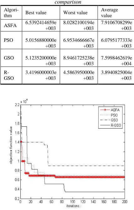
the unit is the minute. Optimized result comparison as Table 2, curves of the objective function value as Figure 1.

Table 2: Whenα =0.2,β =0.8, optimized result

comparison

Algori-

thm Best value Worst value

Average value ASFA 6.5392414659e

+003

8.0282100194e +003

7.9106708299e +003 PSO 5.0156880000e

+003

6.9534666667e +003

6.0795177333e +003 GSO 5.1235200000e

+003

8.9461725238e +003

7.5998462619e +004

R-GSO

3.4196000003e +003

4.5863950000e +003

3.8940825004e +003

[image:4.612.87.304.465.709.2]

In case 2, let

α

=

0.5,

β

=

0.5

, the operation

result is

min( (

F

∆

t

_k

))

=3893.40 ，

(2, 4,3,3, 2)

t

∆ =

the unit is the minute. Optimized result comparison as Table 3, the curves of the objective function value as Figure 2.

Table 3: α =0.5,β =0.5, Optimized Result Comparison

Algori-

thm Best value Worst value

Average value

ASFA 4.1531628190e +003

5.3329199363e +003

4.7430413776e +003

PSO 4.3350000000e +003

6.4919377976e +003

5.4134688988e +003

GSO 5.1012500000e +003

9.9330857142e +003

7.5171678571e +003

R-GSO

3.8929999999e +003

4.3030500000e +003

[image:5.612.84.524.74.545.2]

3.9880250000e +003

Figure 2: The Curves Of Objective Function Value

( α =0.5,β =0.5)

In case 3, when

α

=

0.8,

β

=

0.2

the operation

[image:5.612.309.521.97.483.2]

result is

min( (

F

∆

t

_k

))

=4946,

∆ =

t

(3, 2,5,1,14)

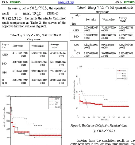
the unit is the minute. Optimized result comparison as Table 4, curves of the objective function value as Figure 3.

Table 4: Whenα =0.2,β =0.8 optimized result comparison

Algo ri

-thm

Best value Worst value Average value

ASFA

6.0764312047 e+003

7.2334575519 e+003

6.6549443783 e+003

PSO 6.3720819999 e+003

8.8179683333 e+003

7.5950251666 e+003

GSO 8.1924999999 e+003

9.9124562857 e+003

8.5524781428 e+003 R-

GS O

4.9459999999 e+003

5.0541999999 e+003

4.9824443809 e+003

Figure 3. The Curves Of Objective Function Value

(α =0.8,β=0.2)

Looking from the simulation result, in the early peak and in the late peak time interval, the computed result departure frequency is also high, tallies with the daily life situation. The weight value

β

α

,

has certain influence to the experimental result, but no matter in situation 1, 2 or 3 R-GSO all can make the good progress. In practical life application, the weight value

α β

,

, is decided with policy-maker's tendency direction.

5. CONCLUSIONS

[image:5.612.91.295.266.556.2]

R-GSO has obtained the good result in the convergence rate and the computational accuracy aspect. Calculated that machine the simulation experiment showed that this article proposed the algorithm can the effective application in the urban public transportation dispatching system, to manage solves public transit vehicles dispatching problem with the policy-maker to have the reference value.

ACKNOWLEDGEMENTS

This work is supported by National Science Foundation of China under Grant No. 61165015. Key Project of Guangxi Science Foundation under Grant No. 2012GXNSFDA053028, Key Project of Guangxi High School Science Foundation under Grant No. 20121ZD008.

REFRENCES:

[1] Zhang Feizhou. Intelligent dispatch for public traffic vehicles and its related technologies. Beijing: BeiHang University. 2000.

[2] Bo Lijun, Yao Weipeng, Wang Yanhui. The optimum Mathematical model on the bus dispatch.Journal of Engineering Mathematics. Vol.19, 2002, pp.67-74,.

[3] Ren Chuanxing, Xun Yijun, Yin Changchang. Research of bus dispatching based on genetic taboo search algorithm. Journal of Shandong

University of Science, Vol.27,2008, pp.53-56.

[4] Yan Feng, Guang Xiaoping. Model and algorithm analysis based on the two-tiered programming on bus scheduling. Journal of

Lanzhou Jiaotong University, Vol.27, 2008,

pp.75-79.

[5] Armin Fugenshuh. Solving a school bus scheduling problem with integer programming European Journal of Operational Research, Vol.193, 2009. pp.867-884.

[6] Krishnanand K. N. D. Ghose D. Glowworm swarm optimization: a new method for optimizing multi-modal functions.

Computational Intelligence Studies, 2009,Vol.

1, pp.93-119.

[7] Krishnanand K. N. Glowworm swarm optimization: a multimodal function optimization paradigm with applications to multiple signal source localization tasks. Indian: Department of Aerospace Engineering, Indian Institute of Science, 2007. [8] Krishnanand K. N. and Goose D.Theoretical foundations for rendezvous of glowworm-inspired agent swarms at multiple locations.

Robotics and Autonomous Systems, Vol.56,

2008, pp.549-569.

[9] Krishnanand K. N. and Ghose D. A glowworm swarm optimization based multi-robot system for signal source localization. Design and Control of Intelligent Robotic

Systems, pp.53-74,2009.

[10] Krishnanand K. N. and Goose D. Chasing multiple mobile signal sources: a glowworm swarm optimization approach. In Third Indian. International Conference on Artificial Intelligence, Indian, pp.54-58,2007.

[11]Fu Ali, Lei Siouan. Intelligent dispatching of public transit vehicles using particle swarm optimization algorithm. Computer

Engineering and Applications, Vol. 44,2008,

pp.239-241.

[12] Xiaolei Li, Jixian Qian. Artificial fish-swarm algorithm: Bottom-up optimization model. Trans Annual Meeting of Chinese Process

Systems Engineering Society.pp. 76-82,2001.

[13] Xiaolei Li, Z hijiang Shao, Jixian Qian. An optimizing method based on autonomous animats: fish-swarm algorithm, Systems

Engineering-Theory & Practice. Vol.22, 2002,

pp.32-38.

[14] Yongquan Zhou, Guo Zhou, Junli Zhang. A Hybrid Glowworm Swarm Optimization Algorithm for Constrained Engineering Design Problems .Applied Mathematics &

Information Sciences, Vol.7, No.1, 2013,

pp.379-388.