Visual attention using 2D & 3D displays

(1)

Visual Attention Using 2D & 3D Displays

by

Zbigniew Zdziarski, BA, BCompSc (Hons)

Dissertation

Presented to the

University of Dublin, Trinity College

in fulfillment

of the requirements

for the Degree of

Doctor of Philosophy

University of Dublin, Trinity College

(2)

Declaration

I, the undersigned, declare that this thesis has not been submitted as an exercise

for a degree at this or any other university and it is entirely my own work.

Zbigniew Zdziarski

(3)

Permission to Lend and/or Copy

I, the undersigned, agree to deposit this thesis in the University’s open access

insti-tutional repository or allow the library to do so on my behalf, subject to Irish Copyright

Legislation and Trinity College Library conditions of use and acknowledgement.

Zbigniew Zdziarski

(4)

Acknowledgments

Firstly I would like to thank Dr Rozenn Dahyot without whom I would never have

submitted this thesis. I was very lucky to have her as a supervisor and will undoubtedly

be recommending her to anyone wishing to do any research in computer vision.

Secondly I would like to thank everyone in the GV2 group for the laughs and good

times. I would especially like to thank Dr Claudia Arellano next to whom I sat in the

lab for over three years. We went through thick and thin together!

Next I would like to thank Kieran O’Reilly, frontman of the band White McKenzie

that I was fortunate enough to join on my arrival to Ireland. Kieran’s always been

there for me - a true mate. I will never forget you and hope that our friendship will

continue to develop even if greater distances will separate us.

Lastly I would like to thank all my other friends that made living away from

Aus-tralia (the place I will always call home) that little bit more bearable. People like Ryan

Connolly, Maria Salisbury, Br Conor McDonough, Br Michael O Dubhghaill, and Dr

Alvaro Paul deserve a special mention here. Cheers, guys.

Zbigniew Zdziarski

University of Dublin, Trinity College

(5)

Abstract

In the past three decades, robotists and computer vision scientists, inspired by

psy-chological and neurophysiological studies, have developed many computational models

of attentions (CMAs) that mimic the behaviour of the human visual system in

or-der to predict where humans will focus their attention. Most of CMA research has

been focussing on the visual perception of images and videos displayed on 2D screens.

There has recently, however, been a surge in devices that can display media in 3D and

CMAs in this domain are becoming increasingly important. Research in this context

is minimal, however. This thesis attempts to alleviate this problem. We explore the

Graph-Based Visual Saliency algorithm [68] and extend it into 3D by developing a new

depth incorporation method. We also propose a new online eye tracker calibration

procedure that is more accurate and faster than standard processes and is also able

to give confidence values associated with each eye position reading. Eye tracking data

is used to evaluate CMAs. We use our novel eye tracking method to create a 2D/3D

video eye tracking dataset obtained from 50 people. A statistical analysis is performed

to locate where perception differs in 2D and 3D in videos. Taking advantage of the

uncertainties associated with our eye tracking data, we also propose a novel Gaussian

(6)

List of Tables

2.1 VSAs presented in this section in their respective classes. * indicates a spatio-temporal algorithm. . . 21 2.2 Free-viewing eye tracking datasets on images available in the public

do-main for CMA evaluation and comparison. * indicates that images were displayed in 3D. . . 26 2.3 Free-viewing eye tracking datasets on videos available in the public

do-main for CMA evaluation and comparison. Dataset size is measured in number of video clips. . . 26

3.1 Percentage of training features correctly and incorrectly classified by the SVM. . . 35

4.1 Performances of 2D VSAs. Higher PLCC and lower KLD values indicate better performances. . . 49 4.2 Performances of 3D-VSAs. Higher PLCC and lower KLD values indicate

better performance. . . 52 4.3 Results for each image for GBVS, GBVS-Chamaret and GBVS-Our

method. Higher PLCC and lower KLD values indicate a better perfor-mance. # indicates that it is significantly different from the 2D model (paired t-test, p<0.1). . . 55

5.1 Estimated parameters for the spatio-temporal exponential variogram (cf. Fig. 5.2). . . 68

(10)

B.1 Eye tracking statistics from the left eye summarising 2D and 3D eye movements from the videos in group 1 (strong 3D). Euclidean distance is in pixels. . . 98 B.2 Eye tracking statistics from the left eye summarising 2D and 3D eye

movements from the videos in group 2 (little or no camera movement). Euclidean distance is in pixels. . . 99 B.3 Eye tracking statistics from the left eye summarising 2D and 3D eye

(11)

List of Figures

1.1 Foveated imaging example of a woman doing sign language. Image on right has its resolution adapted around the woman’s hand and face (taken from [175]). . . 2 1.2 An example of a heat map of a search results page. The hotter the

colour, the more attention was devoted to that area of the image for a given time period. Heat maps such as these can typically change as different time periods are analysed for users’ attention (image taken from [30]). . . 4 1.3 The original Buswell eye tracker and the well-known head-mounted

“Eye-link II” (SR Research Ltd, v. 2.0) eye tracker. . . 5

2.1 Architecture of the Koch and Ullman’s model (adapted from [169]) . . 11 2.2 Activation and normalisation example on two feature channels - intensity

and orientation. N(.) is a normalisation operator (adapted from [78]). . 12 2.3 The Koch and Ullman model (in red) with a motion channel attached

as explored by Itti in [76]. . . 14 2.4 Examples of classic synthetic patterns used in the comparison of VSAs

by Borji et al. [21]. . . 22 2.5 The motion cycle of an object in the spatio-temporal domain according

to work performed by Bulbul et al. [28]. . . 24 2.6 (a) Example image; (b) Fixation density map (ground truth); (c) Saliency

(12)

2.7 Fixation heat maps for all images from the: (a) Bruce dataset; (b) Kootstra dataset; and (c) Judd dataset. White rings depict 10% increase in distance from centre of the image (adapted from [21]) . . . 31

3.1 Flowchart of the training and testing phases of the experiment . . . 37 3.2 (a): proportion of correct classification for the horses dataset pp (solid

blue line) and 1−pn (green dashdot line) w.r.t. T; (b) proportion of

correct classification for the flowers datasetpp(solid blue line) and 1−pn

(green dashdot line) w.r.t. T; (c) proportion of correct classification for the faces dataset pp (solid blue line) and 1 −pn (green dashdot line)

w.r.t. T; (d) total no. of feature points np for horses (solid blue line),

flowers (green dashdot line) and faces (dotted red line) and nn (aqua

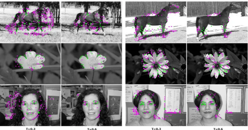
dashed line). . . 39 3.3 Example results for T = 0.3 and 0.6. From top to bottom: horses,

flowers and faces. Green dots indicate feature points classified in the image class (C), purple dots indicate feature points classified outside of it (C). . . .¯ 40 3.4 (a) Memory usage for positive images w.r.t.Tfor horses (solid blue line),

flowers (green dashdot line) and faces (red dotted line); (b) Classification computation time for positive images w.r.t.Tfor horses (solid blue line), flowers (green dashdot line) and faces (red dotted line). . . 41

4.1 Two depth incorporating strategies: (a) the depth-weighting model; (b) the depth-saliency model [172]. . . 46 4.2 Saliency maps with VSAs. (a) Original image #1 [173], (b)

Correspond-ing fixation density map, (c)-(f) Saliency predictions from the four 2D VSAs: Itti, Hou, Bruce and GBVS, (g)-(i) Saliency predictions from the three 3D VSAs: 3D GBVS (Wang), 3D GBVS (Chamaret) and 3D GBVS (Our method) . . . 50 4.3 Saliency maps with VSAs. (a) Original image #2 [173], (b)

(13)

4.4 Saliency maps with VSAs. (a) Original image #11 [173], (b) Corre-sponding fixation density map, (c)-(f) Saliency predictions from the four 2D VSAs: Itti, Hou, Bruce and GBVS, (g)-(i) Saliency predictions from the three 3D VSAs: 3D GBVS (Wang), 3D GBVS (Chamaret) and 3D

GBVS (Our method) . . . 53

4.5 Saliency maps with VSAs. (a) Original image #18 [173], (b) Corre-sponding fixation density map, (c)-(f) Saliency predictions from the four 2D VSAs: Itti, Hou, Bruce and GBVS, (g)-(i) Saliency predictions from the three 3D VSAs: 3D GBVS (Wang), 3D GBVS (Chamaret) and 3D GBVS (Our method) . . . 54

5.1 Three types of eye tracking devices . . . 58

5.2 Exponential variogram model. . . 63

5.3 A baby wearing the WearCam from [132]. . . 65

5.4 Example empirical and fitted variogram on real data from a particpant. 69 5.5 The 13 calibration points (red) and 3 test points (blue) used in the second stage of the experiment. The red-blue point was used as a cali-bration and test point. . . 70

5.6 Average degradation of accuracy of the eye tracker over the 22 experi-ments. Standard deviation shown as error bars. . . 71

5.7 Average error for each showing of the three test points with standard deviations obtained using the standard calibration method (red) and our kriging method (blue) over the 22 experiments. . . 72

5.8 Example image representing ∆x(x, y, t= 143) interpolated on the entire screen. . . 73

5.9 (a) ∆x for one pixel (a calibration point) for one person; (b) ∆y for the same person and point; (c) ∆x for one pixel (a calibration point) for another person; (d) ∆y for the same person and point; . . . 74

(14)

B.1 (a) Frame 55 from video #1; (b) optical flow for this and next frame; (c) disparity map; (d) & (f) eye position density maps in 2D and 3D; (e) & (g) corresponding single Gaussian representations. The difference between the Gaussians is significant. . . 100 B.2 (a) Frame 59 from video #1; (b) optical flow for this and next frame;

(c) disparity map; (d) & (e) eye position density maps in 2D and 3D. . 101 B.3 (a) Frame 186 from video #1; (b) optical flow calculation for this frame

and the next; (c) disparity map for this frame; (d) & (e) eye position density maps in 2D and 3D for this frame. . . 102 B.4 (a) Frame 242 from video #1; (b) optical flow calculation for this frame

and the next; (c) disparity map for this frame; (d) & (e) eye position density maps in 2D and 3D for this frame. . . 103 B.5 (a) Frame 416 from video #1; (b) optical flow calculation for this and

next frame; (c) disparity map for this frame; (d) & (e) eye position density maps in 2D and 3D for this frame. . . 104 B.6 (a) Frame 184 from video #2; (b) disparity map; (c) & (d) eye position

density maps in 2D and 3D. (e) Frame 55 from video #2; (b) disparity map; (g) & (h) eye position density maps in 2D and 3D. . . 105 B.7 (a) Frame 234 from video #2; (b) disparity map; (c)&(d) eye position

density maps in 2D and 3D. (e) Frame 280 from video #2; (b) disparity map; (g)&(h) eye position density maps in 2D and 3D. . . 106 B.8 (a) Frame 165 from video #3; (b) disparity map; (c)&(d) eye position

density maps in 2D and 3D. (e) Frame 335 from video #3; (b) disparity map; (g)&(h) eye position density maps in 2D and 3D. . . 107 B.9 (a) Frame 150 from video #4; (b) disparity map; (c)&(d) eye position

density maps in 2D and 3D. (e) Frame 193 from video #4; (b) disparity map; (g)&(h) eye position density maps in 2D and 3D. . . 108 B.10 (a) Frame 150 from video #5; (b) disparity map with new drop

(15)

B.11 (a) Frame 635 from video #5; (b) disparity map for this frame with new drop highlighted; (c) & (d) eye position density maps in 2D and 3D for this frame. . . 110 B.12 (a) Frame 98 from video #7; (b) disparity map; (c)&(d) eye position

density maps in 2D and 3D. (e) Frame 863 from video #7; (b) disparity map; (g)&(h) eye position density maps in 2D and 3D. . . 111 B.13 (a) Frame 170 from video #8; (b) disparity map; (c) & (d) eye position

density maps in 2D and 3D. (e) Frame 285 from video #8; (b) disparity map; (g) & (h) eye position density maps in 2D and 3D. A different disparity map extraction algorithm is used in (f) because the one from Sun et al. [162] would not detect the boat. . . 112 B.14 (a) Frame 450 from video #8; (b) disparity map for this frame; (c) &

(16)

Chapter 1 Introduction

We never see and analyse an entire scene completely in one go [182]. Every second approximately 108_-109 _{bits of visual stimuli enters our eyes [76, 95, 20]. This is too}

much information for the human visual system to handle in real-time so it optimises the analysis of scenes by picking out important information in regions. When given a scene, we move our gaze from one important region to another - and it is during this time that the brain builds its representation.

This optimising action of ours, calledselective attention, is the subject of research in visual attention (VA). Inspired by psychological and neurophysiological studies, robo-tists and computer vision scienrobo-tists have attempted to build systems that mimic the behaviour of the human visual system in order to predict where humans will focus their attention. As a consequence, in the past three decades numerous computational models of attention (CMAs) that attempt to locate salient regions in images and videos have been proposed.

1.1 Applications of Visual Saliency

There is a clear need for the study of VA and CMAs. Indeed, CMAs have proven useful in a number of applications. These would include:

(17)

Figure 1.1: Foveated imaging example of a woman doing sign language. Image on right has its resolution adapted around the woman’s hand and face (taken from [175]).

searching over these descriptions when a user queries for an image/video. Visual saliency can be used here to describe only the most important sections or regions of a media file, hence minimising the search space and retrieval time.

(18)

• Image and video quality assessment. Image and video quality can decrease as a result of compression. It is often useful to calculate the quality of media to see, for example, if the compression level is too large or to calculate the efficiency of a compression algorithm with respect to visible change. Visual saliency has been used in this task. Ma and Zhang [112], You et al. [185] and Feng et al. [51] assessed such media quality by giving more weight to quality measurements in salient regions. The justification for this is that it should be more important to measure the quality of salient regions rather than regions that a user will ignore.

• Control of vehicles and robots, navigation, and surveillance. Quickly calculating the state of a situation or analysing an environment by sifting out irrelevant data is significant in automating vehicular [149] and robotic control [53], [2], [155] and in tasks such as wilderness search and rescue [148]. CMAs can also be used in surveillance where important regions can be a factor in determining the position/viewpoint of a camera [8].

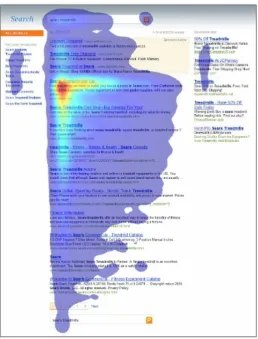
• Automatic evaluation of advertisements, web pages, interface designs, etc. [77], [29], [113]. Eye tracking is frequently utilised by advertising, web page and magazine design companies to assess the effectiveness of an advertisement, interface design, etc. An example of a heat map obtained from eye tracking of a search results page is shown in Figure 1.2. Eye tracking is, however, un-comfortable for the user and expensive, and automating this task would be very financially beneficial to these companies and others working with visual attention [43] [42].

1.2 Eye Tracking and Visual Attention

(19)

[image:19.595.191.450.127.467.2]

Figure 1.2: An example of a heat map of a search results page. The hotter the colour, the more attention was devoted to that area of the image for a given time period. Heat maps such as these can typically change as different time periods are analysed for users’ attention (image taken from [30]).

what is calledcovert attention (discussed further in Section 2.1.1). Regardless of these findings, the eye-mind hypothesis is still a useful tool for measuring the correlation between visual attention and eye positions. Indeed, most research on VA uses this hypothesis [87].

(20)

(a) The Buswell Eye Tracker [31] (b) The Eyelink II Eye Tracker1

Figure 1.3: The original Buswell eye tracker and the well-known head-mounted “Eye-link II” (SR Research Ltd, v. 2.0) eye tracker.

they accounted for approximately 100 pixels of error on a 1920 x 1200 LCD monitor when attempting to determine which object was being viewed [125]. Moreover, top-of-the-range eye trackers are very expensive - prices range from e4000-e30,000. It is necessary, therefore, to attempt to improve the accuracy of eye trackers - at least to avoid the infeasible (for most) notion of constantly upgrading eye trackers with newer, more accurate models when they become available.

1.3 Visual Attention in 2D & 3D

Most of VA research has been focussing on the visual perception of images and videos displayed on 2D screens. More recently, however, it has been shown that humans look differently at images displayed in 3D compared to 2D [172]. For example Jansen et al. [82] found that for images shown in 3D, people fixate more, have shorter and faster saccades (the movement of the eyes between fixations) and tend to explore more with their eyes.

Due to the differences in viewing behaviour CMAs, to be as accurate as possible,

1_{Image adapted from}

(21)

need to be specifically tuned or rebuilt for 3D media. Since 3D media is becoming ubiquitous (e.g. 3D films in cinemas or at home, 3D games, 3D hand-held devices such as mobile phones and the Nintedo 3DS) this is becoming an increasingly important area of research. Ultimately, all the applications listed above will need to be ported to the 3D domain.

Another problem is that the research that has been performed to compare 2D and 3D VA on videos is minimal. For example, no ground-truth eye tracking dataset exists for 3D videos. Without such a dataset, it is impossible to accurately verify the preciseness of 3D CMAs.

This thesis specifically focusses on 3D VA and CMAs and presents work that fur-thers this scientific field and helps with the problems mentioned above. It also presents a method to improve current state-of-the-art eye tracking measurement.

1.4 Contributions of this Ph.D.

The contributions of this thesis can be summarised as follows:

• In Chapter 3 we show that CMAs can be used to optimise content-based image retrieval and other such systems. By describing images containing only one dom-inant object using feature points solely collected from salient regions (as opposed to feature points obtained from the entire image), we show that an improvement in classification results can be obtained. We use the Graph-Based Visual Saliency Algorithm (described in detail in Section 4.1.1) to show that this algorithm can be applied to real applications. This algorithm is then used on 3D images in the following chapter.

• In Chapter 4 we extend the 2D Graph-Based Visual Saliency Algorithm into 3D by developing a new depth incorporation method. This new 3D CMA outper-forms all other state-of-the-art 3D algorithms on 3D media.

(22)

values associated with each eye position reading - something that current eye tracking procedures are unable to do.

• To better understand the differences in 2D and 3D viewing behaviour in videos we ran a full-scale eye tracking experiment with 50 participants who looked at professionally made videos. This experiment was done using our eyetracking procedure presented in Chapter 5. Chapter 6 presents this experiment and an analysis of the difference in viewing behaviour between the 2D and 3D videos. In this chapter we also present a more scientific way of presenting eye tracking heat maps. We hope that the analysis presented here will enable any future work in 3D VA to be improved. The resulting eye tracking dataset from this chapter will also be made available in the near future to the public. As was mentioned above, no such eye tracking datasets currently exist.

1.5 Publications

The work presented in this thesis has been published in the papers listed below:

• Z. Zdziarski and R. Dahyot. “Feature selection using visual saliency for content-based image retrieval”. IET Irish Signals and Systems Conference, pages 1-6, 2012.

• Z. Zdziarski and R. Dahyot. “On creating a 2D & 3D visual saliency dataset”. Proc. of the ACM Symposium on Applied Perception, page 132, 2013.

(23)

Chapter 2 Background

This background review is based on three seminal Ph.D.’s on the topic (Bruce 2008 [23], Gao 2008 [55], and Judd 2011 [87]), a recent state-of-the-art review published in 2013 by Borji and Itti [20] and is supplemented by new material published since.

Before any work, however, on visual attention (VA) and computational models of attention (CMAs) is presented, a definition ofattentionneeds to be given. Perhaps the best such definition was provided by William James in 1890 [81]: “[Attention] is the taking possession by the mind, in clear and vivid form, of one out of what seems several simultaneously possible objects or trains of thought. Focalization, concentration, of consciousness are of its essence. It implies withdrawal from some things in order to deal effectively with others”. This thesis, of course, focusses on visual attention, which deals with attention on visual stimuli.

2.1 Attention Mechanisms

(24)

2.1.1 Covert Versus Overt Attention

Attention can be distinguished by being either covert or overt. The overt attention mechanism involves specifically moving one’s fovea to a region of interest and paying attention to it [59, 154]. For example, if you are listening and looking at someone talking to you, you are engaging the overt mechanism of attention. Covert attention does not explicitly involve movement of the eyes and head [59, 154]. An example of covert attention is concentrating on an object in the corner of one’s eye. Another example is one of driving: when driving a driver focusses on the road while simultaneously keeping track of signs and traffic lights.

Covert and overt attention normally operate together [52]. It is widely believed that covert attention is used to locate interesting regions for overt attention to fixate on [20, 142]. This process was described in Chapter 1. Nonetheless, it is still possible to pay attention to things not directly encompassed by the fovea [87]. This is an ongoing piece of research and currently the standard course of action in CMA research is to not deal explicitly with covert attention. This thesis will follow suit.

2.1.2 Bottom-Up and Top-Down Attention

(25)

objects and from these possibilities locate the desired toy - we have prior (top-down) information so we know which salient features need to be given more weight. CMAs are distinguished by whether they rely on bottom-up influences, top-down influences or a combination of both.

Top-down saliency is a difficult problem in itself and many questions remain unan-swered. E.g. are bottom-up and top-down calculations performed independently or does one influence the other? If the latter, how is this performed? How do you predict top-down influences? Because of such questions, and since bottom-up CMAs are sim-pler and easier to understand and implement many applications choose to remain with bottom-up CMAs. In fact, bottom-up CMAs are considered to be ‘general purpose’ attention algorithms and most research in VA is conducted on bottom-up models [20]. This thesis also focusses on bottom-up saliency.

2.2 Bottom-Up Visual Saliency Algorithms

When discussing bottom-up CMAs we limit ourselves to models that compute saliency maps for videos or images. Saliency can be understood as something that characterises parts of a scene that stand out from its surroundings. Parts of a scene can be regions or objects, for example. A saliency map, therefore, is a scalar, two-dimensional map that indicates the saliency value (conspicuity) for every pixel in an image [87]. Models that do not compute saliency maps are outside of the scope of this thesis and computer vision in general [20]. The termvisual saliency refers to visual attention that focusses on up processes [21]. Visual saliency algorithms (VSAs) are, therefore, bottom-up CMAs.

2.2.1 Origins

(26)

[image:26.595.215.426.129.378.2]

Figure 2.1: Architecture of the Koch and Ullman’s model (adapted from [169])

proposed a model of this theory in 1985. Saliency in the Koch and Ullman model is first calculated by extracting the visual cues of colour, orientation and intensity from an image. An activation map (an initial saliency map) is then calculated in parallel for each of these channels. Next, the activation maps are combined into a master saliency map. Finally, a ranking of salient regions is computed through the use of a Winner-Takes-All (WTA) network. The architecture of the Koch and Ullman model is shown in Figure 2.1.

The process of obtaining a master saliency map (without the WTA step) can be summarised in three stages as suggested by Harel et al. in [68]:

1. extraction

2. activation

3. normalisation/combination

(27)

Figure 2.2: Activation and normalisation example on two feature channels - intensity and orientation. N(.) is a normalisation operator (adapted from [78]).

[124]) shows the salient areas of an image for a given feature channel (e.g. intensity, colour, etc.). So, for example, in the colour feature channel a yellow blob will be given higher saliency values if this blob is located on a completely black background. Or a vertical bar will be given a high saliency value in the orientation channel if the only other bars in the image are horizontal. Difference of Gaussian (DoG) is a common way of calculating saliency for each feature channel. This approach involves constructing a Gaussian pyramid for each channel and comparing the differences between scales.

The normalisation/combination stage involves the normalisation of activation maps and then amalgamation of them into one master saliency map. Normalisation is nec-essary since the feature cues are not all in the same range. Normalisation also takes into consideration relative differences in an activation map.

The first step shown in Figure 2.2 demonstrates the creation of an activation map for the intensity and orientation channels of an example image. This activation map is then normalised (second step in the figure) to be ready for global amalgamation into a master saliency map.

(28)

Since the Koch and Ullman model many more models have been proposed and implemented. The most important of these will be presented in the next section.

2.2.2 Other Important VSAs

In their review, Borji and Itti [20] divided VSAs into eight classes: cognitive, bayesian, decision theoretic, information theoretic, graphical, spectral analysis, pattern classifi-cation, and others. This thesis will follow suit. The VSAs described here have been either influential/pioneering in the study of visual saliency and/or performed well in the exhaustive comparison of 35 state-of-the-art VSAs that was made by Borji, Sihite and Itti [21] in 2013.

Cognitive models

Cognitive models are strongly based on psychological and neurophysiological findings such as, for example, Treisman and Gelade’s [165] “Feature Integration Theory” de-scribed above. Itti’s [78] implementation of the Koch and Ullman model is, therefore, the first obvious VSA that belongs in this section. His implementation subsamples an image into a Gaussian pyramid [63] of nine levels. Each pyramid level is then decom-posed into channels for Red (R - calculated asr−(g+b)/2), Green (G=g−(r+b)/2), Blue (B =b−(r+g)/2), Yellow (Y = (r+g)/2− |r−g|/2−b), Intensity (the grey-scale version of the image), and local Orientations (O - calculated using the Gabor filter at angles 0, 45, 90, and 135 degrees). From these, feature mapsfl are calculated

by centre-surround (cs) operations. csoperations are defined as the difference between fine and coarse scales. For example, if the centre is a pixel at scale c ∈ {2,3,4}, the surround is the corresponding pixel at scale s =c+d, where d∈ {3,4}. After the cs

operations, the feature maps are then normalised:

fl =N(

4

X

c=2

c+4

X

s=c+3

fl,c,s),∀l ∈LI ∪LC ∪LO (2.1)

where

LI ={I}, LC ={RG, BY}, LO ={0◦,45◦,90◦,135◦} (2.2)

(29)

In total, the cs operation is performed on 42 maps (6 for intensity, 12 for colour, and 24 for orientation). The calculated feature maps are finally linearly summed and normalised once more into a master saliency map. Variations and extensions of this implementation have been proposed by Frintrop [52], Walther in the Saliency Toolbox [170], and Walther et al. [171].

[image:29.595.183.461.402.667.2]

Itti in [76] used the concept of adding an additional channel for motion to the Koch and Ullman model for the video domain. This addition is depicted in Figure 2.3 with the red boundary showing the standard Koch and Ullman model. Along with standard colour, intensity and orientation information, Itti added two temporal feature channels: temporal flicker (flickering of light intensity) and four oriented motion energies: up, down, left, and right. Just like in the Koch and Ullman model, all these feature channels were normalised and then merged into a single saliency map. Interestingly, Itti applied this model to foveation. He reports a 50% average increase in video compression rate performance for MPEG-1 and MPEG-4 video clips.

(30)

Since the Koch and Ullman model was proposed, research and understanding of the human visual system (HVS) has advanced. Le Meur et al. [100] proposed a VSA that modelled the HVS in a more complex way. Contrast sensitivity functions, visual masking and perceptual grouping are some of the additional functions they implemented. This algorithm was shown to outperform Itti’s [78]. Le Meur et al. [101] later extended their model to the spatio-temporal domain by proposing a fusing algorithm for achromatic, chromatic and temporal information.

Marat et al. [120] proposed a spatio-temporal VSA that was inspired by the first steps of the HVS. Modelling the output of the retina, two signals are extracted from a video stream: parvocellular and magnocellular. Static and dynamic information (signal orientation, spatial frequencies and optical flow calculated using spatial Gabor-like filters [27]) is then extracted from these streams from which two saliency maps are calculated. These are finally fused into a spatio-temporal map. Marat et al. showed that they were able to accurately predict the eye movements of subjects for the first few frames of each short clip they analysed.

Bayesian models

In bayesian models, prior knowledge about the scene (e.g. scene context or gist) and sensory information (e.g. target features) are combined probabilistically in Bayes’ rule to detect salient regions or objects of interest. Only one notable bottom-up algorithm from this class has been proposed.

Itti and Baldi [79] introduced a Bayesian definition of surprise as being something that changes the beliefs of an observer. Prior beliefs of an observer are captured and new data being observed is said to be surprising if the posterior resulting from new observations significantly differs (according to the KL divergence measure) from the prior. For images, prior information is taken as neighbouring locations. In the time domain, prior information at one point is captured from previous observations.

Decision theoretic models

(31)

CMAs should be optimised with respect to the end task. Most models in this class are top-down in nature but some have been implemented to remain bottom-up while maintaining a decision theoretic framework.

Gao and Vasconcelos [56] define a decision theoretic formulation of saliency of visual features at a given location as the power (expected classification accuracy) of those features to discriminate (distinguish) between them and a null hypothesis. In bottom-up visual saliency, the null hypothesis for Gao and Vasconcelos is the neighbourhood (surroundings) of the given location. Optimality is defined in the minimum probability of error sense.

The binary classification problem (i.e. discriminating between stimuli of interest against the null hypothesis) in decision theoretic models is extended to the temporal domain by Mahadevan and Vasconcelos [115, 116]. They included motion features in a bottom-up saliency mode. Similarly to Gao and Vasconcelos [56], the neighbourhood is defined as the null hypothesis. Their spatio-temporal model was shown to robustly identify salient moving objects for complex backgrounds by using dynamic texture models as a substitute for optical flow (that can be used for more static clips).

Information theoretic models

Information theoretic models aim to detect regions that maximise the information sampled from an environment. That is, they aim to detect the most informative regions while discarding the rest.

Bruce and Tsotsos [24] developed the well-known AIM model (Attention based on Information Maximisation) that uses Shannon’s self-information measure. Saliency of a region is calculated as the information it conveys relative to its surroundings. This is calculated as I(X) = −log(p(X)), where X is a visual feature and p(X) is the probability of observing X based on its surround. To calculate p(X), independent component analysis (ICA) is used to reduce the dimensionality of the problem. The bases for ICA are learned by sampling from a large number of random patches from natural images (since a single image will not have enough data for this). The final saliency value for a given image region is the product of the probabilities of observing this region for each ICA basis coefficient.

(32)

he calculates on a global and local level. Global contrast is measured by analysing histograms and local contrast by a centre-surround operation similar to that of Itti et al. [78]. Rarity is first calculated by computing the mean and variance of the neigh-bourhood and using other features such as size and orientation (e.g. smaller areas get higher saliency values). Finally, higher-level methods (e.g. Gestalt laws of grouping) are used to locate the salient regions.

Wang et al. [174] proposed a computational model to simulate human saccadic scanpaths on natural images. They integrated three factors to guide eye movements sequentially: 1) reference sensory responses (to provide a representatinon of the raw input signal); 2) fovea-periphery resolution discrepancy (to provide detailed informa-tion around a locainforma-tion and coarse details from the periphery); and 3) visual working memory (to prevent fixations from returning to previously fixated regions too early). For each eye movement, three multi-band filter response maps are calculated for the three factors. These filter response maps are then combined into multi-band residual filter response maps on which residual perceptual information (site entropy rate) is calculated at each location. Fixations are ordered by residual perceptual information scores.

Graphical models

Graphical models have a probabilistic graph model denoting the conditional indepen-dence between different variables. Graph-based approaches such as Hidden Markov Models, Dynamic Bayesian Networks and Conditional Random Fields can be employed in calculations.

(33)

Liu et al. [110] tackle the visual saliency problem for images with a single salient object. They propose new features to be used in their calculations such as multiscale contrast, center-surround histogram, and color spatial distribution. These are used to describe a salient object locally, regionally and globally. They use images from a large annotated dataset of 20,000+ images to train a conditional random field to effectively combine these features. Their model is extended to the spatio-temporal domain (Liu et al. [109]) by adding motion features (using SIFT flow [107]) to their calculations.

Spectral analysis models

Spectral analysis models perform their saliency calculations in the frequency domain as opposed to the spatial domain. These models are generally simple to explain and implement and can generate saliency maps in real-time.

Hou et al. [74] explored the properties of backgrounds by investigating the log spectrum of images to then extract the spectral residue. Finally, the spectral residue was transformed to the spatial domain to create a saliency map. This spectral residue technique has been used previously in, for example, sensory input to detect unexpected signals or anything that varies from the norm [12, 93].

The first step in Achanta et al.’s [4] model is to transform the colour image I to the CIELAB colour space. The saliency map is then calculated as:

S(x, y) =||Iµ−Iwhc|| (2.3) where x, y are pixel coordinates, Iµ is the arithmetic mean image feature vector, Iwhc is a Gaussian blurred (with a 5 x 5 separable binomial kernel) version of I and ||.|| is the euclidean distance. Achanta et al. is an example of a global contrast VSA meaning that it measures the saliency of a pixel by calculating its contrast to every other pixel in the image. These methods are good at detecting single salient objects on simple backgrounds but their performance deteriorates the more complex a scene becomes [184].

(34)

the image ratio being retained). A windowed Fourier transformF is then calculated:

f(u, v) =F[w(I(x, y))] (2.4)

where I(x,y) is the resized grey-scale image andwis a windowing function. A whitened (or normalised/flattened) spectral responsen is obtained by:

n(u, v) = f(u, v)/||f(u, v)|| (2.5)

This response is then transformed into the spatial domain (reverse Fourier transform), squared to further enhance the salient regions and convolved with a Gaussian low-pass filter:

S(x, y) =g(u, v)∗ ||F−1[n(u, v)]||2 _(2.6)

where g is a Gaussian filter. The model is further extended to the spatio-temporal domain by attempting to separate background motion from localised (salient) motion. Background motion is detected by utilising phase correlation [39] of two frames. The resulting motion vector for panning movement is used to shift the global motion of the two frames to extract the local motion.

Pattern classification models

In these models machine learning techniques are used to model visual attention. The techniques use pre-recorded eye fixations or manually labelled salient regions as training data.

Kienzle et al. [92] used eye tracking data to train a support vector machine (SVM) to model attention. Their aim was to find the functional relationship between image patches and their corresponding visual saliency. The SVM was trained on a non-linear mapping between these patches and their saliency scores (obtained from 200 grey-scale images that were viewed by 14 people). Positive values were given to patches that had been fixated on and negative values to randomly selected patches. Only the intensity channel was used.

(35)

gathered from eye tracking data obtained from 15 people who viewed 1,003 images.

Other models

Other models that do not conform to the above classes are described in this section. Goferman et al. [60] propose a more context-aware VSA. Four principles of human attention govern their salient region detection mechanism: low-level feature (colour, contrast, etc.) considerations, the suppressing of frequently occurring features on the global scale, the idea that salient patches tend to group together, and finally high-level feature considerations such as faces. Goferman et al. applied their VSA to image retargetting and summarisation.

Garcia-Diaz et al. [58] presented the Adaptive Whitening Saliency (AWS) model that is based on the adaptive whitening of colour and scale features. This is achieved through decorrelation and contrast normalisation in several steps in a hierarchical ap-proach. The first step is to transform an (r, g, b) image into a whitened (z1, z2, z3)

representation. This representation is acquired through decorrelation by employing principal component analysis over multi-scale low-level features. A bank of log-Gabor filters is used (for orientations of 0, 45, 90, and 135 degrees) to create feature maps over (z1, z2, z3). Seven scales are calculated for z1 and five each for z2 and z3. Each

feature map from the chromatic component is then whitened and contrast normalised in a hierarchical manner. The square of the vector norm in the resulting representation is the final saliency computation.

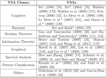
Table 2.1 shows the VSAs presented in this section accordingly classified into one of the eight VSA classes.

2.2.3 Summary of VSAs

(36)

VSA Classes VSAs

Cognitive

Itti (1998) [78], Itti* (2004) [76], Walther (2006) [170], Walther et al. (2002) [171], Frin-trop (2006) [52], Le Meur et al. (2006) [100], Le Meur et al.* (2007) [101], and Marat et al.* (2009) [120]

Bayesian Itti and Baldi* (2004) [79]

Decision Theoretic Gao and Vasconcelos (2009) [56] and Ma-hadevan and Vasconcelos* (2009) [115, 116]

Information Theoretic Bruce and Tsotsos (2009) [24], Mancas (2007) [118] and Wang et al. (2011) [174]

Graphical Harell et al. (2007) [68], Liu et al. (2007) [110], and Liu et al.* (2008) [109]

Spectral Analysis Hou and Zhang (2006) [74], Achanta et al. (2009) [4], and Bian and Zhang* (2009) [17]

Pattern Classification Kienzle et al.* (2009) [92] and Judd et al. (2009) [88]

[image:36.595.137.505.127.396.2]

Others Goferman et al. (2012) [60] and Garcia-Diaz et al. (2009) [58]

Table 2.1: VSAs presented in this section in their respective classes. * indicates a spatio-temporal algorithm.

report a number of findings. First, for synthetic images, models based on the feature integration theory performed well (e.g. Itti et al. [78] and Frintrop et al. [52]). The best results were obtained by Harel et al.’s GBVS algorithm [68]. Garcia-Diaz et al. [58] and Bian and Zhang [17] performed highly as well. Synthetic images were classic patterns that have been frequently used for psychophysical experiments and evaluation of attention models. These patterns contain only one item (target position) in each image that differs from all other (distractor) items. Example synthetic patterns used in the comparison experiments can be seen in Figure 2.4.

(37)

(a) Difference in colour (b) Assymetry in one item (c) Difference in orienta-tion

Figure 2.4: Examples of classic synthetic patterns used in the comparison of VSAs by Borji et al. [21].

is, on average, GBVS out-scores all other models when using the NSS and CC metric. Garcia-Diaz et al. [58] is the best performer for both datasets with the shuffled AUC metric. Bian et al. [17] performed second-best. In light of these results for videos, Borji, Sihite and Itti call for the best performing static models to be extended into the spatio-temproal domain to possibly improve their results even more. With respect to computation time, Hou et al. [74] and Bian and Zhang [17] are the two fastest VSAs (0.30 secs and 1.1 secs on average, respectively) implemented in Matlab. These provide an option for trade-off between accuracy and speed sometimes necessary for real-life applications.

2.2.4 Saliency and Motion

(38)

It was already mentioned in Section 2.2.2 that Itti in [76] used the simple concept of adding an additional channel for motion to the classic Koch and Ullman model (cf. Figure 2.3). Itti compared his motion saliency results against human behaviour (with an eye tracker) to show that “subjects preferentially fixated locations which the model also determined to be of high priority, in a highly significant manner”.

Williams and Draper published an interesting paper in which they concluded that “adding motion channels does not improve the performance of saliency-based selective attention” [180]. They used the same approach as Itti in [76] by adding a separate motion channel to the Koch and Ullman model. Their conclusion is surprising but a criticism of their report is that they used an overly simplistic motion analysis method - the Lucas-Kanade algorithm. This algorithm only looks at two adjacent frames for detecting potential salient regions. If the motion estimation algorithm is not accurate (i.e. not robust), then this may explain why it does not provide good information for saliency.

A complex solution was proposed by Jeong et al. in [83]. Their system is an amal-gamation of bottom-up and top-down saliency techniques that combine motion, sym-metry, as well as depth information. Motion information is analysed in the penultimate stage of saliency calculation: after standard low-level feature analysis and before in-corporating depth data. Their motion analysis uses the model proposed by Fukushima in [54] and is partly biologically based. Motion analysis is only conducted on salient regions as calculated in step 1 and the rotation, expansion, contraction, and planar characteristics of motion as well as temporal contrast changes (used to retrieve local and then later relative velocity) are then examined. Motion changes in each of these characteristics were given different weight values. Results from this were merged with depth information to produce a final saliency map.

(39)

[image:39.595.103.535.235.446.2]

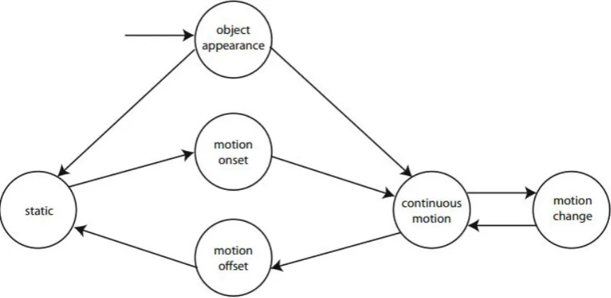
of return principle (if an object has already been viewed, its saliency value will be decreased). Each of these states have different saliency values, which were quantified by eye tracking experiments. Furthermore, a global saliency value is attributed to each object according to all relationships with other objects. Figure 2.5 depicts the motion cycle of an object, i.e. its 6 possible states and the relationships between them.

Figure 2.5: The motion cycle of an object in the spatio-temporal domain according to work performed by Bulbul et al. [28].

(40)

are consistent for a certain minimum amount of duration are deemed to be salient and flagged as belonging to the foreground. Their background subtraction technique was shown to significantly outperform many state-of-the-art approaches.

Also recently, Li et al. [104] proposed a saliency-based unsupervised video object ex-traction framework. First, to detect each moving part, motion saliency was calculated using dense optical flow forward and backward propagation. Then, shape informa-tion was learned through moinforma-tion cues for characterising each detected object. Next, standard saliency calculations (using colour and contrast information) were used to supplement the motion-induced shape information. Finally, conditional random fields were employed to combine the salient features to automatically detect objects. This technique was shown to deal well with unknown pose and scale variations of objects.

2.3 Eye Tracking Datasets

There are a number of eye tracking datasets available in the public domain for both images and videos. We limit ourselves here to presenting only those datasets that are predominantly used to evaluate and compare VSAs. Since we are dealing with only bottom-up saliency in this thesis, we also only present datasets in which participants were free-viewing (i.e. were not given a task to perform during the experiment). All participants in these datasets had normal or corrected-to-normal vision.

2.3.1 Image Datasets

Table 2.2 shows the datasets available in the public domain for images. Wang et al. [173] is the only dataset with 3D images.

2.3.2 Video Datasets

(41)

Study Subjects Dataset Size Resolution

Kienzie et al. [92] 14 200 1024 x 768

Einhauser et al. [44] 7 54 640 x 480

Bruce and Tsotsos [26] 20 120 681 x 511

Stark and Choi [158] 7 15 15 x 20cm

Judd et al. [88] 15 1003 Various

Cerf et al. [33] 7 250 1024 x 768

Peters et al. [141] 4 100 Various

Kootstra et al. [98] 31 99 1024 x 768

Tatler [164] 14 48 800 x 600

Engmann et al. [48] 8 90 1280 x 1024

Engelke et al. [47] 30 7 512 x 512

Le Meur et al. [100] 40 46 800 x 600

Rajachekar et al. [146] 29 101 1042 x 768

Wang et al. [173] 35 18* 1920 x 1080

Table 2.2: Free-viewing eye tracking datasets on images available in the public domain for CMA evaluation and comparison. * indicates that images were displayed in 3D.

Study Subjects Dataset Size Length Resolution

Mital et al. [128] 42 26 42mins 1280 x 960

Marat et al. [119] 15 324 68secs 720 x 576

Le Meur et al. [101] 17-27 7 98secs 800 x 600 Mathe and Sminchisescu [122] 4 3869 21hrs Various

Dorr et al. [41] 54 18 6mins 1280 x 720

Hadizadeh et al. [65] 15 12 105secs 352 x 288

Alers et al. [6] 12 25 8mins 1280 x 720

[image:41.595.162.478.127.343.2]

Li et al. [105] 14 50 8mins 1920 x 1080

Table 2.3: Free-viewing eye tracking datasets on videos available in the public domain for CMA evaluation and comparison. Dataset size is measured in number of video clips.

2.4 Evaluation Measures

(42)

There is no consensus as to which or how many of these methods should be used to assess a VSA. In practice one, sometimes two, methods are used and these are chosen at the VSA authors’ discretion [20]. To assess VSAs these metrics can be used on the publically available eye tracking datasets (for images and videos) described in the previous section.

2.4.1 Kullback-Leibler Divergence (KLD)

The KLD is usually used to measure the distance between two probability distributions. It is similarly used in the context of visual saliency where it calculates the dissimilar-ity between the saliency maps obtained from saliency algorithms with fixation densdissimilar-ity maps (maps created from eye tracking experiments). Fixation density maps are ob-tained by convolving a Gaussian filter across fixation locations of all observers [88]. These maps are treated as two probability density functions (PDFs), defined asH and

P respectively in the following equation:

KLD(H, P) =X

x

hxln

hx

px

(2.7)

wherehx and px denote the values of the normalised maps of H and P respectively at

pixel location x [100, 126]. The lower the KLD value obtained, the better the result (with a value of 0 denoting equality). This metric was used to assess a VSA, for example, in the studies of Wang et al. [173] and Itti and Baldi [79].

2.4.2 Pearson Linear Correlation Coefficient (PLCC)

The PLCC measures the linear correlation between the saliency and fixation density mapsH and P:

PLCC(H, P) = Cov (H, P)

σHσP

(2.8)

where Cov(H, P) is the covariance and σH and σP denote the standard deviations of

(43)

2.4.3 Area Under Curve (AUC)

The AUC metric is the area under the Receiver Operating Characteristic (ROC) curve [62] on the saliency and fixation density maps. Each map is processed by a binary classifier (a variable threshold) applied to every pixel. If a value in the saliency map is larger than a threshold it is said to be fixated on with the rest of the pixels said to be nonfixated [26, 33]. The same is done to the fixation density map and a comparison between fixated and nonfixated pixels is made between the two maps. The threshold of the binary classifier is varied and an ROC curve is drawn as the false positive rate versus the true positive rate. The area under this curve is said to indicate how well the saliency map aligns with the ground truth (with the value of 1 indicating a perfect alignment) [20, 126].

Figure 2.6 shows (a) an example image, (b) corresponding fixation density map, (c) saliency (prediction) map and then (d) & (e) the top 20% of the salient areas from the ground truth and saliency map with (f) the classification result and (g) the final ROC curve. In this example the AUC is approximated by a left Riemann sum (represented by the red rectangles).

The AUC metric was used, for example, by Harel et al. [68] and Bruce and Tsotos [26] to assess their VSAs.

2.4.4 Normalised Scanpath Saliency (NSS)

(44)

(a) Example image (b) Fixation density map (c) Saliency map

(d) Top 20% from fixation den-sity map

(e) Top 20% from saliency map (f) Combination

(g) AUC Graph

Figure 2.6: (a) Example image; (b) Fixation density map (ground truth); (c) Saliency map; (d) & (e) top 20% regions of the fixation and saliency maps respectively; (f) Classification results: red - true positives, green - false negatives, blue - false positives, other areas are true negatives; (g) ROC curve (adapted from [126]).

2.4.5 String Edit Metric

(45)

ob-server from region ‘a’ to ‘b’ then to ‘d’, etc. The prerequisite here from the CMA would be that its output is also composed of an ordering of ROIs (e.g. regions with higher saliency values can be given a higher temporal order). A string edit distance (also called theLevenshtein distance from Levenshtein [103]) is then calculated to mea-sure the similarity between the string obtained from the ground truth and the string obtained from the CMA. The distance is calculated as the number of edits (deletions, insertions and substitutions) needed before the two strings are identical [145, 22]. Since this metric requires a segmentation and subsequent ordering of ROIs from the CMA, it is rarely used in practice. It receives, however, constant reference in the literature and on this merit is included in this review [20].

2.4.6 Challenges and Problems

There are two important challenges/problems that need to be described here that deal with the evalution of CMAs: centre-bias and the edge effect.

Centre-Bias

A challenge in visual saliency is linked to centre-bias, which is the tendency of observers to fixate more on centre regions of images. There are two main reasons why people do this: 1) photographers tend to place salient objects in the middle of their images; and 2) observers, by fixating in the middle of an image, can use this as a strategy to acquire a quick global view of the scene [154, 164].

A number of studies have been performed to analyse centre-bias. For example, Judd et al. [88] in 2009 found that a simple Gaussian blob model in the centre of an image outperformed most saliency models at the time. Borji et al. [21] in 2013 created heat maps of fixations over all images from three datasets. Figure 2.7 depicts these heat maps in which clear centre-biases can be observed. For example, in the Bruce and Tsotsos dataset, 80% of fixations are found within the 40% circle radius.

(46)

(a) Bruce dataset [26] (b) Kootstra dataset [98] (c) Judd dataset [88]

Figure 2.7: Fixation heat maps for all images from the: (a) Bruce dataset; (b) Kootstra dataset; and (c) Judd dataset. White rings depict 10% increase in distance from centre of the image (adapted from [21])

given by them: 1) all CMAs add a centre-Gaussian blob to their saliency maps; 2) create a dataset that avoids the centre-bias; and 3) design better CMA evaluation metrics. The first solution would be very hard to police and the second solution will still not stop people from looking at the centre to acquire a global view of a scene. The third solution suggests using a shuffled version of the AUC metric.

The shuffled AUC metric was designed by Zhang et al. [190] in 2008. It is calculated by, for a given image, associating all fixations from one observer with the positive class. The negative class, however, is composed of a union of fixations from other subjects from other images [21]. Assuming that a centre-bias exists in the dataset, by including all other fixations in the negative set less credit is, therefore, given to central fixations. The idea, then, is that by placing a stronger emphasis on the assessment of fixations away from the centre (which are harder to predict) one should possess a better CMA evaluation technique. In fact, Borji et al. [21] regard the shuffled AUC metric as the most suitable metric for evaluating CMAs.

Edge Effect

(47)

(48)

Chapter 3 Feature Selection Using Visual

Saliency for Content-Based Image

Retrieval

Content-based image retrieval (CBIR) is an area of research that aims at defining relevant visual features for efficient content retrieval in image databases. In this chapter we investigate if visual saliency can help in selecting visual features for retrieval and consequently reduce the computation time and memory consumption needed for visual feature storage. With one parameter (threshold), we control the number of selected features in images used for retrieval. We show that even with a small number of features, the classifiers trained to find the objects of interest still perform well. This result can be used to scale CBIR systems depending on the computational resources available on the device being used (e.g. tablets, mobiles, etc.).

3.1 Previous Work

(49)

annotated manually by the computer science community. Annotations are traces of the objects themselves rather than bounding boxes. The purpose of this dataset (and online annotating tools) was initially to collect information about objects in natural scenes for object recognition algorithms. Elazary and Itti used the bottom-up saliency algorithm on these images and found that in 75% of images one or more of the top three salient locations fell on an outlined object. If bottom-up saliency is able to locate salient regions with such accuracy on images with multiple salient objects, this should be true more so for images with only a single salient object (as is the case for images used in the experiments performed for this chapter). This is because, generally speaking, bottom-up saliency will detect salient objects as long as these objects truly are ‘salient’, i.e. prominent and not camouflaged. These objects will naturally ‘pop out’ from the background and this effect is what bottom-up saliency attempts to detect. When using saliency in CBIR, a common approach among researchers is to find salient regions and then utilise feature point locating techniques on these regions only. This was, for example, the strategy used by Rutishauser et al. [152] and Walther et al. [170]. They chose to employ an additional segmentation step in their calculations by extracting objects from salient regions. Features were then located from these regions, i.e. from the extracted objects, rather than the regions defined by visual saliency al-gorithms. This segmentation step, however, has not always performed well in practice and still requires further work [91].

No one has yet shown that bottom-up saliency can be used to optimise feature point extraction in CBIR without the need for any other processing steps (e.g. segmentation or object detection). Nor has anyone analysed what the effect is of changing the saliency measure to decrease the size of extracted regions on classification results.

(50)

Correctly classified

Incorrectly classified

Horses C_¯ 84.5% 15.5%

C 98.7% 1.3%

Flowers C_¯ 80.1% 19.9%

C 97.8% 2.2%

Faces C_¯ 90.3% 9.7%

C 99.9% 0.1%

Table 3.1: Percentage of training features correctly and incorrectly classified by the SVM.

We present next in more detail our basic CBIR system and the experiments done to assess the usefulness of saliency for this application.

3.2 CBIR Design

A dataset of three image classes was collected: horses, yellow flowers, and faces. The horses dataset was obtained from the INRIA Horses V1.03 dataset [89]. The yellow flowers dataset was compiled from images from the Visual Geometry Group’s (The Uni-versity of Oxford) set [130]. The faces dataset was a combination of the ‘face94’ Essex face database [1], the MIT CBCL Face dataset [177] and the Caltech101 dataset [50]. All faces chosen from the dataset were of head-on shots and each dataset was used sep-arately. The three image classes were selected because they are a good representation of objects with differing colour, texture and context.

The first step in the experiment was to train a two-class SVM. For each dataset, 100 positive images were cropped to only include the object of interest: horse, yellow flower or face. These images and 100 negative images (taken from the negative images folder of the INRIA Horse V1.03 dataset) were then scanned for SURF feature points. All the calculated feature points were then fed into the SVM. Classification results of the SVM for the training features are shown in Table 3.1, withCrepresenting feature points correctly classified in the positive group andC¯ feature points correctly classified in the negative group.

(51)

image, where 0 signifies no saliency, and 1 indicates the highest saliency value possible. Entire regions can have saliency values of 1 and the distribution of saliency values can vary depending on each image.

A different subset of images to the training set was used for testing. For each object of interest (horse, flower, face), 40 positive (P) and 40 negative (N) images were tested. The objects in the positive image group cover approximately 25% to 35% of the total size of the image (contrary to the images used to train the SVM classifiers, the test images of the objects of interest were not cropped). Some examples of the images in Pcan be seen in Figure 3.3.

SURF features are computed for these test images; however, only the features associated with a saliency above a thresholdT are fed into the classifier to try to find the images with the object of interest.

The following saliency thresholds were used in our experiment: T = 0 (no saliency information used), 0.3, 0.4, 0.5, 0.6, 0.7, 0.8 and 0.9. The higher the value of T, the fewer the number of feature points fed into the SVM. Figure 3.1 shows the training and testing flowchart of the experiment.

3.3 Performance Using Visual Saliency

The test set of positive images for each object of interest was treated as one large image by collecting all the feature points found in all images into one pool. The pool of features from the positive images were run separately in the SVM to the pool of features from the negative images. For each threshold we compute the following proportion:

pp =

ap

np

, pn=

an

nn

(3.1)

whereap is the number of feature points in Pclassified as C, an is number of feature

points inNclassified asC,¯ npis the total number of feature points detected inPandnn

is the total number of feature points detected inN. The confusion matrix corresponds to:

C C¯

P pp 1-pp

(52)

Figure 3.1: Flowchart of the training and testing phases of the experiment

A standard error can be computed to measure the uncertainty associated with the proportions pp and pn such that:

SE(p) =pp(1−p)/n (3.2)

where p is pp (resp. pn) and n isnp (resp. nn) and the assumption that the data has

a normal distribution. The proportion pp and 1−pn for each dataset was computed

(53)

3.3.1 Classification Results

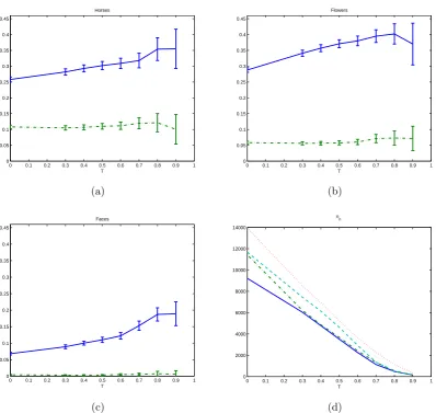
Figure 3.2 (a), (b) and (c) show these plots for the horses, yellow flowers and faces datasets respectively. The positive classificationspp improves as the saliency threshold

increases for all objects (with 0 ≤ T ≤ 0.8). The improvement with saliency (T= 0.8) versus without saliency (T=0) is of 10% for Horses, 12% for Flowers, and 12% for Faces. This seems to indicate that the feature points that are left out for classification asTincreases are more often fromC¯ (background) than the class of interestC(horse, flower, face). On the other hand, the (false positive) proportion 1−pn measuring the

proportion of points classified in C in the negative set of images (where no object of interest appears) remains more or less constant whatever the saliency level chosen.

This first result indicates that selecting features using saliency will not deteriorate classification performances but can in fact improve them.

As the saliency threshold increases, the standard errors for the proportions also increase. This is due to the fact that the number of selected features, np and nn,

decrease while the proportions, pp and pn, increase (and hence so does p(1−p)) as T

increases (see Equation 3.2). Therefore, althoughppgenerally improves as the threshold

increases, the certainty about how much the proportion actually improves is reduced. It can also be noticed that the standard errors for faces are smaller at each value of T compared to the other two classes. The reason for this is that more feature points were being detected in this class of images as opposed to flower and horse images (cf. Figure 3.2 (d)). Most of the face images were taken with relatively ‘busy’ backgrounds that foster bountiful amounts of feature point detection. The difference in the number of feature points detected in the three classes can also explain the lowpp values obtained

for the faces dataset. More background points will bring down the value ofpp.

It should also be noted that variations in numbers of feature points can occur in images in the same class and not just across classes. This can be noticed in Figure 3.3. The yellow flower, for example, on the left has significantly less feature points than the flower on the right.

(54)

0 0.1 0.2 0.3 0.4 0.5 0.6 0.7 0.8 0.9 1 0 0.05 0.1 0.15 0.2 0.25 0.3 0.35 0.4 0.45 Horses T (a)

0 0.1 0.2 0.3 0.4 0.5 0.6 0.7 0.8 0.9 1 0 0.05 0.1 0.15 0.2 0.25 0.3 0.35 0.4 0.45 Flowers T (b)

0 0.1 0.2 0.3 0.4 0.5 0.6 0.7 0.8 0.9 1 0 0.05 0.1 0.15 0.2 0.25 0.3 0.35 0.4 0.45 T Faces (c)

[image:54.595.122.521.183.560.2]

0 0.1 0.2 0.3 0.4 0.5 0.6 0.7 0.8 0.9 1 0 2000 4000 6000 8000 10000 12000 14000 T n n (d)

Figure 3.2: (a): proportion of correct classification for the horses datasetpp (solid blue

line) and 1−pn (green dashdot line) w.r.t. T; (b) proportion of correct classification

for the flowers dataset pp (solid blue line) and 1−pn (green dashdot line) w.r.t. T; (c)

proportion of correct classification for the faces datasetpp (solid blue line) and 1−pn

(green dashdot line) w.r.t. T; (d) total no. of feature points np for horses (solid blue

line), flowers (green dashdot line) and faces (dotted red line) and nn (aqua dashed

(55)

[image:55.595.108.533.152.375.2]

as the saliency threshold increases.

Figure 3.3: Example results forT = 0.3 and 0.6. From top to bottom: horses, flowers and faces. Green dots indicate feature points classified in the image class (C), purple dots indicate feature points classified outside of it (C).¯

3.3.2 Disk Space Usage Results and Discussion

Another aspect of this experiment was to see what effect changing the value of Twould have on disk space usage and classification time. Figure 3.4 (a) shows a plot of the memory usage required for storing feature points in memory for the three classes of images. A SURF feature point is a 64 element vector of floating point numbers. Since the size of doubles stored in memory is machine dependent, a single unit of memory usage was used for a double to abstract over this machine dependence (1 double = 1 unit, 1 SURF feature point = 64 units).

Figure 3.4 (a) depicts a clear downward trend for memory usage for all three classes. This trend is linear untilT = 0.7 when the rate of change decreases. At T = 0.5, for example, a 60% decrease in required memory usage is obtained, while a 75% result is obtained at threshold value 0.6.

Visual attention using 2D & 3D displays