International Journal of Emerging Technology and Advanced Engineering
Website: www.ijetae.com (ISSN 2250-2459,ISO 9001:2008 Certified Journal, Volume 3, Issue 5, May 2013)
1
Determination of Optimal Parameters in a Wavelet Collocation
Method
Marco Schuchmann
1, Michael Rasguljajew
21,2
Mathematical Faculty, University of Applied Science, Darmstadt, Hesse, Germany
Abstract— This article describes the setting of the parameters in a wavelet collocation method which minimizes the sum of squares of residuals. In a research project several different types of differential equations were approximated with this method. A lot of parameters must be adjusted in the discussed method here. Parameters are the number of collocation points, the number of base elements, which will be considered in the approximation and the resolution index j
(also known as the detail parameter). An important question is how to assess an approximation, if we don't know the exact solution. By using the Shannon wavelet we have additional information about the parameter j with respect to the Fourier space. The advantage of the wavelet collocation is its universal application possibility on different types of differential equations. In this article we show in examples, how we can detect a too small parameter j and how to recognize if we have not enough collocation points. With the fast discrete wavelet collocation we can - under certain conditions - assess the change of the approximation from the resolution j-1 to the resolution j. In examples we show how to detect a too small j
or a too small number of collocation points. The last chapter deals with the description of the algorithm.
Index Terms—ODE, sinc collocation, Shannon wavelet, wavelet collocation,
I. INTRODUCTION
In the wavelet theory a scaling function is used, which has properties that are defined in the MSA (multi scale analysis). Through the MSA we know, that we can construct an orthonormal basis of a closed subspace Vj, where Vj belongs to a sequence of subspaces with the
following property:
... V1 V0 V1... L2(R),
{j,k(t)}kZ is an orthonormal basis of Vj with j,k(t) =
2j/2(2jt - k).
We use the following approximation function:
(
)
:
,(
)
max
min
t
c
t
y
jkk
k k
k
j
, with C1(Z).
kmax and kmin depend on the approximation interval [t0,tend].
Now we can approximate the solution of an initial value problem y' = f(y,t) and y(t0) = y0 by minimizing the
following function
(1)
2 2 0 0 1
2
2
(
)
)
),
(
(
)
(
'
)
(
c
y
t
f
y
t
t
y
t
y
Q
jm
i
i i j i
j
For m = |kmax - kmin| we get an equivalent problem:
)
),
(
(
)
(
'
i j i ij
t
f
y
t
t
y
, with i = 1, 2, ...., mand
y
j(
t
0)
y
0.The advantage of calculating c by minimizing Q is that we can choose more collocation points tias shown in the
following example. In that case we apply the least squares
method to calculate c. Many simulations had shown that if
Qmin is very small then the approximation yj is good. An
even better criterion for a good approximation yjis Qa (see
(3)). Moreover, the equations have been ill-conditioned in several examples.
Analogously we could use boundary conditions instead of the initial conditions. This method can be even used analogously for PDEs, ODEs of higher order or DAEs, which have the Form F(
y
'
,
y
,
t
)
0
.In the following example, we use this method for the calculation of c.
If y' = f(y,t) is an ODE system, then we use the approximation function:
T k
k k
k j n k k
k k
k j k k
k k
k j k j
t
c
t
c
t
c
t
y
f
max
min max
min max
min
)
(
,
..
,..
)
(
,
)
(
)
(
, ,
, 2 , ,
1 ,
International Journal of Emerging Technology and Advanced Engineering
Website: www.ijetae.com (ISSN 2250-2459,ISO 9001:2008 Certified Journal, Volume 3, Issue 5, May 2013)
2
For the i-th component of the solution y, we use as usual the notation yi. We use for the i-th component of yj the
notation yj(i), in order not to lead to a confusion with the
approximation yj out of Vj, so it will be always
distinguished whether the approximation yj or the i-th
component of y is used.
We use the collocation points ti, with ti = t0 + ih and
(2)
m
t
t
h
end
0(m ≥ |kmax - kmin|).
Simulations have shown that even with m < |kmax - kmin|
we getgood approximations.
For the assessment of the approximation we use the value Qa, with
(3)
2 2 0 0 1
2
2
(
)
)
),
(
(
)
(
'
f
y
y
t
y
y
Q
jm
i
i i j i
j a
a
i = t0 + ih/a, ma = am and a >1 is an integer.
In the examples we use the Shannon wavelet. Although it has no compact support and no high order, in many examples and simulations we got a much better approximation than using other wavelets (f.e. Daubechies
wavelets of order 5 to 8), even with a small n. The Meyer
wavelet yields good results, too. We even get a good extrapolation outside the interval [t0, tend].
Additional benefits of the Shannon wavelets:
(a) The Shannon wavelet is analytically defined as the scaling function is.
(b) Both Shannon wavelet and scaling function are indefinitely often differentiable (see [34]).
(c) The scaling function is band limited and we can "generalize" the sampling theorem of Shannon.
(d) The scaling function has properties that as scaling functions of so-called interpolating wavelets have. (See definition Donoho in 1992 [19] or [41]) this includes (kZ):
(i)
else
k
for
k
0
0
1
)
(
(ii)
k
k
t
k
t
)
(
/
2
)
(
2
)
(
(ii) follows from the Shannon sampling theorem, so we can calculate the filter coefficients of the scaling equation with the function values (k/2).
About interpolating wavelets there are a number of publications with error estimates and also for the approximation of the solutions of initial value problems and boundary value problems (for ordinary and partial differential equations) see [45], [8], [46], as well as to the sinc collocation method (see [15], [1], [33]) with special collocation points ("sinc grid points", see [33]).
In [30] a quasi Shannon wavelet is used to approximate the solution of a boundary value problem (with an ordinary differential equation). Here, the scaling function of the Shannon wavelet is weighted with the gauss function
) 2 /( 2 2
)
(
t
e
tR
, so that the decay of the scalingfunction is improved.
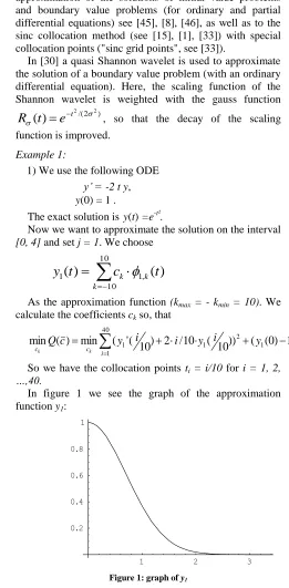
Example 1:
1) We use the following ODE
y’ = -2 t y, y(0) = 1 .
The exact solution is y(t) =e-t².
Now we want to approximate the solution on the interval
[0, 4] and set j = 1. We choose
1010 , 1
1
(
)
(
)
k
k
k
t
c
t
y
As the approximation function (kmax = - kmin = 10). We
calculate the coefficients ck so, that
2 1 2 1 40
1
1
'
(
10
)
2
/
10
(
10
))
(
(
0
)
1
)
(
min
)
(
min
y
i
y
i
i
y
c
Q
i c
ck k
So we have the collocation points ti = i/10 for i = 1, 2, …,40.
In figure 1 we see the graph of the approximation function y1:
1 2 3 4
0.2 0.4 0.6 0.8 1
[image:2.612.310.571.153.684.2]International Journal of Emerging Technology and Advanced Engineering
Website: www.ijetae.com (ISSN 2250-2459,ISO 9001:2008 Certified Journal, Volume 3, Issue 5, May 2013)
3
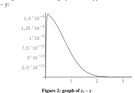
In figure 2 we see the graph of the approximation error
y1 – y:
1 2 3 4
2.5´10-10 5´10-10 7.5´10-10 1´10-9 1.25´10-9 1.5´10-9
[image:3.612.58.281.132.286.2]Figure 2: graph of y1 – y
In simulations we saw, that for a function which is not in 2(R) we get with the coefficients c
k a better approximation
than with
(4)
y
(
t
)
(
t
)
dt
f
,kj
k
1on the interval I = [t0, tend] if we use I for the integration
interval to calculate fk1 (see [38] and Remark 4). Remark 1:
With the Shannon theorem we can construct an approximation that is bandlimited with
supp(Y) =
|
With the function
k
k
t
b
y
k k
π
t
Ω
)
π
sin(Ω
(t)
.
Practically, we must limit the summation range again ({k| kmin≤ k ≤ kmax}).
When the solution y is band limited with supp(Y)
|
, then the coefficients can be calculated with function values
y
(t)
=y
(t)
andk
)
Ω
π
(
y
b
k
,Which follows with the sample theorem. If we, as in the in the following examples, construct the approximation
function yj with the scaling function of the Shannon
wavelet, then
= 2j. So y is in Vj if
supp(Y)
[-2j, 2j] .If the exact solution is band limited, then ck = 2-j/2bk,
that means that fkj = 2-j/2y(k/2j). Even if the function is not
band limited, we get fk j
2-j/2y(k/2j), if j is not too small. II. THE CHOICE OF THE PARAMETER AND THE
ASSESSMENT OF THE APPROXIMATION
Here are some considerations about the setting of the parameter kmin und kmax, j and m.
The choice of kmin and kmax:
Generally the summation area depends on the approximation interval I = [t0, tend].
If the scaling function
has a compact support, we canchoose
k
max andk
minso, that
j,k(
t
)
0
For t I and
k
k
max,k
k
min.If the support of the scaling function
is not compact (or if the support is compact, but the function values are on a part of I very small), we choose kmin and kmax so, that
j,k(
t
)
For t I and
k
k
max,k
k
min with a
> 0.Remark 2:
In simulations the approximation was not so sensitive to the choice of kmin and kmax and even with few coefficients ck
we got a good approximation with the Shannon wavelet, although it has not a compact support and it decreases not very fast.
The choice for the parameter j:
If j is too small (and if we have enough collocation points or m is big enough), then the ODE is not nearly well fulfilled. If yj is the exact solution, then
Qmin = min Q(c) = 0
Thus we can see from the minimum value of Q or Qmin,
whether j is too large. Later we will see that we can assess the approximation with Qmin (or even better with Qa, see
(3)) even if h is small enough.
As an example we choose an easy ODE only to show that we can see by looking at Qminif j is too small.
Example 2:
)
10
cos(
10
)
(
'
t
t
y
,International Journal of Emerging Technology and Advanced Engineering
Website: www.ijetae.com (ISSN 2250-2459,ISO 9001:2008 Certified Journal, Volume 3, Issue 5, May 2013)
4
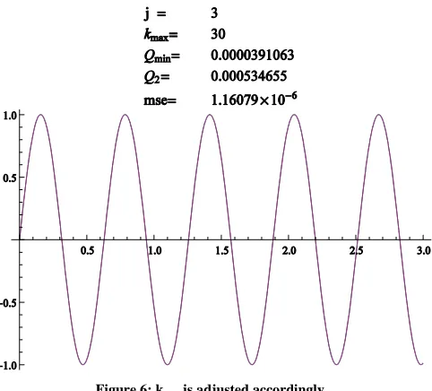
The exact solution y is V2. We use the approximation
interval I = [0, 3] and set h = 3/(2kmax), ti = ih (with i = 1, 2, …, 2kmax)and -kmin = kmax. We now see the graphs of yj
and the exact solution y (with y(t) = sin(10t)) for kmax = 15, 20, 30 and j = 1, 2, 3. With j = 1 all values of Qminhave
been relatively big. In the graphs we see the mean square error (mse) calculated with
2 100
0
)
)
100
/
3
(
)
100
/
3
(
(
101
1
i
j
i
y
i
y
mse
. [image:4.612.44.581.84.666.2]With j = 3 we even see, that kmax is too small, as the following graphs show:
[image:4.612.251.557.104.561.2]Figure 3: j is too small
Figure 4: good results; j is set well
[image:4.612.50.298.274.475.2]International Journal of Emerging Technology and Advanced Engineering
Website: www.ijetae.com (ISSN 2250-2459,ISO 9001:2008 Certified Journal, Volume 3, Issue 5, May 2013)
[image:5.612.51.292.120.338.2]5
Figure 6: kmax is adjusted accordingly
Remark 1 also gives us an indication of the meaning of the choice of j with respect to the frequency domain.
The choice of the parameter m (number of collocation points):
First be noted that we have chosen the equidistant collocation points in all examples. In problems with a fast changing function in a part of the approximation interval (as in stiff problems), we could choose a smaller step size for this part. When curves are almost asymptotically or approximately linear, we can use a greater step size.
With the minimization of Q we minimize the residuals at
the collocation points. But for a good approximation, the residuals should be small at all points. Because we get as approximation a whole function (not only points), we can calculate the residuals at other points. Because of this reason we use the function
d
(
t
)
(
y
j'
(
t
)
f
(
y
j(
t
),
t
))
2to see if the approximation is good in other points.
If the function values at point t with t
ti of d arerelative big, we need more collocation points in Q. For that assessment we don’t even need a second minimization.
If we choose in example 1 m = 8, we get the following
graph of d:
1 2 3 4
1 2 3 4 5 6 7
Figure 7: graph of d with m = 8 (example 1)
So we can compare as a criterion Qmin with Qa. For a
bigger parameter a we could weight Qa with 1/a for a
comparison, but in many simulations we got good results with a = 2.
If Qa >> Qmin we should choose a bigger m.
As a starting value for m a good choice is m = |kmax - kmin| (see (1)); this has been even confirmed in many
simulation. For extreme stiff problems with big slopes or curvatures (not only because of the stiffness) we need a bigger m (and even a bigger j).
Remark 3 for the choice of m:
1) Important for the choice of the number of collocation points m is the behaviour of the solution, as for any implicit or explicit method in general. Here we even could divide the approximation interval or use different step size.
2) If we use the Shannon wavelet, because of the Shannon theorem, we could choose m so that
j i
i
t
t
t
1
2
. For t j ii
2 all coefficients ck in yj
will vanish, because
else
i
for
i
0
0
1
)
(
and so
else
k
i
for
i
j j
k j
0
2
)
2
(
2 / ,
[image:5.612.322.563.124.308.2]International Journal of Emerging Technology and Advanced Engineering
Website: www.ijetae.com (ISSN 2250-2459,ISO 9001:2008 Certified Journal, Volume 3, Issue 5, May 2013)
6
For the derivation of at the points
t
i
j
i
2
we get:
else
k
i
for
i
k/
)
1
(
0
0
)
(
'
If we increase j by 1, we should halve
t
, in order to consider the "Details" for larger j.Remark 4 for the choice of j:
1) By using the discrete wavelet transform from Mallat we could approximately compare ckj-1 with ckj. For that
comparison we don’t even have to minimize twice if the approximation for yjis not too bad (if Qa is small). Here is
the algorithm of Mallat:
(5) fkj-1 =<y, j-1,k >=
j k j
k
y
h
f
h
ll l l
l
l
2
,
,
2 ,(6)dk j-1
=<y,j-1,k>=
j k j
k
y
g
f
g
ll l l
l
l
2
,
,
2 ,with hk = <,1,k> and k k
k
h
g
(
1
)
1 .With this we can calculate the coefficients dkj-1 and fkj-1
with the coefficients fkj. When we use the coefficients ckj as
an approximation of fkj we should not use the coefficients at
the edges.
With the Parseval theorem we get
k j k L
j
d
d
2 2 and
k j k L
j
f
y
2 2and because of the orthogonality (
d
j,
y
j
0
) we get:1 22
L j
y
= 22 22 22L j L j L
j
j
y
d
y
d
If we want to assess the change from yj-1 to yj, we can
calculate:
(7)
k j k k
j k
L j
L j
j
f
d
y
d
b
2 2 1 1
1
2 2
:
or
2 2 2
2 1 2
1
:
L j
L j L j
j
y
y
y
b
This idea was tested in simulations. We saw, that the effort of a DWT is not necessary because we can make a good assessment of the approximation with Qa and there
can be deviations between ck and fkj or the solution could not be in 2(R) like in most cases. In these cases we got also good approximations.
For a theoretical multi resolution analysis we could consider 1Iy instead of y, because when y is in 2(I) then 1Iy is in
2
(R), if we need an approximation on I. Here 1I is
the indicator function of the interval I.
In simulations we compared the approximation yj
calculated by the minimization of Q with an approximation
by an orthogonal projection of 1I y on. Here the
approximation yj for y on I (calculated by the minimization
of Q) was much better than the orthogonal projection of
1Iy on Vj and we could even get a good extrapolation
(outside the interval I).
In figure 4 we calculated fkj =
1
0,1y
,
j,k with y(t) =e-t and j = 3 to get an approximation of y on I and we see the graphs of y and yjby setting ck= fkj (kmax= - kmin = 24, y
is dashed):
0.2 0.4 0.6 0.8 1.0
[image:6.612.323.565.386.547.2]0.4 0.6 0.8 1.0
Figure 8: graph of y (dashed) and yj
With the orthogonal projection we project the function yj
(by setting ck = fkj) on a function, which is equal to zero
outside I.
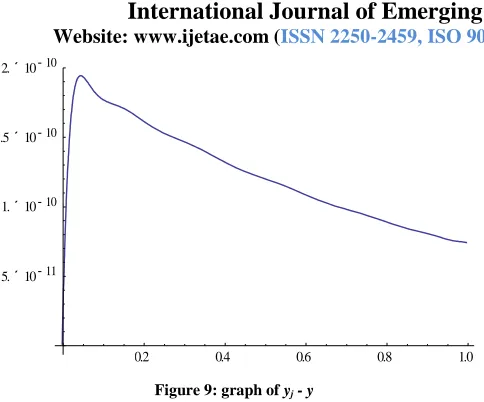
But if we approximate the Solution of the ODE y´= -y,
y(0) = 1, with kmin = -8 and kmax = 10, j = 1 and
collocation points ti = i/20 with i = 1, 2, ..., 20 to get an
International Journal of Emerging Technology and Advanced Engineering
Website: www.ijetae.com (ISSN 2250-2459,ISO 9001:2008 Certified Journal, Volume 3, Issue 5, May 2013)
7
0.2 0.4 0.6 0.8 1.0
[image:7.612.51.293.93.294.2]5.´10-11 1.´10-10 1.5´10-10 2.´10-10
Figure 9: graph of yj - y
We can even use the function yj for an extrapolation.
Below is the graph of yj - y on a bigger area than I for an
extrapolation:
-0.5 0.5 1.0 1.5
[image:7.612.47.289.338.515.2]-0.0001 -0.00008 -0.00006 -0.00004 -0.00002
Figure 10: graph of yj - y
With a smaller j and a smaller |kmax - kmin| we get a much
better approximation.
2) Now we see the error of the approximation with the Shannon wavelet by using the information about the Fourier space. There we see that for a good approximation with the Shannon wavelet the decay behaviour of Y() is important. This is what we see if we take a look at the differences of y and yj by considering the Fourier transform
(yj is here the orthogonal projection of y in Vj).
y(t) - yj(t) =
j
j
d
e
Y
d
e
Y
i t i t2
2
)
(
2
1
)
(
2
1
jj
d
e
Y
d
e
Y
i t i t2 2
)
(
2
1
)
(
2
1
With the Parseval equation:
2 L j
y
y
j j
d
Y
d
Y
2
2 2
2
)
(
)
(
There we see, that it is important that |Y()| becomes small quickly, in order to get a good approximation with a small j.
Analogously we get:
2 L j
d
1
1
2
2
2 2
2
2
)
(
)
(
j
j j
j
d
Y
d
Y
With the Riemann-Lebesgue Theorem we get:
lim
2
0
j L
j
d
As Y() approaches zero with increasing || the detail coefficients dkjapproache to zero with bigger j. The faster Y() approaches to zero the better the approximations gets with a small j.
With the wavelet collocation we have some advantages:
1) We get an approximation function and not only points and we can adjust with j the details we want to consider. The approximation function can also be used for an extrapolation.
2) If we have an inverse problem or a general approximation, we do not need to specify a special type of function.
3) The ODE doesn’t have to be given in an explicit form
y´ = f(y,t), and we don’t need an initial value y(t0) = y0, we
could also use y() = y with [t0, tend]. We can even
approximate solutions of higher order ODEs, with boundary values, DAEs or PDEs.
Remarks 5:
International Journal of Emerging Technology and Advanced Engineering
Website: www.ijetae.com (ISSN 2250-2459,ISO 9001:2008 Certified Journal, Volume 3, Issue 5, May 2013)
8
2) With a bigger j we need a bigger |kmax - kmin| and thus a
bigger m. The reason is that with increasing j we compress the function
j,k.3) With Qa we could see in all simulations, if the
approximation ist good. We got a linear correlation between ln(Q2) and ln(mse) in all simulations. In figure 7
we see the graph of a linear regression (with a R squared of 0.998) of ln(mse) against ln(Q2) with the points (ln(Q2), ln(mse)), which have been calculated with different j (j = 0, 1, 2), kmin = - kmax (kmax = 15, 20, 25) and m (m = kmax, 2kmax,
3kmax) with the ODE and I of the example 1.
-50 -40 -30 -20 -10
[image:8.612.48.288.264.420.2]-60 -50 -40 -30 -20 -10
Figure 11: linear regression plot of ln(mse) against ln(Q2)
III. THE ALGORITHM
Here is a adaptive algorithm for the adjustment of j und
m:
Algorithm:
Without additional information we set j = 1 and m =
|kmax - kmin|. kmin and kmax depend on the approximation
interval. We calculate Qmin and Q2.
If Qmin < 1 we test if Q2 < 2with suitable 1 and 2
(graphically we could consider d).
When both conditions are fulfilled the iteration stops. If Qmin < 1is not fulfilled, we increase j by one.
If Qmin < 1is fulfilled and Q2 < 2not, we increase m. Remark 7:
If the function y has very big slopes in the beginning of the approximation interval I, as with stiff problems, we can begin with a bigger i than 1 (here i0) in the calculation of Q2:
2 2 0 0 2
2
(
)
)
),
(
(
)
(
'
0
y
t
y
y
f
y
Q
jm
i i
i i j i
j a
a
In the simulations with such functions we saw, that the residuals can be very big with
i at the beginning of the interval I, although the approximation outside around t0 isvery good and the residuals are very small here.
REFERENCES
[1] Abdella, K. (2012). “Numerical Solution of two-point boundary value problems using Sinc interpolation,” Proceedings of the American Conference on Applied Mathematics (American-Math '12): Applied Mathematics in Electrical and Computer Engineering [2] Ascher, U. A. Mattheij, R. M. M. Russell, R. D. (1988).
„Numerical Solution of Boundary Value Problems for ODEs, ” Prentice Hall (Series in Computational Mathematics)
[3] Ascher, U. Christiansen, J. Russell, R. (1981). “Collocation Software for Boundary Value ODEs,” ACM Trans. Math. Software [4] Bauer, I. Bock, H. G. Körkel, S. Schlöder, J. P. (2000). „Numerical
Methods for Optimum Experimental Design in DAE Systems,” Journal of Computational and Applied Mathematics
[5] Biegler, L. T. (1984). “Solution of Dynamic Optimization Problems by Successive Quadratic Programming and Orthogonal Collocation,” Comput. Chem. Engng.
[6] Biegler, L. T. (2002). “Advances in Simultaneous Strategies for Dynamic Systems,” Chemical Engineering Sciences
[7] Binder, T. Blank, L. Bock, H. G. Burlisch, R. et. al. (2001). “Introduction to Model Based Optimization of Chemical Processes on Moving Horizons,” In: Online Optimization of Large Scale Systems” Springer Verlag
[8] Bertoluzza S. (2006). “Adaptive wavelet collocation method for the solution of Burgers equation,” Transport Theory and Statistical Physics, 25: 3-5
[9] Bock, H. G. (1978). “Numerical Solution of Nonlinear Multipoint Boundary Value Problems with Application to Optimal Control,” Z. Angew. Math. Mech.
[10] Bock, H. G. (1981) . “Numerical Treatment of Inverse Problems in Chemical Reaction Systems,” Springer Series in Chem. Phys. [11] Bock, H. G. (1983) . “Recent Advances in Parameter Identification
Techniques for ODE,” Numerical Treatment of Inverse Problems in Differential and Integral Equations (P. Deuflhard und E. Hairer Ed.) Birkhäuser
[12] Bock, H. G. (1987) . „Randwertproblemmethoden zur Parameteridentifizierung in Systemen nichtlinearer Differentialgleichungen,“ Bonner Mathematische Schriften Nr. 183 [13] Bock, H. G. Eich. E. Schlöder, J. P. (1988) . „Numerical Solution
of Constrained Least Squares Boundary Value Problems in DAE,” in “Numerical Treatment of Differential Equations” BG Teubner Leipzig
[14] Bock, H. G. Schlöder, J. P. (1987) . “Recent Progress in the Development of Algorithms and Software for Large Scale Parameter Estimation Problems in Chemical Reaktion Systems,” Preprint 441, Research Report (123/256) Univerity Bonn/ Univerity Heidelberg [15] Carlson, T. S. Dockery, J. Lund, J. (1997). “A Sinc-Collocation
Method for Initial Value Problems,” Mathematics and Computation, Vol. 66, No. 217
International Journal of Emerging Technology and Advanced Engineering
Website: www.ijetae.com (ISSN 2250-2459,ISO 9001:2008 Certified Journal, Volume 3, Issue 5, May 2013)
9
[17] Deuflhard, P. Hairer, E. (1983). “Numerical Treatment of Inverse Problems in Differential and Integral Equations,” Band 2 Birkhäuser [18] Diehl, M. Bock, H. G. Schlöder, J. P. Findeisen, R. Nagg, Z. Allgöwer, F. (2002). „Real – Time Optimization and Nonlinear Model Predictive Control of Processes Governed by DAEs,” Journal of process control Vol.12, No. 4
[19] Donoho, D. L.; (1992). “Interpolating Wavelet Transforms,” Tech. Rept. 408. Department of Statistics, Stanford University, Stanford [20] Ebert, K. H. Deuflhard, P. Jaeger, W. (Ed.) (1981). “Modelling of
Chemical Reaction Systems,” Springer Ser. Chem. Phys. 18 [21] Fogler, H. S. (1999). “Elements of Chemical Reaction Engineering,”
3. Auflage Prentice Hall International Series in the Physical and Chemical Engineering Sciences
[22] Guay, M. McLean, D. D. (1995). “Optimization and Sensitivity Analysis for Multiresponse Parameter Estimation in Systems of ODEs,” Computers and Chemical Engineering
[23] Hairer, E. Wanner, G. (1993). Vol. 1 : “Nonstiff Problems,” Springer 2. Auflage
[24] Hairer, E. Wanner, G. (1996). Vol. 2 : “Stiff and Differential-Algebraic Problems,” Springer 2. Auflage
[25] Kameswaran, S. Biegler, L. T. (2006). „Simultaneous Dynamic Optimization Strategies: Recent Advances and Challenges,” Computers and Chemical Engineering
[26] Kiehl, M. (1998). “Sensitivity Analysis of Stiff and Non-Stiff Initial-Value Problems,” International Series of Numerical Mathematics Birkhäuser Verlag Basel
[27] Leineweber, D. B. Bock, H. G. Schlöder, J. P. et al. (1997). “A Boundary Value Approach to the Optimization of Chemical Process Described by DAE Models,” Computers and Chemical Engineering [28] Lohmann, T. Bock, H. G. Schlöder, J. P. (1992). „Numerical
Methods for Parameter Estimation and Optimal Experiment Design in Chemical Reaction Systems,” Ind. Eng. Chem. Res.
[29] Lohmann, T. W. (1999). “Modelling and Parameter Estimation of Reaction Kinetics and Coal Pyrolysis,” Journal of Inverse and Ill Posed Problems Vol. 7
[30] Mei, S.-L. Lv, H.-L. Ma, Q. (2008). „Construction of Interval Wavelet Based on Restricted Variational Principle and Its Application for Solving Differential Equations,” Hindawi Publishing Corporation Mathematical Problems in Engineering
[31] Nowak, U. Deuflhard, P. (1985). “Numerical Identification of Selected Rate Constants in Large Chemical Reaction Systems,” Appl. Num. Math. 1
[32] Nowak, U. Deuflhard, P. (1986). “Efficient Numerical Simulation and Identification of Large Chemical Reaction Systems,” Preprint SC-86-1 des Konrad Zuse-Zentrums für Informationstechnik Berlin (ZIB)
[33] Nurmuhammada, A. Muhammada, M., Moria, M. Sugiharab, M. (2005). “Double exponential transformation in the Sinc-collocation method for a boundary value problem with fourth-order ordinary differential equation,” Journal of Computational and Applied Mathematics
[34] Qian, L. (2002). “On the Regularized Whittaker-Koltel'nikov-Shannon Sampling Theorem,” Proceedings of the Amarican Mathematical Society, Vol. 131, No. 4
[35] Robertson, H. H. (1975). “Some Properties of Algorithms for Stiff Differential Equations,” J. Inst. Math. Applics.
[36] Russell, R. D. Christiansen, J. (1979). “A Collocation Solver for Mixed Order Systems of Boundary Value Problems,” Mathematics of Computation
[37] Schuchmann, M. (2012). “Approximation and Collocation with Wavelets. Approximations and Numerical Solving of ODEs, PDEs and IEs,” Osnabrück: DAV
[38] Schuchmann, M. Rasgulajajw, M. (2013). “An Approximation on a Compact Interval Calculated with a Wavelet Collocation Method can Lead to Much Better Results than other Methods,” Journal of Approximation Theory and Applied Mathematics, Vol. 1, 2013 [39] Schulz, V. H. Bock, H. G. Steinbach, M. C. (1998). „Exploiting
Invariants in the Numerical Solution of Multipoint Boundary Value Problems for DAE,” Siam Journals Online
[40] Scitovski, R. Jukic, D. (1996). “A Method for Solving the Parameter Identification Problem for ODEs of the second Order,” Applied Mathematics and Computation - Elsevier
[41] Shi, Z.; Kouri, D.J.; Wei, G.W.; Hoffman, D. K.; (1999). „Generalized Symmetric Interpolating Wavelets,” Computer Physics Communications
[42] Strang, G.; (1989). “Wavelets and Dilation Equations: A Brief Introduction,” SIAM Review Vil. 31, No. 4
[43] Unser, M. (1996). “Vanishing moments and the approximation power of wavelet expansions,” Proceedings of the 1996 IEEE International Conference on Image Processing
[44] Unser, M. Blu, T. (1998). “Comparison of Wavelets from the Point of View of their Approximation Error,” Proc. Of SPIE Vol. 3458, Wavelet Applications in Signal and Image Processing
[45] Vasilyev, O. V.; Bowman, C.; (2000). “Second-Generation Wavelet Collocation Method for the Solution of Partial Differential Equations,” Academic Press