Pattern discovery in time oriented data

Pattern discovery in time­oriented data

Saraee, MH, Theodoulidis, B and Koundourakis, G

Title Pattern discovery in time­oriented data

Authors Saraee, MH, Theodoulidis, B and Koundourakis, G

Type Conference or Workshop Item

URL This version is available at: http://usir.salford.ac.uk/18698/

Published Date 1998

USIR is a digital collection of the research output of the University of Salford. Where copyright  permits, full text material held in the repository is made freely available online and can be read,  downloaded and copied for non­commercial private study or research purposes. Please check the  manuscript for any further copyright restrictions.

PATTERN DISCOVERY IN TIME-ORIENTED DATA

Mohammad Saraee, George Koundourakis and Babis Theodoulidis

TimeLab

Information Management Group Department of Computation,

UMIST, Manchester, UK

Email: saraee, koundour, babis@co.umist.ac.uk

ABSTRACT

We present a data mining system, EasyMiner which has been developed for interactive mining of interesting patterns in time-oriented databases. This system implements a wide spectrum of data mining functions, including generalisation, characterisation, classification, association and relevant analysis. By enhancing several interesting data mining techniques, including attribute induction and association rule mining to handle time-oriented data the system provide a user friendly, interactive data mining environment with good performance. These algorithms were tested on time-oriented medical data and experimental results show that the algorithms are efficient and effective for discovery of pattern in databases.

INTRODUCTION

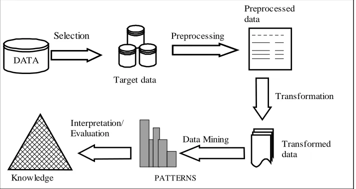
Knowledge Discovery in Databases (KDD) is the effort to understand, analyse, and eventually make use of the huge volume of data available. According to Fayyad et al. [1] KDD is the non trivial process of identifying valid, novel, potentially useful, and ultimately understandable patterns in data. In their opinion, there are usually many steps in a KDD process including selection, pre-processing, transformation, data mining, and interpretation/ evaluation of the results as shown in Figure 1. As seen in the Figure data mining is only one step of the process, involving the application of discovery tools to find interesting patterns from targeted data, but in the research community most often the term data mining and KDD have been used interchangeably

.

But in many situations, this snapshot-type of database is inadequate. They cannot handle queries related to any historical data. For many applications such as accounting, banking, GIS systems and medical data the changes made their databases over time are a valuable source of information which can direct their future operation. The pattern discovered from conventional databases has limited value since the temporal nature of data is not taken into account but only the current or latest snapshot.

[image:3.612.111.467.257.446.2]

In the rest of the paper the data mining techniques used by Easy Miner for discovering interesting patterns from time-oriented database are described. In section 2 relevance analysis method is presented with examples from medical domain. In section 3 association rules mining technique is presented and section 4 describes Easy Miner approach to pattern discovery by mining classification rules. Section 5 concludes with a summary of the paper and outline of the future work.

Figure 1. The knowledge discovery process

1

Relevance Analysis

As we know from real life, several facts are relevant with each other and there is a strong dependence between them, for example Age is relevant to Date of Birth, Title(Mr, Mrs, Miss) is relevant to Sex and Marital Status. This kind of knowledge is qualitative and it is quite useful to mine it from large databases that hold information about many objects(fields). For example a bank could look in its data and identify which are the factors that it should take in mind in order to give a Credit Limit to a customer. As we found by using EasyMiner Credit Limit is relevant to

Account Status, Monthly Expenses, Marital Status, Monthly Income, Sex and etc.

A number of statistical and machine learning techniques for relevance analysis have been proposed until now. The most popular and acceptable approach in the data mining community, is the method of measuring the uncertainty coefficient[4].

Let us suppose that the generated set from the collection of task relevant data is a set P of p data records. Suppose also, that the interesting attribute has m distinct values defining by this way m

Knowledge DATA

Selection

Target data

Preprocessing

Data Mining

Transformation

PATTERNS

Interpretation/ Evaluation

Preprocessed data

discrete classes Pi (i=1,…, m). If P contains pi records for each Pi, then a random selected record

belongs to class Pi with probability pi/p. The expected information needed to classify a given

sample is given by: I p p p p p

p p m

i i

i m

( ₁, ₂, . . , ) lo g₂

1

= −

=

∑

An attribute A with values {a1, a2,…, ak} can be used to partition P into {C1, C2,…, Ck}, where

Cj contains those records in C that have value aj of A. Let Cj contain pij records of class Pi. The

expected information based on the partitioning using as split attribute the A, is:

E A p p

p I p p

ij m j

ij m j j

k

( )= + +. . . ( + +. . . )

=

∑

1

So, the information gained by partitioning on attribute A is:

gain A

( )

=

I p p

( , ,...,

_{1 2}

p

_m

)

−

E A

( )

The uncertainty coefficient U(A) for attribute A is obtained by normalising the information gain of A so that U(A) ranges from 0 to 1. The value 0 means that there is significant independence between the A and the interesting attribute, and 1 means that there is strong relevance between the two attributes. The normalisation of U(A) is achieved by the following equation:

U A I p p p E A

I p p p

m

m ( ) ( , ,..., ) ( )

( , ,..., )

= 1 2 −

1 2

It is upon the user to keep the n most relevant attributes, or all the attributes that have value of uncertainty coefficient greater than a pre-specified minimum threshold[4].

2

Classification

Classification is an essential issue in data mining. Classification partitions massive quantities of data into sets of common characteristics and properties[5],[6]. This procedure can be described as follows.

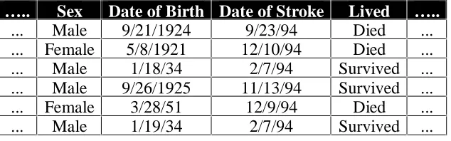
We are given a large population database that contains information about population instances. The population is known to comprise of m groups (classes), but the population instances are not labelled with the group identification. In addition, a population sample is given (much smaller than the population but representative of it) called training set. In this training set, each tuple is assumed to belong to a predefined class, as determined by one of its attributes, called class label. Figure 2 shows a part from a sample training set of the medical database, where each record represents a patient. The purpose of classification is to discover and analyse the rules that govern the training set, in order to apply them into the whole population of database and get the class label of every instance of it.

….. Sex Date of Birth Date of Stroke Lived …..

[image:4.612.155.472.588.687.2]

... Male 9/21/1924 9/23/94 Died ... ... Female 5/8/1921 12/10/94 Died ... ... Male 1/18/34 2/7/94 Survived ... ... Male 9/26/1925 11/13/94 Survived ... ... Female 3/28/51 12/9/94 Died ... ... Male 1/19/34 2/7/94 Survived ...

The classification technique that we have developed in Easy Miner is based on the decision tree structure. A decision tree is a flow chart structure consisting of internal nodes, leaf nodes and branches. Each internal node represents a test on an attribute and each branch represents the result of that test. Each leaf node represents a class (and in some cases classes).

By using a decision tree, untagged data sample can be classified. This can be done by testing the attribute values of the sample data against the decision tree. A path is produced from the root to a leaf node, which has the class identification of the sample.

2.2 Decision Tree Classifier

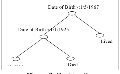
[image:5.612.203.403.313.437.2]

A decision tree is a class discriminator that recursively partitions the training set until each partition consists entirely or dominantly of examples from one class. Each non-leaf node of the tree contains a split point, which is a test on one or more attributes and determines how the data is partitioned. Figure 3 shows a sample decision-tree classifier based on the training set shown in Figure 2. This decision tree can be used in order to discriminate future patients that had stroke into Lived or Died categories.

Figure 3: Decision Tree

2.2.1 Characteristics of a Decision Tree Classifier

There are several simple characteristics in a decision tree classifier:

1. If a node is an internal one, then the left child node will inherit form it the data that satisfies the test of the node, and the right child node will inherit the data that does not satisfy the splitting test.

2. As we go down in the tree and the depth increases, the size of the data in nodes is decreasing and the probability that this data belongs to only one class increases.

3. Each node can have two or none children nodes. For this reason, it is obvious that the decision tree is a binary tree.

4. Because the decision tree is a binary tree, the number of internal nodes is (n-1)/2 and the number of leafs is (n+1)/2, where n is the total number of leafs in the decision tree.

5. Each path from the root to as leaf can be easily translated into IF-THEN rules

Lived

Died Date of Birth <1/1/1925

…… …

2.2.2 Collection of Training Set

In order to construct a decision tree classifier, the first step is to retrieve the classification task relevant data and store them in a relation (table). This is an ease task that executing a usual query can perform it.

The second step after collecting the classification task relevant data is to examine the generated training set with the purpose to “purify” it and make it suitable for input to the classification process. Including irrelevant attributes in the training set would slow down and possibly confuse the classification process. So the removal of them improves the classification efficiency and enhances the scalability of classification procedures by eliminating useless information and reducing the amount of data that is input to the classification stage. Therefore, relevance analysis is performed to the data set and then only the most n-relevant attributes are kept.

2.2.3 Construction of a Decision Tree Classifier

The algorithm that we are going to use for tree building is, in general, the following:

MakeTree(Tiraining Data T)

if (all points in S are in the same class) then return

EvaluateSplits( )

if (T can not be further partition) then Evaluate Each Class Probability(S) return

Use best split found to partition S into S1 and S2 Delete(S)

MakeTree(S1) MakeTree(S2)

The main points in this tree building algorithm are:

2.2.3.1Data Structures

For each attribute of the training data a separate list is created. An entry of the attribute list has the following fields: (i) attribute value, (ii) class label, (iii) index of the record (id) from which these value has been taken. Initial lists for numeric attributes are sorted when first created.

In the beginning, all the entries of the attribute lists are associated with the root of the tree. As the tree grows and nodes are split to create new ones, the attribute lists of each node are partitioned and associated with the children. When this happens, the order of the records in the list is preserved, so resorting is unnecessary and not required.

Other data structures that are used are histograms. These histograms are used to capture the class distribution of the attribute records at a given node. So, for numeric attributes, two histograms are associated with each decision-tree node that is under consideration for splitting Cabove and

a node an is called count matrix. So, for a numeric attribute the histogram is a list of pairs of the form <class, frequency> and for a categorical attribute, the histogram is a list of triples of the form <attribute value, class, frequency>.

2.2.3.2Evaluation of splits for each attribute

For the evaluation of alternative splits are used splitting indexes. Several splitting indexes are used for this purpose. Two of the most popular and acceptable indexes are the gini index and the

entropy index. Assuming that we have a data set T which contains examples from n classes and

where pj is the frequency of class j in data set T then gini(T) is:

gini T p_j

j n ( )= − =

∑

1 2 1

and the entropy index Ent(T) is:Ent T p_j p_j

j n

( )= − log ( ) =

∑

2

1

If a split divides S into subsets

S

₁ and

S

₂ , then the values of the indexes of the divided data are given by:

gini S n

n gini S n

n gini S split( )= ( )+ ( )

1

1 2

2 and Ent S n

n Ent S n

n Ent S split( )= ( )+ ( )

1

1 2

2

The advantage of these indexes is that their calculation requires only the distribution of the class values in each of the partitions.

To find the best split point for a node, we scan each of the attributes lists and evaluate splits based on that attribute. The attribute containing the split point with the lowest value for the split index (gini or entropy) is then used to split the node.

There are two kinds of attributes that we can perform a split:

•

Numeric attributes. If we have a numeric attribute A, a binary split A<u is performed to the

set of data that it belongs. The candidate-split points are midpoints between every two successive attribute values in the training data. In order to find the split for an attribute on a node, the histogram Cbelow is initialised to zeros whereas Cabove is initialised with the class distribution, for all the records for the node. For the root node, this distribution is obtained at the time of sorting. For the other nodes, this distribution is obtained when the node is created. Attribute records are read one at a time and Cbelow and Cabove are updated for each record read. After each record is read, a split between values we have and we have not yet seen is evaluated. Cbelow and Cabove have all the information to compute the gini or Entropy index. Since the lists for numeric attributes are kept in sorted order, each of the candidate split points for an attribute is evaluated in a simple scan of the associative attribute list. If a successful point is found, we save it and we de-allocate the Cbelow and Cabove histograms before we continue on the next attribute

•

Categorical Attributes. If S(A) is the set of possible values of a categorical attribute A, then

the split test is of the form A S∈ ′, where S′ ⊂S . A single scan is made through the attribute

2.2.3.3Implementation of the split

When we have found the best split point for a node, a split is performed by creating two child nodes and dividing the attribute records between them. The partition of the attribute list of the splitting attribute is straightforward. We simply scan the list, apply the split test and move the records to the two attribute lists of the children nodes. As we partition the list of the splitting attribute, we insert the ids of each record to a hash table, reporting to which child the record was moved. Once all the ids have been collected, we scan the lists of the remaining attributes and examine the hash table with the id of each record. So by following this procedure, we know in which child to place the record. During the splitting operation, class histograms are built for each new leaf.

2.2.3.4Case of impossible partition

There are some cases that a data set can not be further partitioned. To understand this fact, let us consider the example of Figure 5.

….. Sex Date of Birth Date of Stroke Lived …..

... Female 5/8/1921 12/10/94 Lived ... ... Female 5/8/1921 12/10/94 Died ... ... Male 1/18/34 2/7/94 Survived ... ... Female 3/28/51 12/9/94 Died ...

Figure 5: Case of Impossible Partition

In this case, it is obvious that is impossible for a classifier to split the first two records into two separate data sets. This is because there are identical in all the attributes, except the classifying attribute Lived. In large databases this is not an unusual fact. Especially in temporal databases, the stable data during the time appears to have the same values in different time-points.

In this case, we consider the node with that data set as a leaf of the decision tree with more than one class label.. A record of the data set of such a leaf belongs to a class j with probability rj /r, where rj is the number of tuples of each class j in that data set and r is the total number of the records of this data set. When an unclassified data set is given as input to the classifier it is possible that some of its records satisfy the classification rule that corresponds to the path from the root to such a leaf. Then these records belong to a class j of that leaf with probability: rj /r.

2.3 Example of using Classification

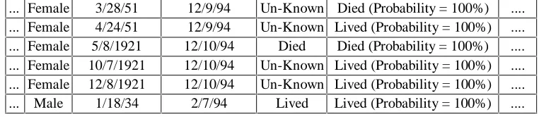
We used Easy Miner to classify records of patients that had heart attack based on the values of attribute Lived. By using a relatively small training set, we built a classifier for attribute Lived and after that we used that classifier to classify all the records in the medical database. A part of the results of the classification process is shown in Figure 2. The attribute Predicted Lived contains the prediction/classification for attribute Lived.

… ..

Sex Date of Birth Date of Stroke Lived Predicted Lived …..

… ..

Male 9/26/1925 11/13/94 Lived Lived (Probability = 100%) ….. ...

.

Male 9/21/1924 9/23/94 Died Died (Probability = 100%) .... ...

.

Male 11/1/1921 9/23/94 Un-Known Lived (Probability = 100%) .... ...

.

Male 10/7/1921 9/23/94 Un-Known Died (Probability = 100%) .... ...

.

... .

Female 3/28/51 12/9/94 Un-Known Died (Probability = 100%) .... ...

.

Female 4/24/51 12/9/94 Un-Known Lived (Probability = 100%) .... ...

.

Female 5/8/1921 12/10/94 Died Died (Probability = 100%) .... ...

.

Female 10/7/1921 12/10/94 Un-Known Lived (Probability = 100%) .... ...

.

Female 12/8/1921 12/10/94 Un-Known Lived (Probability = 100%) .... ...

.

[image:9.612.102.483.73.156.2]

Male 1/18/34 2/7/94 Lived Lived (Probability = 100%) ....

Figure 2: Classified Medical Data

3

Association Rules

With the wide applications of computers and automated data collection tools in business transactions processing, massive amounts of transaction data have been collected and stored in databases. Discovery of interesting association or sequential patterns among those huge amounts of data is an area in which the recent research of data mining is focused. Association rules describe how often two facts happen together. For instance some association rules that could exist in a supermarket database are: “most customers with children buy a particular brand of cereal if it includes baseball cards”, “most customers who buy beer, buy also chips”.

3.2 Definition and properties of Association Rules

An association rule is a rule, which implies certain association relationships among a set of objects in a database. The formal definition of such kind of rules is the following[7].

Let I={i1, i2,...,im} be a set of items. Let DB be a database of transactions, where each

transaction T consists of a set of items such that

T

⊆

I

. Given an itemset

X

⊆

I

, a transaction T contains X only and only if X ⊆T. An association rule is an implication of the form X ⇒Y, where X ⊆ I, Y⊆Iand X∩ = ∅Y . The association rule X ⇒Y holds in DB with confidence

c if the probability of a transaction in DB which contains X also contains Y is c. The association

rule X ⇒Y has support s in DB if the probability of a transaction in DB contains both X and Y is s. The task of mining association rules is to find all the association rules whose support is larger than a minimum support threshold _l′and whose confidence is larger than a minimum

confidence threshold _l′.

3.3 A method for Mining Association Rules

When we examined classification, we saw that a decision tree classifier is a collection of

IF-THEN rules that are expressed by its individual paths. This is a semantic characteristic of

decision trees and we are taking advantage of it in order to develop a method for finding association rules from a database. The rules that our method discovers have the form: X⇒Y, where X is a set of conditions upon the values of several attributes and Y a specific value of one attribute. This attribute Y is called interesting attribute.

The method that we are going to discuss has three simple steps: 1. Data Preparation

3.3.1 Data Preparation

In this stage, the data set in which there is interest on finding association rules, is prepared for applying the method that is going to be presented. In order to do that, and convert the examined data set into our method required format, the next steps must be followed.

1. The interesting attribute, in which there is interest on finding association rules, must be selected and discriminated from the others. In case that there is interest on more than one attribute, then the interesting attribute can be constructed from the join of these attributes.

2. Generalisation induction is performed on the interesting attribute by using, the relative with that attribute, concept hierarchies. In case that the interesting attribute is of numeric type, then its values are being separated into a number of ranges. Then each value of the numeric attribute is replaced by the range that it belongs. So, by this method the initially numeric attribute has been converted into a categorical one with only a few values of higher level. Another result of the generalisation induction on the interesting attribute, is that the discovered rules X ⇒ Y will have higher confidence because Y will have also higher support.

3. If among the data set there are categorical attributes (except the interesting one) that have a large number of distinct values, then the attribute-oriented induction should be performed on them as well. This results in viewing the data in abstractions that are more useful and in generating candidate data sets for finding association rules, that have quite significant support.

3.3.2 Generation of Rules

After the stage of preparation of data, the interesting attribute can be considered as the class label of the whole set of data. Hence, a decision tree classifier can be constructed, based on that classifying attribute. Each path of this decision tree represents one or more rules of the form:

IF (sequence of intermediate conditions) THEN (classifying attribute value)

The confidence of each generated rule from such a path is rj /r, where rj is the number of tuples of each class j that has records in the data set of that leaf, and r is the total number of the records of that data set.

3.3.3 Selection of Strong Rules

After extracting all the rules from the built decision tree, we select only those that are strong. As strong rules have been defined the rules A⇒B that the support of A and B are above the minimum support threshold, and their confidence is greater than the minimum confidence threshold.

In the following table there rules that were discovered by using this technique of Easy Miner are presented. These rules concern the Credit database.

Rule’s Body Support Confidence

IF ( (Marital_Status IN {Single}) ) THEN (Home = Rent) 16.22% 65.15% IF ( (Marital_Status NOT_IN {Single}) (Account_Status IN {60 days late}) (1 <

Nbr_Children) (Savings_Account IN {Yes}) (1187< Mo_Income) ) THEN (Home = Own)

IF ( (Marital_Status NOT_IN {Single}) (Account_Status IN {Balanced}) (1611.50 < Mo_Income <= 2918.50) (Checking_Account IN {No}) ) THEN (Home = Own)

14.99% 100.00%

IF ( (Marital_Status NOT_IN {Single}) (Account_Status IN {Balanced}) (3047.50 < Mo_Income <= 3633) (Nbr_Children < 3) ) THEN (Home = Own)

10.57% 100.00%

IF ( (Marital_Status NOT_IN {Single}) (Account_Status IN {Balanced}) (3633.50 < Mo_Income) (Nbr_Children < 3) ) THEN (Home = Own)

10.57% 93.02%

Summary

In this paper, our approaches for the discovery of patterns in time-oriented data are introduced. We also presented Easy Miner, our mining tool designed and developed at UMIST. Major components of Easy Miner including association rules, classification rules and relevance analysis are described in details with examples.

We think the first consideration for constructing an effective pattern discovery system should be given to testing the appropriateness and applicability of the framework. We have started in this direction by experimenting with a large stroke and quality of hypertension control dataset.

In summary, the work reported in this paper focuses on two areas and their integration. On one side, data mining as a technique for discovery of interesting patterns from database and on the other side time-oriented data as a rich and valuable source of data. We believe that their integration will lead to even higher quality data and discovered patterns.

REFERENCES

[1] Fayyad UM, Piatetsky-Shapiro, Smyth P., Uthurusamy R. Advances in Knowledge Discovery and Data Mining. AAAI/MIT Press, 1995.

[2] Agrawal R., Imienlinski T., Swami A., "Database Mining: A Performance Perspective", IEEE Trans. on Knowledge and Data Engineering Dec. 1993, vol. 5 no. 6, pp. 914--925.

[3] Agrawal R, Srikant R. Mining Sequential Patterns. In Proceedings of Eleventh International Conf. on Data Engineering, March 1995, Taipie, Taiwan, pp. 3-14.

[4] Frawley J, Piatetsky-Shapiro G, Matheus C. J. Knowledge Discovery in Databases: An Overview, in Knowledge Discovery in Databases. Cambridge, MA: AAAI/MIT, 1991, pp. 1-27.

[5] Kamber M, Winstone L., Gong W., Cheng S., and Han J. Generalisation and Decision Tree Induction: Efficient Classification in Data Mining. In Proc. of 1997 Int’l Workshop on Research

Issues on Data Engineering (RIDE’97) , pages. 111-120, Birmingham, England, April 1997.

[6] Mehta M., Agrawal R. , and Rissanen J. SLIQ: A Fast Scalable Classifier for Data Mining. In Proc. of the Fifth Int’l Conference on Extending Database Technology (EDBT), Avignon, France, March 1996.

[7] Shafer J., Mehta M., Agrawal R. SPRINT: A Scalable Classifier for Data Mining. In Proc.