DEVELOPMENT OF A NEW COMPUTATIONAL
MODEL FOR MAPPING, LEARNING AND MINING
OF 3D SPATIO-TEMPORAL fMRI DATA
NORHANIFAH BINTI MURLI
A Thesis submitted to Auckland University of Technology in fulfilment of the requirements for the degree of
Doctor of Philosophy (PhD)
2015
Knowledge Engineering and Discovery Research Institute Faculty of Design and Creative Technologies
ii CONTENTS
ACKNOWLEDGEMENTS ... XVIII
ABSTRACT ... XX
CHAPTER 1 ... 1
INTRODUCTION ... 1
1.1 BACKGROUND ... 1
1.2 MOTIVATION ... 2
1.3 RESEARCHOBJECTIVES ... 4
1.4 SPECIFICRESEARCHQUESTIONS ... 4
1.5 THESISSTRUCTURE ... 5
1.6 THESISCONTRIBUTION ... 6
1.7 PUBLICATION ... 8
1.8 CHAPTERSUMMARY ... 8
CHAPTER 2 ... 9
REVIEWOFSPIKINGNEURALNETWORKS ... 9
2.1 INTRODUCTIONTOSPIKINGNEURALNETWORKS ... 9
2.2 DATAENCODINGMETHODS ... 11
2.2.1 Rate Code ... 12
2.2.2 Pulse Code ... 13
2.3 NEURONMODEL ... 15
2.3.1 Hodgkin-Huxley Model (HHM) ... 15
2.3.2 Leaky Integrate-and-Fire Model (LIFM) ... 16
2.3.3 Izhikevich Model (IM) ... 17
2.3.4 Spike Response Mode (SRM) ... 18
2.3.5 Thorpe Model (TM) ... 18
2.3.6 Probabilistic Spiking Neuron Model (pSNM) ... 19
2.4 LEARNING ... 20
2.4.1 SpikeProp ... 20
2.4.2 One-Pass Algorithm ... 21
2.4.3 Spike-Time Dependent Plasticity (STDP) ... 21
2.4.4 Spike-Driven Synaptic Plasticity (SDSP)... 22
2.5 LIQUIDSTATEMACHINE ... 23
2.6 APPLICATIONOFSNNANDTOOLS ... 24
2.6.1 SNN Applications with Supervised Learning Paradigm ... 24
2.6.2 Applications Using Unsupervised Learning Paradigm ... 25
2.6.3 SNN Tools ... 25
iii
CHAPTER 3 ... 27
REVIEWOFTHENEUCUBEARCHITECTURE ... 27
3.1 LOWESTLEVEL:THEINPUTMODULE ... 28
3.1.1 Population Rank Coding ... 28
3.1.2 AER Data Encoding ... 29
3.2 MIDDLELEVEL:THENEUCUBEMODULE ... 29
3.2.1 The NeuCube Structure ... 29
3.2.2 The Neuron Model ... 32
3.2.3 The Learning Rule ... 33
3.2.4 The Evolvability of the NeuCube ... 34
3.3 HIGHESTLEVEL:THEOUTPUTMODULE ... 34
3.3.1 Dynamic Evolving Spiking Neural Networks (deSNN) ... 35
3.4 NEUCUBEBSTRUCTUREFORSPATIO-TEMPORALMODELLINGANDPATTERN RECOGNITIONOFBRAINSIGNALS ... 37
3.4.1 Spatio-Temporal Brain Data (STBD) and Spatio-Temporal Pattern Recognition (STPR) ... 37
3.4.2 The NeuCubeB Template ... 38
3.5 CHAPTERSUMMARY ... 38
CHAPTER 4 ... 40
REVIEWOFFUNCTIONALMAGNETICRESONANCEIMAGING(FMRI) ... 40
4.1 INTRODUCTIONTOIMAGINGTECHNIQUES ... 40
4.2 FUNCTIONALMAGNETICRESONANCEIMAGING(FMRI) ... 41
4.3 EXISTINGMETHODSFOR FMRIDATAANALYSIS ... 43
4.4 SELECTINGFEATURESOF FMRIDATA ... 45
4.5 CHAPTERSUMMARY ... 46
CHAPTER 5 ... 48
REVIEWOFEXISTINGTECHNIQUESTOSTARPLUS FMRIDATA ... 48
5.1 ABOUTSTARPLUSDATA ... 48
5.2 EXPERIMENTSETTING ... 50
5.3 EXPERIMENTRESULT ... 53
5.4 CHAPTERSUMMARY ... 55
CHAPTER 6 ... 57
NEUCUBEBASEDMETHODOLOGYFOR FMRIDATAMODELLING ... 57
6.1 INDIVIDUALINPUTNEURONMAPPING ... 58
6.2 MAPPINGILLUSTRATIONOFINDIVIDUALNEURONASINPUTNEURON ... 60
6.3 MAPPINGILLUSTRATIONOFNEURONCLUSTERASINPUT ... 61
6.4 VISUALIZATION ... 62
iv
6.5 CHAPTERSUMMARY ... 67
CHAPTER 7 ... 69
CASESTUDY1:APPLICATIONOFNEUCUBEBONSTARPLUSDATA ... 69
7.1 EXPERIMENTALSETUP ... 69
7.2 MAPPINGOF3DSTARPLUS FMRIDATAINTONEUCUBEB ... 69
7.2.1 Neuron Mapping for Each Subjects... 70
7.3 DATAENCODING ... 91
7.4 DATALEARNING ... 92
7.5 MININGUSINGDYNAMICEVOLVINGSPIKINGNEURALNETWORKS(DESNN) ... 94
7.6 RESULTANDDISCUSSION ... 96
7.6.1 Classification Results ... 96
7.7 NEURONSCONNECTIVITY ... 99
7.7.1 NeuCubeB Visualization for Spatio-temporal Connections Based on the fMRI Spiking Activity for Sentence Stimulus ... 99
7.7.2 NeuCubeB Visualization for Spatio-temporal Connections Based on the fMRI Spiking Activity for Picture Stimulus ... 100
7.8 CHAPTERSUMMARY ... 103
CHAPTER 8 ... 105
CASESTUDY2:APPLICATIONOFNEUCUBEBMETHODOLOGYONHAXBYVISUAL OBJECTRECOGNITIONDATA ... 105
8.1 EXPERIMENTALSETUP ... 105
8.2 MAPPINGOFNIFTI-1 FMRIDATAINTONEUCUBEB ... 109
8.2.1 Neuron Mapping ... 110
8.3 DATAENCODING ... 114
8.4 DATALEARNING ... 115
8.4.1 Stimulus by Stimulus Learning for Each Subject Approach ... 115
8.4.2 Subject by Subject (Personalized) Approach ... 117
8.5 MININGUSINGDYNAMICEVOLVINGSPIKINGNEURALNETWORKS(DESNN) . 118 8.6 RESULTANDDISCUSSION ... 118
8.6.1 Stimulus by Stimulus for Each Subject Classification Results ... 118
8.6.2 Subject by Subject (Personalized) Classification Result ... 122
8.7 NEURONSCONNECTIVITY ... 125
8.7.1 NeuCubeB Visualization for Spatio-temporal Connections Based on the fMRI Spiking Activity for Face Stimulus ... 125
8.7.2 NeuCubeB Visualization for Spatio-temporal Connections Based on the fMRI Spiking Activity for Scrambled Picture Stimulus ... 129
v
CHAPTER 9 ... 134
CONCLUSIONANDFUTUREDIRECTION ... 134
9.1 CONCLUSION ... 134
9.2 THESISCONTRIBUTIONS ... 134
9.3 FUTUREDIRECTION ... 138
9.3.1 Parameters Optimization ... 138
9.3.2 Automatic Voxel Mapping ... 139
9.3.3 Specialized SNN Hardware Implementation ... 139
10REFERENCES ... 140
11APPENDIX A STARPLUS MAIN SOURCE CODES ... 155
vii LIST OF FIGURES
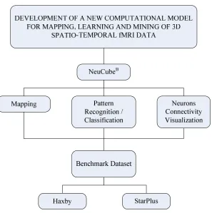
Figure 1-1 : A visual summary of contributions of the thesis in terms of data
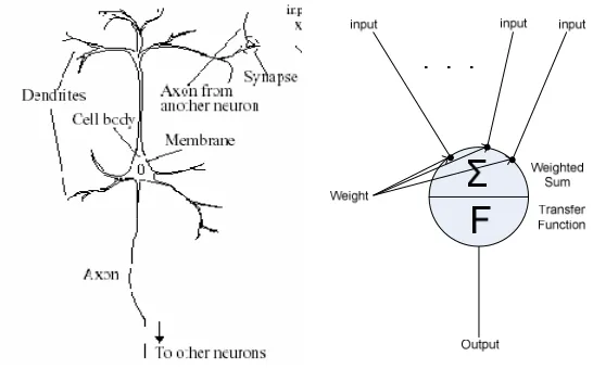
mapping, classification and connectivity visualization. ...7 Figure 2-1: Biological neuron (Hemming, 2003)(left) and artificial neuron model
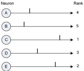
(right) ... 10 Figure 2-2: Ranking of spikes in a population of neurons applied in ROC method .. 14 Figure 2-3: Illustration of population rank order coding (Abdul Hamed, 2012;
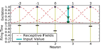
Schliebs, Defoin-Platel, & Kasabov, 2009) ... 15 Figure 2-4: Simplified representation of pSNM with all probabilistic parameters
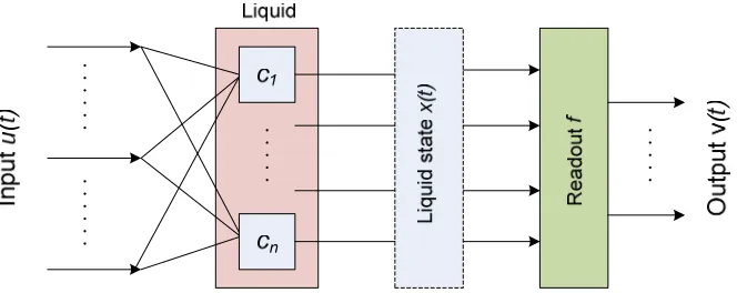
and one synaptic connection ... 19 Figure 2-5: The LSM architecture consists of three main layers: input neuron
layer, liquid state layer and readout function layer. ... 23 Figure 3-1: General architecture of NeuCube that consists of four integrated
modules: Input, NeuCube, GRN and Output module ... 28 Figure 3-2: The Talairach Daemon Software for brain areas visualization.
(http://www.talairach.org/applet/) ... 30 Figure 3-3: The Talairach atlas with lobe labels (illustrated with patterned colour
fills), gyral structures (illustrated with bold colour outlines), and several Brodmann areas (illustrated with solid colour fills) (Lancaster et al., 2000). ... 30 Figure 3-4: (a) Schematic representation of LIFM of a spiking neuron and (b)
Functionality of LIFM in which the red line represents the membrane potential, the middle row represents the output spikes and on top is the input train of spikes. ... 32 Figure 3-5: Approximate mapping of 1,471 NeuCube neurons displayed in dark
blue dots. The cyan and yellow dots are the fMRI input data before initialization (left) and after initialization (right) respectively. ... 38 Figure 4-1: Brain images in vertical and horizontal slice: in sagittal, coronal and
axial views (left). Slices of brain taken over time i.e. 32 images for a volume of brain (images are viewed using FSLView (FSLView,
2012) software (right). ... 42 Figure 4-2: Surface renderings of 3D brain images. Small voxels (left, with 1
viii Figure 5-1: 25 anatomically defined region of interest in human brain used in the
study ... 50 Figure 5-2: 50 most significant features are selected using SNR data analysis for
CALC region. ... 52 Figure 5-3: 100 most significant features are selected using SNR data analysis for
CALC region ... 52 Figure 5-4: Percentage of classification accuracy for 50 features selected based on
SNR ... 53 Figure 5-5: Percentage of classification accuracy for 100 features selected based
on SNR ... 54 Figure 6-1: Schematic diagram of NeuCubeB architecture involving mapping,
learning and mining phases ... 58 Figure 6-2: Determination of value that will be used in mapping
of into of NeuCubeB. ... 60
Figure 6-3: NeuCubeB 50 and the neighbouring 6 fMRI voxel coordinates that are within 7 mm radius. ... 61 Figure 6-4: NeuCubeB 500, 1009 and 1105 with their neighbouring fMRI neurons
viewed from direction. ... 62 Figure 6-5: NeuCubeB neurons (black dots) and fMRI input neurons (blue
crosses) mapped and visualized together in 3D view in initialization stage. ... 63 Figure 6-6: NeuCubeB neurons (black dots) and fMRI neurons (blue crosses) in
three views (in , and views) ... 64 Figure 6-7: NeuCubeB (cyan squares) and fMRI (blue squares) input neurons
mapping, in each −slice, in which each sub-figure represent a single slice. ... 65 Figure 6-8: Visualization of neurons connectivity for fMRI data stimulus before
(top) and after (down) STDP learning in 3D view. Positive
connections are in blue and negative connections are in red. ... 67 Figure 7-1: Mapping of 4,949 fMRI neurons (blue crosses) into NeuCubeB input
neurons (black dots) for subject S04799 in 3D view. ... 71 Figure 7-2: NeuCubeB and segmented StarPlus fMRI neurons for subject S04799.
ix Figure 7-3: NeuCubeB neurons (black dots) and fMRI S04799 input neurons (blue
dots) in three views (in , and views). ... 73 Figure 7-4: NeuCubeB neurons (cyan squares) and fMRI S04799 input neurons
(blue dots) mapping, in each 11 −slice, in which each sub-figure represents a single slice. ... 74 Figure 7-5: Mapping of 5,015 fMRI neurons (blue crosses) into NeuCubeB input
neurons (black dots) for subject S04820 in 3D view. ... 74 Figure 7-6: NeuCubeB and segmented StarPlus fMRI neurons for subject S04820.
Different colours represent different brain areas. ... 75 Figure 7-7: NeuCubeB neurons (black dots) and fMRI S04820 input neurons (blue
dots) in three views (in , and views). ... 76 Figure 7-8: NeuCubeB neurons (cyan squares) and fMRI S04820 input neurons
(blue dots) mapping, in each 11 −slice, in which each sub-figure represents a single slice. ... 77 Figure 7-9: Mapping of 4,698 fMRI neurons (blue crosses) into NeuCubeB input
neurons (black dots) for subject S04847 in 3D view. ... 77 Figure 7-10: NeuCubeB and segmented StarPlus fMRI neurons for subject S04847.
Different colours represent different brain areas. ... 78 Figure 7-11: NeuCubeB neurons (black dots) and fMRI S04847 input neurons (blue
dots) in three views (in , and views). ... 79 Figure 7-12: NeuCubeB neurons (cyan squares) and fMRI S04847 input neurons
(blue dots) mapping, in each 11 −slice, in which each sub-figure represents a single slice. ... 80 Figure 7-13: Mapping of 5,135 fMRI neurons (blue crosses) into NeuCubeB input
neurons (black dots) for subject S05675 in 3D view. ... 80 Figure 7-14: NeuCubeB and segmented StarPlus fMRI neurons for subject S05675.
Different colours represent different brain areas. ... 81 Figure 7-15: NeuCubeB neurons (black dots) and fMRI S05675 neurons (blue dots)
in three views (in , and views). ... 82 Figure 7-16: NeuCubeB neurons (cyan squares) and fMRI S05675 input neurons
x Figure 7-17: Mapping of 5,062 fMRI neurons (blue crosses) into NeuCubeB input
neurons (black dots) for subject S05680 in 3D view. ... 83 Figure 7-18: NeuCubeB and segmented StarPlus fMRI neurons for subject S05680.
Different colours represent different brain areas. ... 84 Figure 7-19: NeuCubeB neurons (black dots) and fMRI S05680 neurons (blue dots)
in three views (in , and views). ... 85 Figure 7-20: NeuCubeB neurons (cyan squares) and fMRI S05680 input neurons
(blue dots) mapping, in each 11 −slice, in which each sub-figure represents a single slice. ... 86 Figure 7-21: Mapping of 4,634 fMRI neurons (blue crosses) into NeuCubeB
neurons (black dots) for subject S05710 in 3D view. ... 86 Figure 7-22: NeuCubeB and segmented StarPlus fMRI neurons for subject S05710.
Different colours represent different brain areas. ... 87 Figure 7-23: NeuCubeB neurons (black dots) and fMRI S05710 input neurons (blue
dots) in three views (in , and views). ... 88 Figure 7-24: NeuCubeB neurons (cyan squares) and fMRI S05710 input neurons
(blue dots) mapping, in each 11 −slice, in which each sub-figure represents a single slice. ... 89 Figure 7-25: NeuCubeB and StarPlus 7 ROIs neurons mapping in view.
Different colour represents different ROI. Black dots are NeuCubeB
coordinates and blue crosses are the other StarPlus neurons. ... 90 Figure 7-26: NeuCubeB and StarPlus 25 ROIs neurons mapping in 2D view. ... 90 Figure 7-27: NeuCubeB and segmented StarPlus 25 ROIs neurons mapping in 3D
view. ... 91 Figure 7-28: Neuron connections after initialization (left) and neuron connections
after unsupervised learning (right). ... 94 Figure 7-29: Data design for: (a) NeuCubeB model. Brain volumes within the
same trial are learned as one spatio-temporal pattern i.e. one sample and propagated one after another. (b) Standard classifiers model. Brain volumes within the same trial are concatenated and taken as a single sample. ... 95 Figure 7-30: A snapshot of a software implementation of the NeuCubeB
xi The classification model used is deSNN an accuracy of 100% for
Class 1 and 80% for Class 2 ... 97 Figure 7-31: Visualization of fMRI data model and connectivity between neurons
of eSNN: (a) no spiking activity yet, inactive neurons are in blue, fMRI data neurons (input neurons) are in yellow; (b) spiking activity: active neurons are represented in red, inactive neurons are represented in blue, positive input neurons are represented in magenta, negative input neurons are represented in cyan and zero input are represented in yellow; (c) neurons connectivity before training (small world connection), positive connections are in blue and negative
connections in red; (d) neurons connectivity after training. ... 98 Figure 7-32: Visualization of neurons connectivity for data Sentence stimulus after
initialization in 3D view. For visualization purposes, displayed connections are based on weight more than 0.19 (left) and weight more than 0.09 (right). ... 101 Figure 7-33: Visualization of neurons connectivity for data Sentence stimulus after
STDP learning in 3D. For visualization purposes, displayed connections are based on weight more than 0.19 (left) and weight more than 0.09 (right). ... 101 Figure 7-34: Visualization of neurons connectivity for data Picture stimulus after
initialization in 3D view. For visualization purposes, displayed connections are based on weight more than 0.19 (left) and weight more than 0.09 (right). ... 102 Figure 7-35: Visualization of neurons connectivity for data Picture stimulus after
STDP learning in 3D view. For visualization purposes, displayed connections are based on weight more than 0.19 (left) and weight more than 0.09 (right). ... 102 Figure 8-1: Examples of stimulus used in the Haxby visual experiment. Subjects
performed a one-back repetition detection task i.e. the same object is presented with different views. Picture is taken from Haxby et al., (2001). ... 107 Figure 8-2: Illustration of Haxby data (Haxby et al., 2011) for SUB001 when the
subject is presented with Face stimulus for ID=1 and Run=1 ... 109 Figure 8-3: Visualization of coordinates that are mapped into the NeuCubeB.
Cyan dots represent the coordinates of Haxby fMRI brain data while blue dots are coordinates of NeuCubeB, in 3D view for subject
SUB001. ... 111 Figure 8-4: Visualization of coordinates that are mapped into the NeuCubeB.
xii while blue dots are coordinates of NeuCubeB, in view for subject
SUB001. ... 111 Figure 8-5: Visualization of coordinates that are mapped into the NeuCubeB.
Cyan dots represent the original voxels of Haxby fMRI brain data while blue dots are coordinates of NeuCubeB, in view for subject SUB001. ... 112 Figure 8-6: Visualization of coordinates that are mapped into the NeuCubeB.
Cyan dots represent the original voxels of Haxby fMRI brain data while blue dots are coordinates of NeuCubeB, in view for subject
SUB001. ... 112 Figure 8-7: Visualization of mapped Haxby coordinates into NeuCubeB
coordinates, in view for subject SUB001 after the mapping
procedure. ... 113 Figure 8-8: Visualization of mapped Haxby coordinates into NeuCubeB
coordinates, in view for subject SUB001 after the mapping
procedure. ... 113 Figure 8-9: Visualization of mapped Haxby coordinates into NeuCubeB
coordinates, in view for subject SUB001 after the mapping
procedure. ... 114 Figure 8-10: Neuron connections after initialization (left) and neuron connections
after unsupervised learning (right). ... 117 Figure 8-11: A snapshot of a software implementation of the NeuCubeB
architecture for classification of 2 class fMRI data for SUB004. The parameter values are as stated in section 7.5.2. The classification model used is deSNN with an accuracy of 83.3% for Class 1 and
83.3% for Class 2. ... 120 Figure 8-12: Visualization of fMRI data model and connectivity between neurons
of eSNN: (a) no spiking activity yet, inactive neurons are in blue, fMRI data neurons (input neurons) are in yellow; (b) spiking activity: active neurons are represented in red, inactive neurons are represented in blue, positive input neurons are represented in magenta, negative input neurons are represented in cyan and zero input are represented in yellow; (c) neurons connectivity before training (small world connection), positive connections are in blue and negative connection in red; (d) neurons connectivity after training. ... 121 Figure 8-13: A snapshot of a software implementation of the NeuCubeB
xiii Figure 8-14: Visualization of fMRI data model and connectivity between neurons
of eSNN for SUB001 for Face Versus Not Face test run: (a) no spiking activity yet, inactive neurons are in blue, fMRI data neurons (input neurons) are in yellow; (b) spiking activity: active neurons are represented in red, inactive neurons are represented in blue, positive input neurons are represented in magenta, negative input neurons are represented in cyan and zero input are represented in yellow; (c) neurons connectivity before training (small world connection), positive connections are in blue and negative connection in red; (d) neurons connectivity after training. ... 124 Figure 8-15: Visualization of neurons connectivity for Face stimulus (a) before and
(c) after STDP learning with (b) weight>=0.09 and (d) weight>=0.19. Positive connections are in blue and negative connections are in red. . 127 Figure 8-16: Approximated location of densely interconnected neurons that are
activated when seeing Face stimulus before training. ... 127 Figure 8-17: Approximated location of densely interconnected neurons that are
activated when seeing Face after the learning process. More connections are created in areas SFG, MFG, IFG, STG, IFG, SPL, IPL and OL. ... 128 Figure 8-18: Visualization of neurons connectivity for Face stimulus when weight
is greater than 0.21 in 3D view (left) and in view (right). ... 128 Figure 8-19: Visualization of neurons connectivity for Scrambled Picture stimulus
(a) before and (c) after STDP learning with (b) weight>=0.09 and (d) weight>=0.19. Positive connections are in blue and negative
connections are in red. ... 130 Figure 8-20: Approximated location of densely interconnected neurons before
training. ... 131 Figure 8-21: Approximated location of densely interconnected neurons after
training. More connections are created in areas SFG, MFG, IFG, STG, IFG, SPL, IPL and OL. ... 131 Figure 8-22: Visualization of neurons connectivity for Scrambled Picture stimulus
xiv LIST OF TABLES
Table 3-1: deSNN training algorithm ... 36 Table 5-1: Experiment Conditions ... 49 Table 5-2: ROIs considered in the classification task and the number of features
in each region for subject S04820 ... 50 Table 5-3: Classification accuracy percentage for each region using SVM and
MLP classifiers (A=SVM classifier, B=MLP classifier) ... 53 Table 7-1: Voxel details for each subject ... 71 Table 7-2: Brain region representation ... 72 Table 7-3: Total number of neurons for each subject, the actual input neurons
and the corresponding spike states for training and validation ... 92 Table 7-4: Classification results between classical machine learning and
NeuCubeB. The dataset consists of 20 samples of 1,471 pixel value variables ... 97 Table 8-1: Example of task run 1 for SUB001 in which the subject is presented
first with Scissors, followed by Face, Cat, Shoe, House, Scrambled Picture, Bottle and finally Chair stimulus, and the brain image is captured in every 2.5 seconds (0.5 seconds to display stimulus and another 1.5 seconds are the interval between stimuli) ... 108 Table 8-2: Total number of neurons for each subject, the actual input neurons
and the corresponding spike states for training and validation for a stimulus against the other stimulus ... 115 Table 8-3: Total number of neurons for each subject, the actual input neurons
and the corresponding spike states for training and validation for a stimulus against the other 7 stimuli ... 115 Table 8-4: Classification accuracy percentage of Class1 (Face) and Class 2
(Scrambled Pictures) stimulus for all subjects ... 120 Table 8-5: Overall percentage of classification results for each subject for Face
versus Not Face and Scrambled Pictures versus Not Scrambled
xv LIST OF ABBREVIATIONS
3D three dimensional
AER Address Event Representation ANNs Artificial Neural Networks BCI Brain Computer Interface BD Bilateral Dorsolateral
BOLD Blood Oxygen Level Dependent
BSA Ben’s Spike Algorithm
CALC Calcarine Sulcus
CMU Carnegie Mellon University CPU Central Processing Unit
CT Computed Tomography
deSNN Dynamic Evolving Spiking Neural Networks DICOM Digital Imaging and Communications in Medicine DTI Diffusion Tensor Imaging
ECoS Evolving Connectionist System
EEG Electroencephalography
ESNN Evolving Spiking Neural Networks FEF Frontal Eye Field
FIR Finite Impulse Response
FMRI functional Magnetic Resonance Imaging GENESIS General Neural Simulation System
GRN Gene Regulatory Networks
GSC Generalized Sparse Classifier
HHM Hodgkin-Huxley Model
IFG Inferior Frontal Gyrus
IM Izhikevich Model
IPL Inferior Parietal Lobule IPS Intraparietal Sulcus
ITG Inferior Temporal Gyrus
ITL Inferior Temporal Lobule LIFM Leaky Integrate-and-Fire Model
xvi
LTP Long Term Potential
LSM Liquid State Machine
MEG Magneto Encephalography
MFG Medial Frontal Gyrus
MLP Multilayer Perceptron
MLR Multiple Linear Regression MNI Montreal Neurological Institute MRI Magnetic Resonance Imaging NEST Neural Simulation Tool NIRS Near Infrared Spectroscopy
OL Occipital Lobe
OPER Opercularis
PET Positron Emission Tomography PPREC Posterior Precentral Sulcus
pSNM Probabilistic Spiking Neuron Model pSNN probabilistic Spiking Neural Networks POC Population Rank Order Coding
PROC Population Rank Order Coding PSO Particle Swarm Optimization PSP Postsynaptic Potential
PSTH Peri-Stimulus-Time Histogram
RO Rank Order
ROC Rank Order Coding
ROI Region of Interest
SDSP Spike-Driven Synaptic Plasticity SFG Superior Frontal Gyrus
SMA Supplementary Motor Area
SNN Spiking Neural Networks
SNR Signal to Noise
SMG Supramarginal Gyrus
SPAN Spike Pattern Association Neuron SpikeNET Spike Network
SPL Superior Parietal Lobe
SPM Statistical Parametric Mapping
xvii SSTD Spatio- Spectro Temporal Data
STBD spatio- and spectro-temporal brain data STDP Spike Timing Dependent Plasticity
STG Superior Temporal Gyrus
STP Spatio-temporal Pattern
STPR Spike Time Pattern Recognition
SWC Small World Connections
SVM Support Vector Machine
TL Temporal Lobe
TM Thorpe Model
TR Time of Repetition
xviii
ACKNOWLEDGEMENTS
I would like to extend my gratitude and to acknowledge some of the many individuals who have educated, inspired, motivated and supported me towards the completion of this PhD study.
My sincerest and highest appreciation to my primary supervisor, Professor Ni-kola Kasabov, who offered me the opportunity to be in his dedicated PhD supervision and gave me the chance to be one of the family members’ to the prominent Knowledge Engineering and Discovery Research Institute (KEDRI). Your intellectual supports, great ideas, comments, and encouragement were very significant for me in ensuring this study persisted in the right path. It was you who have motivated and inspired me to continue with the study and not giving up during the fuzzy and blurry duration of my study years. Thank you so much for your patience, tolerance and confidence.
Special thanks to my secondary supervisor, Dr. Russel Pears who introduced me to the machine learning and computational intelligence field, and for allowing me to at-tend his class on Data Mining and Knowledge Discovery. My acknowledgment is also to Dr. Bana Handaga for his continuous help and support. He has constantly spent countless hours to teach me programming and to help in my paper writings.
I had a great time learning and working in KEDRI which provided a multiracial and exciting research environment where we could exchange knowledge and ideas, and once in a while to have party just to release the pressure and tension. To Joyce D’Mello, the manager of KEDRI who has very beautiful eyes, you will always be re-membered for your kindness, encouragement and thoughtfulness especially during my hard times. My life would be difficult and miserable if it wasn’t with your help. Thank you heaps!
xix advice. My gratitude also to my UTHM-PGR4 girlfriends: Hannani Aman, Norlida Hassan, Isredza Rahmi A. Hamid, Nurul Aswa, Mahfuzoh Wasikon, Yana Mazwin Hassim and Nor Yusliza Abdullah for your continuous supports and motivation.
I would like also to thank the Malaysian Ministry of Higher Education and Uni-versiti Tun Hussein Onn Malaysia for providing the scholarship during the entire phase of my study, and Auckland University of Technology, specifically KEDRI, for provid-ing good research environment and state of the art facilities.
xx
ABSTRACT
The application of data mining techniques, particularly classification of spatio-temporal 3D functional magnetic resonance images has received growing attention in the litera-ture. Spatio or spatial component as well as temporal component are factors of high importance in determining and recognizing brain state in response to external stimuli. Structural and functional brain data have been hugely collected, in an attempt to im-prove brain cognitive abilities and processing capabilities, as well as advancement in medicine, health, education, Brain Computer Interface and games. A particular spatio- and spectro-temporal brain data (STBD), functional Magnetic Resonance Imaging (fMRI), provides a comprehensive detail of brain activation when a certain stimulus is presented to the subject resulting from the changes of oxygen level in the blood vessel of the brain. This oxygen difference between active neurons and inactive neurons is captured in sequence, and the images generated from this (the fMRI) are composed of tens of thousands of individual voxels. These massive voxels are the features to this thesis, which became one of the challenges that had to be faced, in addition to the com-plex format of the data itself.
To some extent, conventional machine learning techniques has successfully process and classify fMRI data. However, these techniques are only best at dealing spa-tial data, which completely neglect the temporal information that this data has.
Thus, this study proposes and presents a novel computational model that specifi-cally process spatial and temporal information of fMRI data, which make use of the newly proposed NeuCube model as its foundation. The derived model, denoted as NeuCubeB utilized the 3D evolving SNN architecture of NeuCube in mapping and learning the data. The model learns from the data; then creates and updates connections between the neurons based on their weights. These connections represent chains of neu-ronal activities which could be reproduced even when only part of the stimuli data is presented, therefore making the NeuCube connections as an associative memory. The model can be used not only to classify brain activation patterns, but also to determine functional trail from the data i.e. to identify brain areas that receive the most activation from the stimulus.
re-xxi searchers, which utilized different types of conventional machine learning techniques. In NeuCubeB, the fMRI features (voxels) are modelled and studied as both spatial and temporal information involving phases of data reading, mapping, and encoding, before they are transferred to initialization and unsupervised learning stage. Connectivity of neurons in the network could be visualized and studied. The visualization can reveal crucial spatio-temporal relationship unseen from the data that are completely ignored by the standard classifiers. For both experiments involving two different sets of fMRI data, NeuCubeB model results in better classification accuracy as compared to the standard classifiers. From this result, it can be concluded that NeuCubeB model is not vulnerable
1
1
Chapter 1
INTRODUCTION
1.1 BACKGROUND
The human brain is the command centre for the complex network of nerves and cells that carry signals to and from the brain to various part of the human body. For instance, when a person looks at a picture, a particular region in the brain will be activated. In order to capture the spatio temporal activation, brain imaging technique, in particular functional magnetic resonance imaging (fMRI) technique, is often used. The technique which detects metabolic activity of brain areas (not neuronal firing itself) is widely available and it allows subjects to be examined noninvasively. More precisely, fMRI measures the blood oxygen level (oxygenated haemoglobin to deoxygenated haemoglo-bin) at many individual locations within the brain. This neural activity is widely be-lieved to influence the level of oxygen in the blood and is known as blood oxygen level dependent (BOLD) response (Mitchell, et. al. 2004).
Images generated from this technique are constructed from two components – spatial/spectral (or spatio) and temporal components. Spatial component is identified as a volume of a brain that can be further sub-divided into smaller three-dimensional (3D) cuboids, known as voxels (volume element). In addition, temporal component is the time acquired scanning the whole volume of a brain. The combination of these spatial and temporal data of the brain images will be the main characteristics to be investigated in this study. Apart from fMRI, electroencephalogram (EEG), diffusion tensor imaging (DTI), magnetoencephalography (MEG) and near-infrared spectroscopy (NIRS) are also known as spatio- and spectro-temporal brain data (STBD). These are largely collected and available for researchers in the field of medicine, health, cognitive sciences, educa-tion and Brain Computer Interface (BCI) to take advantage of.
2 same working principle as STBD in terms of its spiking activity is anticipated to be suitable for the creation of a computational framework for learning and understanding of fMRI as well as other brain data. A newly proposed architecture called NeuCube (Kasabov, 2014) that is based on a 3D evolving SNN (eSNN) is developed to map and learn STBD, thus to better understand the data.
eSNN architecture (Wysoski, Benuskova, & Kasabov, 2006) was inspired by the Evolving Connectionist System (ECoS) (Kasabov, 1998) principles that evolves its structures incrementally in time, i.e. in its neurons and neurons connections. Besides the fact that ECoS could perform training very fast, it is also capable of processing large amount of spatio-temporal data, and it has structures that can accommodate new fea-tures to be added in at a later stage of the learning process. The advantages that ECoS and eSNN have to offer make NeuCube the best architecture to map, train and learn STBD. Previous experiments involving the use of NeuCube in modeling and learning spatio-temporal stroke data (Kasabov et al., 2014) has produced high accuracy in pre-dicting stroke occurrences, thus inspiring more studies to experiment with other variants of STBD.
Undeniably many efforts have been performed to model and process fMRI or other spatio-temporal data but classical machine learning often neglect the temporal component that this data has. We believe that beside the spatial component of fMRI that holds so much information about the brain, the other equally important component i.e. temporal component is also very crucial and very much desired in making accurate decisions.
1.2 MOTIVATION
3 accurate structural and functional brain models (e.g. Izhikevich & Edelman, 2008; Markram, 2006; Toga, Thompson, Mori, Amunts, & Zilles, 2006). However they still could not be used for machine learning and pattern recognition of STBD, which specifi-cally could handle fMRI data modeling and processing that would facilitate researchers to find efficient solutions to important problems such as detecting fMRI cognitive func-tions accurately and interpreting the data model.
Thus there is a significant gap to develop a computational framework that have a generic spatial structure of an approximate map of the human brain in certain coordinate system (e.g. MNI or Talairach); that could also map the spatial location(i.e. voxel coor-dinates) of the incoming brain data; that later on could represent and process the voxels as train of spikes and STBD; and finally that have brain-like learning rules to learn the STBD and evolve when new STBD patterns are presented into the framework. Follow-ing the principle of brain cognitive development, evolvFollow-ing is in terms of learnFollow-ing and recognizing new STBD patterns and adding those patterns into the model. In addition, the framework preserves a spatio-temporal associative memory (i.e. in its neuron con-nections) that can be inferred for new knowledge discovery.
We also believed that the temporal order of fMRI data acquire significant mean-ings to the interpretation and understanding of the brain data. Thus, a framework that can handle this temporal information is very much required i.e. to be able to train the data according to their temporal order, in which the output of the post-synaptic neurons will be greatly influenced by the characteristics of the neurons before them. At the end of the neurons computations, it is hoped that the framework is able to produce more ac-curate results as compared to the temporal-ignorant classifiers that disregard the se-quence of the data.
On top of this, conventional classifiers developed so far are incapable of han-dling large and noisy data, unable to deal with stochastic and dynamic processes while ignoring several equally important parameters required in the computations of spiking neurons (Kasabov, 2010). These variables include the probability of synapses to accept spikes and the emission of neurotransmitters (Lauger, 1995), synaptic scaling, STDP and synaptic redistribution (Abbott & Nelson, 2000), physical properties of neurons’ connections (Huguenard, 2000), new information about neuronal information process-ing in biological neural networks (Gerstner & Kistler, 2002) and gene and protein ex-pression (Kojima & Katsumata, 2008).
4 Because of the complexity of the fMRI data itself (having spatio and temporal informa-tion) together with the fact that it is big in nature (thousands of features but with low number of samples), there are chances that NeuCubeB could provide an environment
that could better process and analyze the fMRI data. The analysis is critical in such a way that it could map the brain data, convert the voxel intensity values into spikes and STBD patterns, learn the STBD patterns, classify and visualize the connections between neurons after the learning process.
1.3 RESEARCH OBJECTIVES
This research has the following objectives:
a. To develop a new methodology for spatio-temporal fMRI data processing
b. To develop a novel fMRI mapping strategy
c. To analyze the neurons connectivity
d. To conduct practical experiments on benchmark datasets
e. To classify the dataset into predefined classes and to compare the findings with performance of other existing well known methods
f. To share research outcomes through presentations and publication of related re-search community
1.4 SPECIFIC RESEARCH QUESTIONS
Aligned with the research objectives, the specific research questions of this study are as follows:
1. How to map the spatial location of the benchmark fMRI dataset into the Neu-CubeB architecture? NeuCubeB (Kasabov, 2014) was predefined as having 1,471
differ-5 ent brain sizes and structures, i.e. mapping of these brains will impose different spatial estimation.
2. Can the learning of large and spatio-temporal fMRI data in the NeuCubeB be better and improved compared to other standard machine learning techniques?
3. What can be learned from the connectivity of neurons in the NeuCubeB before
and after the training? Which part of the brain region will be more activated when a certain stimulus is presented to the subject? Different task will stimulate neurons in different locations to spike, thus more neurons connections will be created.
In brief, this research intends to develop a computational model that could map, learn and mine spatio-temporal brain data specifically fMRI, in which the model is de-veloped, based on the new proposed NeuCubeB architecture. This research also aims to achieve better classification result and better understanding of the fMRI data.
1.5 THESIS STRUCTURE
The thesis is organized in eight chapters and will be explained briefly as the following:
CHAPTER 2 This chapter explains literatures on the backbone and the inspira-tion of the NeuCubeB, which is SNN. Components of SNN that will also be discussed include: models of neurons, available encoding methods that can be used to transform voxels intensity values into spikes and, models of learning. Other related principles that will be introduced in the chapter include eSNN, liquid state machine (LSM) and avail-able SNN tools and applications.
CHAPTER 3 This section starts with an introduction to imaging techniques, followed by reviews in detail of fMRI as one of the imaging techniques that provide im-ages of brain structure in great resolutions, continued with existing methods for fMRI data analysis and finally briefly explains of feature selection.
6 standard classifiers, which are Support Vector Machine (SVM) and Multiple Linear Re-gression (MLR), tested on the dataset is also discussed later in the chapter.
CHAPTER 5 This chapter explains the NeuCube based methodology used in the research. It includes the architecture and principles of the generic NeuCube which include the unsupervised and supervised mode of learning. There will also be reviews on the three levels that define the architecture: the input module (lowest level), the NeuCube module (the middle level) and the output module (the highest level).
CHAPTER 6 The first case study is presented in this chapter which involves the use of StarPlus data as the input to the NeuCubeB. The steps in conducting the ex-periment i.e. data mapping, data encoding, data learning, data classification and result analysis are explained.
CHAPTER 7 Another experiment is carried out using different set of fMRI data which is in a different format from the StarPlus. The same steps are applied to the data, but with different mappings, which represents a new challenge to the research. The rea-son is because of the NII format, which in principal is associated with NIfTI-1 data for-mat. This file type is defined in a 4-dimensional data structure to save the volumetric spatio-temporal fMRI data. The results of the experiment are discussed at the end of the chapter.
CHAPTER 8 This chapter explains the conclusions and future direction of the study.
1.6 THESIS CONTRIBUTION
The following diagram shown in Figure 1-1 summarizes the contributions of this re-search, in terms of the proposed model, datasets used and the problems to be solved. The newly proposed NeuCubeB framework is experimented using two different sets of
7 to their temporal order) into the evolving cube via the input neurons. These spike se-quences are trained using the unsupervised Spike Timing Dependent Plasticity (STDP) learning rule and the temporal relationship between the data are encoded to the connec-tion weights. The spike sequences are then fed into a supervised dynamic evolving Spiking Neural Networks (deSNN) learning rule. An output neuron is created and its connection weights are calculated for the incoming new data (i.e. test data). These gen-erated weights are compared with the weights gengen-erated during the unsupervised learn-ing. In short, the same neurons are spiking to evoke the same temporal connectivity generated during the unsupervised learning (Izhikevich, 2006). Accordingly, in this study, the output neurons learned to classify the spike patterns of fMRI data for both mentioned datasets and this would be the second contribution. And finally, for the third contribution, this study presented spatio-temporal neurons connections based on the fMRI data spiking activity which are displayed using blue line and red line to denote positive spikes and negative spikes respectively.
8
1.7 PUBLICATION
Murli, N., Kasabov, N., &Handaga, B. (2014, January) Classification of fMRI Data in the NeuCubeB Evolving Spiking Neural Network Architecture. In Neural Information Processing (pp. 421-428). Springer International Publishing
Murli, N., Kasabov, N., &Handaga, B. (2015). Evolving Spiking Neural Network for Spatio-temporal Pattern Classification with a Case Study on Visual Object Recognition. Submitted to Journal of Neural Networks.
Kasabov, N., Scott, N, Tu, E., Othman, M., Doborjeh, M., Marks, S., Sengupta, N., Murli, N., Hartono, R., Espinosa-Ramos, I., Capecci, E., Zhou, L., Alvi, F., Wang, G., Taylor, D., Feigin, V., Gulyaev, S., Mahmoud, M., Hou, Z. and Yang, J. (2015). Evolv-ing Spatio-Temporal Data Machines Based on the NeuCube Neuromorphic Framework: Design Methodology and Selected Applications. Submitted to Neural Networks
1.8 CHAPTER SUMMARY
This chapter introduces and describes the study which includes the general view of the problem, the objectives, the motivations for carrying out this study, and the specific re-search questions need to be answered and justified throughout the whole study period. It also reviews the structure of the thesis i.e. the topics that will be covered in the other chapters of the thesis. Thesis contributions and publication are also outlined.
9
2
Chapter 2
REVIEW OF SPIKING NEURAL NETWORKS
This chapter reviews the basis of spiking neural networks (SNN). It will discuss the fundamental components of SNN that includes data encoding methods, neuron models and learning algorithms.
2.1 INTRODUCTION TO SPIKING NEURAL NETWORKS
The human brain is made approximately of 86 billion cells known as neurons (Koch & Reid, 2012) which are connected together in a vast and complex network. These neu-rons are of various types, shapes and functions, and communicate with other neuneu-rons mostly through the generation and propagation of output or action potentials (or better known as spikes). Generally a typical neuron (Figure 2-1) is made of dendrites that act as the collecting points for inputs and propagate them to the cell body/soma. The soma acts as the central processing unit that actually computes all the inputs and makes deci-sion either to generate an output or not. Meanwhile the axon acts as the link to transfer output signals to other neurons. Communicating neurons are linked together through a synapse in which the sending neuron is called as pre-synaptic neuron and the receiving neuron is called as post-synaptic neuron.
10 1961) which is having synchronous inputs and generating real-valued output between 0 and 1, computing the average firing rate of the neuron.
Figure 2-1: Biological neuron (Hemming, 2003) (left) and artificial neuron model (right)
Generally each neuron in ANN, e.g. in a multilayer perceptron network, will fire in each propagation cycle, thus resulting in a deterministic system i.e. the new state and output of a neuron is computed from the state-transition and output function. Despite its’ simplicity, this model has successfully solved complex problems in many studies such as for data classification, information retrieval and time series data prediction.
[image:30.612.209.482.138.308.2]11 parameters defined for the third generation of neural networks or better known as SNN, which is made up of artificial neurons that use spikes trains to represent and process in-formation.
Models of spiking neurons can be traced back to (Lapicque, 1907) and many variations of SNN models have been proposed since then, such as Hodgkin & Huxley model (Hodgkin & Huxley, 1952), Spike Response models (Gerstner & Kistler, 2002; Gerstner, Kreiter, Markram, & Herz, 1997; Gerstner, 1995), Integrate-and-Fire models (Gerstner & Kistler, 2002; Maass & Bishop, 1999), Izhikevich model (Izhikevich & Edelman, 2008; Izhikevich, 2004, 2007) and others (Brette et al., 2007; Thorpe, Delorme, & Van Rullen, 2001). It is then further developed with evolving connectionist paradigm and evolving spiking neurons (eSNN) (Kasabov, 2007) that learn data incre-mentally in a one-pass propagation by creating and combining the spiking neurons.
Although the computational model is still considered simple as compared to the biological neuron, it provides significantly more realistic computation than the first and second generation of neural networks. The models from the first and second generation disregard the time (i.e. either through an assumed synchronization or through an as-sumed stochastic asynchronicity (Maass, 1997) whereas this timing information plays a major role in the networks of spiking neurons. To demonstrate a spiking neuron model (Figure 2-1), similar to its biological counterparts, each neuron will receive inputs from a number of pre-synaptic-neurons. Through each synapse, which has its own weight, these inputs are weighted and summed. If the summation of Post-synaptic Potential (PSP) exceeds certain threshold, an output spike will be emitted and propagated by us-ing a transfer/activation function, to another connected post-synaptic neurons via the axon. The transfer function that could be used includes a step, sigmoid or hyperbolic tangent function.
In spiking neurons architecture, there are three important elements that have to be taken care of: data encoding method, spiking neuron model and learning algorithm. Each of these elements will be elaborated in the next few sub topics.
2.2 DATA ENCODING METHODS
12 2.2.1 Rate Code
Rate encoding or also known as firing rate is to encode the spikes based on the average number of spikes (or spikes count) over time i.e. how many spikes are emitted within a time encoding window. There are three different views of rate code, referring to differ-ent averaging methods: an average over time (single neuron, single run); or an average over several experiment repetitions (single neuron, repeated runs); or average over a populations of neuron (several neurons, single run) (Gerstner & Kistler, 2002).
The study of rate encoding has started with Adrian (1926) in which he showed that as the force applied to the muscle increased, the frequency of neurons being emitted was also increased. In the experiment, identical stimulus is presented to a muscle and the neuronal responses are recorded and these neuronal responses are in terms of spikes count. The measured spikes are those emitted within a specified time window that starts at stimulus onset and ends at stimulus termination.
The rate is calculated by dividing the number of spikes () emitted in the du-ration () with , as presented in Equation 2.1. However this encoding scheme was only suitable for stimulus which requires slow reaction of the organisms. This slow re-action was usually found in lab experiments, but not in the real biological brain func-tions. Real biological brain functions usually happen in much faster duration. In addi-tion, any regularities found, will be considered as noise.
=
(2.1)
13 same stimulus, the mean firing rate is easier to record from a single neuron and average over ' repeated runs.
((") =∆) *(;+∆) (2.2)
The third view rooted from the notion of neurons population explained earlier which define rate code as the average of spikes over several neurons i.e. neurons with the same characteristics and which respond to the same stimulus. As explained in Gerstner & Kistler (2002) the rate ,(") with units -.)is computed as in Equation 2.3 where ' is the population size of neurons, ("; " + ∆") is total number of spikes emitted between " and " + ∆" in the neuron population and ∆" is a small time interval.
,(") =∆) /01(;+∆)
2 =
) ∆
3118∆1∑ ∑ 5(.6 7 6 (7))
2 (2.3)
This approach solves the issue raised in the first approach, i.e. calculating the average in a single-neuron level; however it is barely realistic to calculate the average of spikes from a population of neurons with the same properties and connections. Never-theless, the rate code is still practical in modeling the spikes in many brain areas and has been used in many successful experiments.
2.2.2 Pulse Code
Another encoding approach is based on the exact timing of the spikes or better known as pulse or spike code. The idea of spike time in describing input stimulus has been the interest of many researchers such as in (Optican & Richmond, 1987; Lestienne, 1996; Mainen & Sejnowski, 1995; Thorpe, Fize, & Marlot, 1996). In particular, the first spike carries the most significant information and carries the most weight compared to the later spikes in the sequence (Thorpe et al., 1996). Based on this theory, there are two versions of encoding techniques have been derived which are Rank Order Coding (ROC) (Thorpe & Gautrais, 1998) and Population Rank Order Coding (POC) (Bohte, Kok, & Poutrã, 2002).
14 To demonstrate this coding scheme, for neurons A, B, C, D and E in Figure 2-2, the spikes are ranked as C > E > D > A > B.
Figure 2-2: Ranking of spikes in a population of neurons applied in ROC method
In contrast, POC is generated based on the firing time identified and calculated using intersection of sensitivity profiles such as Gaussian function (Bohte, Kok, et al., 2002). In this scheme, a single input value 9 is distributed into multiple input neurons or input spikes : which has its own firing time. Equation 2.4 is the Gaussian function used to calculate the firing time for the input neuron, where its centre ; and its width
< are calculated in Equation 2.5 and Equation 2.6 respectively. [=>, =>].[=>, =>] is the maximum and minimum range of input variable and @ (values between 1.0 and 2.0) controls the width of each Gaussian receptive field.
A() = B√DE) FGHI(JGKL )I (2.4)
; = =>+ D.MD .O/J.D.OPQ (2.5)
< = )R .S/J.OPQ
.D (2.6)
15
Figure 2-3: Illustration of population rank order coding (Abdul Hamed, 2012; Schliebs, Defoin-Platel, & Kasabov, 2009)
Both ROC and POC have been successfully implemented in many experiments, for instance stroke classification and prediction (Kasabov et al., 2014), visual pattern recognition (Dhoble, Nuntalid, Indiveri, & Kasabov, 2012; Thorpe, Delorme, & Van Rullen, 2001; Wysoski et al., 2006), feature and parameter optimization (Schliebs, Defoin-Platel, & Kasabov, 2009), string pattern recognition (Abdul Hamed, Kasabov, Michlovský, & Shamsuddin, 2009), audio recognition (Wysoski, Benuskova, & Kasabov, 2007b), text-independent speaker authentication (Wysoski, Benuskova, & Kasabov, 2007a).
2.3 NEURON MODEL
There is a wide range of already established mathematical spiking neuron models that imitate the biological neurons to some extent which serve different functions and needs. The following subsections, will discuss some regular spiking neuron models.
2.3.1 Hodgkin-Huxley Model (HHM)
16 (Gerstner & Kistler, 2002; Nelson & Rinzel, 1995) three gates of type “]" and one gate of type “ℎ” are used to control the Sodium channel; and four gates of type “” to con-trol the Potassium channel. These gating variables are calculated using Equation 2.9, 2.10 and 2.11 where the transition rate for each gate from non-permissive to permissive states are represented by `>(\), `a(\) and `(\) and transition rate for each gate from permissive to non-permissive states are represented by @>(\), @a(\) and @(\).
= = ∑ =Z Z = ∑ YZ Z(\>− [Z) (2.7)
= = Y2]Mℎ(\>− [2) + Y b(\>− [ ) + Yc(\>− [c) (2.8)
> = `
>(\)(1 − ]) − @>(\)] (2.9)
a = `
a(\)(1 − ℎ) − @a(\)ℎ (2.10)
= `
(\)(1 − ) − @(\) (2.11)
This neuron model only describe the channels and flow of ions in the neuron in generating spikes, which is far from the complex biological neuron, thus bearing several weaknesses as reviewed by Meunier & Segev (2002) which include ignored events that may affect neuron’s computation (Strassberg & Defelice, 1993) and inaccurate predic-tion of the inactivapredic-tion of the Sodium channel (Bezanilla & Armstrong, 1977). Despite HHM’s limitation, it has become the fundamental and starting point for the develop-ment of many other simplified neuron models that will be discussed in the following sub topics.
2.3.2 Leaky Integrate-and-Fire Model (LIFM)
17 2.12 is the standard form of LIFM in which g(") is the membrane potential and
h>= fe is the neuron’s membrane time constant.
h> i= −g(") + f=(") (2.12)
Spikes are described as the formal events (Gerstner & Kistler, 2002) indicated by a firing time "() defined by a threshold value (Equation 2.13) and the potential will be reset to a new value g < k (Equation 2.14).
"(): gm"()n = k (2.13)
o9]→(7);q(7)g(") = g (2.14)
This model is viewed as the best-known instance of spiking neuron model be-cause of its simplicity and low in computational cost.
2.3.3 Izhikevich Model (IM)
In IM (Izhikevich, 2003), a simple spiking neuron is formulated by combining biologi-cally plausibility of HHM and computational efficiency in LIF neurons. The model is defined as in Equation 2.15 where is the membrane voltage, g is a recovery variable used to adjust , =(") is input currents, and W and r are adjustable parameters.
s(") = 0.04D+ 5 + 140 − g + =(") (2.15)
i(") = W(r − g) (2.16)
A threshold value is set to 30 mV and if the voltage is bigger than this thresh-old, and g are reset (Equation 2.17).
18 2.3.4 Spike Response Mode (SRM)
In SRM, the neuron’s membrane potential is summarized in terms of response kernel as described in Equation 2.18 (Gerstner & van Hemmen, 1992). It is based on the inte-grated effects of the incoming spike arriving on the neuron 9 with its neuron tial g("), and the emission of spike from the neuron if g(") reaches a threshold
k (Gerstner, 1998). The potential g(") is the total of the influence of the spikes from pre-synaptic neurons and the spike from its own.
g(") = ∑P(7)∈ℱP}~" − "()+ ∑ ∑ ~" − " () 6(7)∈ℱ6
∈ P (2.18)
Although it uses the same concept as the LIFM, the threshold k in SRM is ad-justable, which is increased (or decreased) after each spike occurrence. In this model,
"() is the firing time of the last output spike, }is a kernel function that describes spike emissions after action potential exceeds the threshold k and its after-potential spikes, is a kernel function that describes the response of the post-synaptic neuron when receiv-ing the spike from pre-synaptic neuron ∈ and is the response weight.
2.3.5 Thorpe Model (TM)
Inspiring from the integrate and fire capabilities of a neuron, TM describes that the first incoming spike carries the most information, because of the argument that the brain only can process one spike from each neuron at one particular processing step (Thorpe et al., 1996). In this model the relation between stimulus saliency and spike relative timing plays a major role i.e. the first spike in the population is the most important in defining meaningful information. The membrane potential g(") is summarized as in Equation 2.19 which will be reset to 0 after each spike emission. In the equation, is the weight of the pre-synaptic neuron, : is modulation factor within the val [0,1], and F() is the spike rank of neuron . The threshold k = {g> where
19
g(") = 0 9v v9F∑
: ()Fo-F
|
(2.19)
2.3.6 Probabilistic Spiking Neuron Model (pSNM)
[image:39.612.186.475.329.419.2]The pSNM (Kasabov, 2010) is a further extension of LIFM that include three other probability parameters which are: a probability that a spike will arrive at post-synaptic neuron from pre-synaptic neuron , ((,(")), a probability that a synapse contrib-utes to a spike potential after it receives spike from neuron , ((,(")), and a prob-ability that neuron generates an output spike if the total post-synaptic potential (PSP) reaches the threshold (((")). A simplified representation of pSNM with one synaptic connection together with the probability parameters is shown in Figure 2-4.
Figure 2-4: Simplified representation of pSNM with all probabilistic parameters and one synaptic connection
The state of post-synaptic neuron is described as the total of inputs received from all ] synapses i.e. the post-synaptic potential ((")). The model is calculated using Equation 2.20 where F= 1 if spike is emitted from neuron and F= 0 if oth-erwise; A ~(,(") = 1 with a probability (,("), and 0 otherwise; v ~(,(") = 1 if the synapse contributes to the potential with a probability (,(") and 0 wise; ,(") is the connection weight; " is the time of the last spike emitted by ron ; and }(" − ") is the decay.
(") = FA ~(,(" − () v ~(,(" − () ),..,>
,.,
,(")
20 If all probability parameters are equal to 1, the model is simplified to be similar to some well-known spiking neuron models, such as LIFM (Gerstner & Kistler, 2002).
2.4 LEARNING
As compared to typical neural computational models, spike precise timing is one of the most important factors in SNN data coding and computation (Bohte, 2004; Maass, 1998) in order to generate efficient processing of information in the neural system. As explained earlier, information is represented and encoded into spikes which are very dependent on the exact firing timing, thus make learning in SNN is a very complex process. In general, learning is defined as the process of parameter adaptation and learning rule is defined as the procedure of adjusting the connection weights. It is di-vided into reinforcement, supervised and unsupervised learning similar to the learning in traditional neural networks. The next few sections discuss the learning algorithms already designed for SNN in which some of them have been reviewed by Kasinski & Ponulak (2006).
2.4.1 SpikeProp
Similar to backpropagation algorithm (Rumelhart, Hinton, & Williams, 1986) designed for traditional ANN, SpikeProp (Bohte, Kok, & Poutre, 2000) is designed to determine a set of desired firing times (") of all output neurons, at the post-synaptic neurons for a given set of input pattern. This is achieved by applying the error function [ in the par-ticular least mean squares error function as presented in Equation 2.21, i.e. to minimize the error of squared difference between training output times " and desired output times ". Nevertheless, two assumptions are mentioned: each neuron can fire only once in each processing step and the time course of the neuron’s membrane potential after the firing is ignored. Weight Z connecting pre-synaptic neuron and post-synaptic neuron is determined to minimize the error (Equation 2.22) in which } is the learning rate.
21
Z = −} P6
(2.22)
2.4.2 One-Pass Algorithm
In one-pass learning algorithm (Seguier & Mercier, 2002), new output neuron is pro-duced for each training sample. This output neuron is saved in the neuron repository together with the trained threshold values and the weight patterns. A new trained neu-ron is created if the weight pattern differs from a neuneu-ron in the repository. On the other hand, the trained neuron is merged with a neuron in the repository if their weight pat-terns are similar. The weight pattern and the threshold values of the merged neurons are modified to the average value. The trained network is said as capable to learn new samples incrementally without having to retrain the trained samples (Schliebs, Defoin-Platel, & Kasabov, 2009).
2.4.3 Spike-Time Dependent Plasticity (STDP)
Another well-known unsupervised learning paradigm inspired by the Hebbian learning principle is STDP (Bell, Han, Sugawara, & Grant, 1997; Bi & Poo, 1998; Markram, Lubke, Frotscher, & Sakmann, 1997) in which the synaptic weights are adjusted based on the temporal order of the incoming spike (pre-synaptic) and the output spike (post-synaptic). This synaptic weight adjustment determines synaptic potentiation known as long term potential (LTP) if the synaptic weight is increasing (positive change) and syn-aptic depression known as long-term depression (LTD) if the synsyn-aptic weight is de-creasing (negative change). A particular connection is said to potentiate if a pre-synaptic spike arrives before a post-pre-synaptic spike; and is said to depress if it arrives after a post-synaptic spike (Markram et al., 1997).
STDP is expressed in terms of STDP learning window ("− ") in which the difference between arrival time of the pre-synaptic spike and the arrival time of post-synaptic spike will determine the synaptic weight (Equation 2.23). In the tion, h+ and h. refer to the pre-synaptic and post-synaptic time interval; and ,+ and
22
m"− "n =
,+ F( (.81) 9v" < ",
,. F( ~−.G1 9v" > ",
|
(2.23)
2.4.4 Spike-Driven Synaptic Plasticity (SDSP)
SDSP, a variant of Spike Timing Dependent Plasticity (STDP), is a semi-supervised learning rule (Fusi, Annunziato, Badoni, Salamon, & Amit, 1999) that directs the change of the synaptic plasticity \ of a synapse depending on the spike’s time of the pre- and post-synaptic neurons. If a pre-synaptic spike arrives at the synaptic termi-nal while the post-synaptic neuron’s membrane potential is higher than a given thresh-old value (i.e. normally shortly before a post-synaptic spike is emitted), the synaptic ef-ficacy is increased (potentiation). However, when a pre-synaptic spike arrives at the synaptic terminal while the post-synaptic neuron’s membrane potential is low (i.e. nor-mally shortly after a spike is emitted), the synaptic efficacy is decreased (depression). Where ∆"Z is the pre- and post-synaptic spike time window, this synaptic change can be expressed as:
∆\ =
1(1)
∆"Z , 9v" < " (1)
∆"Z , 9v"< "
| (2.24)
23
2.5 LIQUID STATE MACHINE
Two major types of reservoir computing is liquid state machine (LSM) (Maass, Natschlager, & Markram, 2002) and echo state network (Jaeger & Haas, 2004). LSM consists of many randomly interconnected recurrent neurons where each neuron re-ceives input from other neurons in different times. This computational model is in-spired from the idea of water ripples (output), which are generated after certain objects (input) are dropped on the still water. In an ideal setting, LSM that is constructed with a precise mathematical framework, promises universal computational power, for real-time computing on analogue function in continuous time. LSM is characterized as a model for adaptive computational system, which provides a method for employing randomly connected circuits, a theoretical context where various processors increase the computa-tional power of a circuit and a method for multiplexing different computations within the same circuit (Maass, 2010).
[image:43.612.169.501.496.628.2]During LSM simulation, the synaptic weights, neurons connectivity and neurons parameters are predefined and predetermined. Referring to Figure 2-5, the continuous stream of input (e.g. trains of spikes) g(") is transmitted into liquid and will cause the neurons to respond and generate the liquid activity. The state of the liquid (") that can be recorded at different time points is simply the current output of some operator or fil-ter that maps input functions g(") onto function ("). This state is then passed to the memory-less readout function v that will transform into output (").
24 This computational model is capable of generating different responses from dif-ferent input patterns (separation property) that depends on the complexity of the liquid. In addition, it also has ‘approximation property’ that depends on the adaptation ability of the readout function that can distinguish responses, their generalization and relation with the given output (Grzyb, Chinellato, Wojcik, & Kaminski, 2009). Any statistical analysis or classifier can be used to define the readout function. As the inputs received can be in the form of continuous stream of data, it can be used to solve spatiotemporal problems such as in patterns recognition (Goodman & Ventura, 2006; Schliebs, Nuntalid, & Kasabov, 2010), optimization (Yanduo & Kun, 2009) and classification problem (Ju, Xu, & VanDongen, 2010)
2.6 APPLICATION OF SNN AND TOOLS
Viewed as biologically more plausible model of distributed computation, SNN has been applied in numerous real world applications from various fields either in an unsuper-vised or in a superunsuper-vised learning mode. The following few subtopics will discuss the applications according to the learning paradigms.
2.6.1 SNN applications with supervised learning paradigm