PORTFOLIO’S RISK MEASUREMENT USING A MULTI OBJECTIVE SINGLE PERIOD MODEL UNDER PROBABLE CONSTRAINTS

(1)

A Monthly Double-Blind Peer Reviewed Refereed Open Access International e-Journal - Included in the International Serial Directories.

GE-International Journal of Management Research (GE-IJMR) ISSN: (2321-1709)

79 | P a g e

GE-International Journal of Management Research

Vol. 4, Issue 7, July 2016 IF- 4.88 ISSN: (2321-1709)

© Associated Asia Research Foundation (AARF)

Website: www.aarf.asia Email : editor@aarf.asia , editoraarf@gmail.com

PORTFOLIO’S RISK MEASUREMENT USING A MULTI OBJECTIVE -

SINGLE PERIOD MODEL UNDER PROBABLE CONSTRAINTS

Seyedali Nabavi Chashmi 1, Ahmad Dadashpoor Omranid2

1*

Associate Professor at Department of Finance, Babol Branch, Islamic Azad University, Babol, Iran.

2

MSC, Master of Finance, Babol Branch, Islamic Azad University, Babol, Iran

ABSTRACT

One of the important issues in the capital markets and should be considered is

portfolio selection. In this regard, the investors are being studied in order to select the best

portfolio with respect to risk level and the return. Investors usually do not like risk and they

avoided it and they always seek to invest in stocks that have the highest return and lowest

risk. Therefore, risk measurement has been considered.as an important issue in portfolio

selection. We provided a single period multi objective mathematical model with probable

constraints to measure portfolio’s risk which combines the return measure with two measures

of risk (semi variance and absolute deviation). Hence, investors can accurately measure their

desired portfolio’s risk, considering the limitations associated with trading costs. In this way,

they can achieve a portfolio with the highest return and lowest risk.

KEYWORDS - Risk measurement, portfolio, probable constraints, trading costs, multi objective programming and absolute deviation

INTRODUCTION

Risk and return are two factors that have been discussed frequently in the field of

investment. Investors in stock market are seeking to maximize their return. They are looking

for stock that is the best in their mind and always tend to gain their favorite return with

minimum risk. Since future events are not completely predictable, there will be a risk factor.

So attention to risk measurement approach was felt. The main reason for measuring risk is

creating the ability to make better decisions. Over time, risk versus return got a more

(2)

GE-International Journal of Management Research (GE-IJMR) ISSN: (2321-1709)

80 | P a g e

management was emerged towards making financial decisions. Therefore, risk measurement

for portfolio selection is an important and interesting issue to investors. So a variety of

techniques and measures were invented by the researchers to calculate the amount of risk.

One of the difficulties that many of investors are dealing with in capital markets is lack of

access to adequate information and also having no necessary knowledge to analyze the

market and consequently, the desired stocks for investment. In these circumstances, the need

to effective tools and models for analyzing bourse data in order to reduce the risk of portfolio

formation for investors and consequently making more confident decisions is felt. In real

world, the decision maker should optimize multiple opponent objectives. Mathematical

programming for optimizing multiple objectives is called multi objective optimization. Linear

and nonlinear programming is the two main stream of multi objective programming which

itself have several branches [1].

LITERATURE REVIEW

The approach of portfolio selection and risk measurement traced an evolutionary trend in the

light of Markowitz ideas and application of mathematics increased the accuracy of investors

in selection of their stock portfolio. Several models have been proposed to

guide investors using mathematical programming. Markowitz (1959-1952) as the initiator,

proposed a model that combined minimal variance with maximum return and helped

investors by proposing an efficient frontier with respect to different risk acceptance.

Markowitz model manipulated two criteria of return and risk along with budget constraints of

investment, in the form of quadratic programming [2]. Later on (1991-1959),

he replaced semi variance instead of variance. In fact semi variance indicates the

expected value of possible negative squared deviation resulting from expected return that

indicates that the low deviation of expected return [3].Konno and Yamazaki

(1991) developed a new measure to evaluate the risk called absolute deviation.

This measure calculates the deviation by the expected rate of return and turns it into

a linear programming problem that causes saving a lot in computation time [8]. Linsmeier

and Pearson (2000) expressed the measure of value at risk and they investigated

three methods of historical simulation, parametric and Monte Carlo simulation to solve it. At

the end, they expressed advantages and disadvantages of each methods of value at risk

estimation [9]. Kibzun and Kuznetsov (2006) proceeded to compare the CVaR and VaR.

They represented some of the connections between these two measures

(3)

GE-International Journal of Management Research (GE-IJMR) ISSN: (2321-1709)

81 | P a g e

(2008) introduced a new risk measure in his thesis [11]. Speranza (1995) proposed a model of

mixed programming with real conditions (trading cost and minimum trading units) that

applied in To the Milan Stock Market. The time of the model solving is very high for

computer especially when the number of stocks and return will be enlarged. It can be said

that his researches are about the effect of lower (negative) returns in the portfolio.

Papahristodoulou (2004) presented linear programming in portfolio optimization with writing

article that called optimal portfolios using linear programming problems. The results of his

research showed that the application of linear programming is more than we think. With

regardless of real conditions in Speranza's model, Papahristodoulou changed Speranza's

model to a linear programming. Kandasamy(2008) in his thesis for The Degree Doctor of

Philosophy Mathematical Sciences Department of Mathematical Science, Clemson

University ( Portfolio Selection Under Unequal Prioritized Downside Risk ) proposed linear

programming and nonlinear programming model for risk measuring and portfolio

optimization. Also he showed cleverly the application of Mathematical programming in

single period portfolio optimization model and multi period portfolio optimization model

with exact and probable return. Portfolio selection under downside of risk measures recently

has been popular. In this method the investor will be satisfied when he gained an unpredicted

profit not gaining unpredicted loss. Also Fairing, Lee,(1996) established chance-constrained

approach to stock selection .Tang, W., Han, Q., Li, G. (2001) formulized the portfolio

selection problems with chance-constrained and estimated it's answer. They could present

new method for solving such problems. In this study, a multi objective model (mean, semi

variance, absolute deviation) with probable constraints is presented regarding trading costs

and single period assumption that will be implemented for assessment and risk measurement.

Portfolio’s risk measurement using a multi objective - single period model under probable

constraints In this section, we try to solve multi risk measure model under probable

constraints. An investor assigned a particular portfolio's return then select optimized portfolio

with the minimum risk. The investor hope to gain portfolio's return further than return that

assigned. So there will be uncertainty in this situation and the concept of Chance-constrained

problems appears (Charnes, A., Cooper, W. W. (1959)).The purpose of portfolio selection

under probable constraints is to minimum the risk with the condition that the chance that portfolio’s return will be further than expected return is not less than investor's confidence

(4)

GE-International Journal of Management Research (GE-IJMR) ISSN: (2321-1709)

82 | P a g e

1

'

(

)

0

n i i

c

A

X

d

X CX

X













 









there average return is shown with £.probable constraint with expected return E0 and confidence level cα is shown as below

Pr{X'£ ≥ E0} ≥αc

Suppose the average of return has normal distribution N (µ, C) C is positive CONCURRENT

matrix. So simply we can use of normal distribution for changing probable constraint to

nonlinear constraint.

Now we define new variable known U as below:

So U~ N (0, 1). Using of probable relation and random variable U, simply we can prove the probable constraint.

( 0

Φ) is the value of normal distribution. For simplicity we called below equation A set.

This point is important that the A set is convex(Tang, W., Han, Q., Li, G. (2001)).

We need to find the efficient frontier for the standard portfolio with probable constraint.

The expected return and variance of the portfolio will be gained using of relations E=X'µ and V=X'CX.

METHODOLOGY

In this study, initially we present two models of mean with semi variance and mean

with absolute deviation, and then by combining these measures, a multi

objective model (mean, semi variance and absolute deviation) with probable constraint is

introduced that with consideration to trading costs and single period assumption will be

implemented for risk measurement. Variables and parameters used throughout

the model are as follows:

Ri:Observed portfolio’s return for ith scenario (months)

s: Number of investigated scenarios

1

£ ( )

( )

n

i i

i

X E X

U

X







(5)

GE-International Journal of Management Research (GE-IJMR) ISSN: (2321-1709)

83 | P a g e n: Number investigated stocks

rij: jth Stock return for the ith scenario (month)

Xj: investment percentage corresponding to jth stock

µj: Average jth stock return

E0: Specific expected portfolio’s return

Emin: Lowest possible value of portfolio’s return

Emax: Highest possible value of portfolio’s return

SV: Portfolio’s Semi variance

yi: Observed portfolio’s return for i th scenario- Specific expected portfolio’s return (yi= Ri

-E0)

ai: Observed portfolio’s return for i th scenario- Specific expected portfolio’s return (Ri-E0 for

the absolute deviation in the multi objective model)

cj: Purchasing cost of j’s stock

bj: Proportional trading cost of jth stock

fj: Fixed cost of jth stock

Lj: Lower limit of investment at jth stock

Uj: Upper limit of investment at jth stock

Zj: Binomial variable of stock

N: Number of shares each stock that investor is interested in to keep in his portfolio

m: Portfolio size

3.1. Mean – semi variance model

Markowitz (1959) proposed an unfavorable risk measure named semi variance [2]. Semi

variance represents the expected value of squared negative deviations from the expected

return.The above definition can be displayed as follows:



( ) 0

0 ( ) 0

(

R



E

)





R E _ifif _{R E}R E_{ } 

Portfolio selection by semi-variance is trying to minimize the effect of lower

(negative) returns in the portfolio and has no impact on effect of high return (higher

(6)

GE-International Journal of Management Research (GE-IJMR) ISSN: (2321-1709)

84 | P a g e

2 1

min 1

min

1

[ ( )] : 1, 2,...,

0 : 1, 2,...,

'

1

0

s

i i

n

i ij j

i

n

j j

Minimize y s

Subject to y E r X i s

y i s

X E

X





  

 







from the expected return, but only when the portfolio’s return is lower than the expected

return. Obtaining the return matrix (r) for the stock’s future behavior, the M-SV can be

modeled as follows:

If the observed return is lower than the expected return, then

the variable y corresponding to it represents the position. So, we can say that in

this model, we seek to minimize total y2.In the optimal state of variable y, the same expected return values and the observed return is required. When the observed return is higher than

the expected return, the variable y will be negative. But since we do not need

non-negative variables in the model, this value will be considered to zero. Hence, the

above constraints and objective function of the model can be solved with high accuracy. For

the above semi variance model, expected return rate of portfolio is between Emin and Emax values. Emin represents the minimum possible value for portfolio’s return. Emax also represents the maximum possible value for portfolio’s return and its amount is equal to

the maximum of average returns of investigated stock.The important point for solving semi

variance model is to determine E0 in the range of Emin and Emax. For each specific E0, the portfolio’s variance will be determined. The expected returns and calculated semi variances

form the efficient frontier. Determining the efficient frontier and the percentage

of investment per share, the investor can seek for solutions and form his desired portfolio.

3.2. Mean - absolute deviation model

Konno and Yamazaki (1991) introduced a new measure named absolute deviation [8].

This measure calculates the amount of deviation from the expected return, using linear

programming, which leads to a decrease computation time. Absolute deviation and expected

value of absolute deviation between observed return and expected return are random. This is

(7)

GE-International Journal of Management Research (GE-IJMR) ISSN: (2321-1709)

85 | P a g e

1

min 1

min

1

[( ) )] : 1, 2,...,

[ ( )] : 1, 2,...,

0 : 1, 2,...,

' 1 0

s i i

n

i ij j

i n

i ij j

i i

n i i

i

Minimize y

s

Subject to y r X E i s

y E r X i s

y i s

X E

X X





  

  







Thus, the absolute deviation is the same as expected value of R E .

Portfolio selection problem is solved using absolute deviation measure and inserting expected return by the following linear programming model:

When the observed return is higher (lower) than the expected return, then

the first constraint of variable y will be positive (negative) and the second constraint will

be the reverse. Since we need non-negative variable and we want to minimize the sum of

y’s, at optimal condition of each variable, the exact values between the observed and the

expected return is required. Thus, mentioned objective function and constraints can be

solved by using the concept of absolute deviation. For each E0in the range of Emin and Emax, one unique value of portfolio’s absolute deviation is determined and expected

return and risk measure values (absolute deviation) generate the efficient frontier. With every

observation to the set of solutions, the investor will be able to invest in his suitable portfolio.

3.3. Multi objective - single period portfolio selection

Investors usually use the single period model of standard

portfolio selection.We assume that the information about future behavior of stock is

available, individually and separately. Based on this information, the main objective of

standard portfolio selection problem is to maximize the return rate and minimize

the portfolio’s risk for a specific period. Single period assumption means that investor forms

the investment portfolio at a specific and predetermined time. This period can be a day, one

week, one month or more. It should be noted that the decision making is based on a future

(8)

GE-International Journal of Management Research (GE-IJMR) ISSN: (2321-1709)

86 | P a g e

Using a single risk measure for portfolio’s risk measurement is not the best way to solve the

problem. Deciding on a best measure for all types of problems is impossible [15].The

important reason for this is that every measure of risk has its own specific application and

performance. So, it will lead to different results. Many researchers have shown that

using more than one measure of risk simultaneously will help investors

to obtain better results. For example, a portfolio selection model using the

mean, variance and skewness presented by Konno et al(1993)that both

of variance and skewness were considered as measures of risk [16].In another model, the

variance and CVaR were simultaneously used for measuring risk and reduced risk to

minimum [17].

Therefore, the multi objective risk models were considered. Overall, multi objective

programming includes multiple objective functions that we need to optimize them

simultaneously. The overall scheme of multi objective programming is defined as follows:

Maximize {(f1(x); f2(x); … ;fT (x))}

Subject to x Є A

It should be noted that the optimal solution of multi objective problem is determined by the

Pareto priority relation. In result, answer x1 is preferred over answer x2, if the equation f (x1)

≥ f (x2) for all values of i and f (x1)> f (x2) for at least one value of i can be established.

There are several methods to solve multi objective model. In this paper, we use of ε

constraint method to solve the problem. This method is very useful and simple method for

investors who do not have enough information about solving multi objective model to solve

such problems. The solving PROCEDURE is too simple, one of the objectives remains in

objective function and others will be considered as constraints.

3.4. Statistical population

The main problems that investors deal with in capital market is the lack of access to adequate

information and also the lack the knowledge necessary to analyze the capital market and

consequently the desired stock for investment. In these circumstances, the need

to effective tools and models for analyzing bourse data in order to reduce

the risk of portfolio formation for investors and consequently making

more confident decisions is felt. Thus in this paper, beside the examination of risk measures

(9)

GE-International Journal of Management Research (GE-IJMR) ISSN: (2321-1709)

87 | P a g e

max

1 max

1

' ' ( ) 0

1

0

c n

i i

Max d

Subject to X d X CX

X

  



    







absolute deviation, we tried to provide a mathematical multi objective single period model, in

order to measure portfolio risk of stocks of fourteen productive companies of Iran’s capital

market. Stock return Inputs for these 14 stocks consist of monthly reports from 03/2015 to

02/2016 for a twelve months period

3.5. Mean – semi variance- absolute deviation model under probable constraint

Maybe investors want to insert probable constraint in his model to make sure gaining his

expected return. In this section the mean – semi variance- absolute deviation model under

probable constraint will be explained. Because of convexity of A set, the total primal process

will be applied to gain efficient solutions , but there are two important different, first existence of αc confidence level that should be assigned by investors and second is that the

maximum return is not the mean of the returns and should be yielded with below model :

The main problem in mean – semi variance- absolute deviation model that should be solved is as below:

Minimize [ Semivariance(x),RM(x)]

Subject to X ε A

Semi variance that is main risk measure will be remained as objective function and other risk measures per probable constraint ε method considered as constraints.

The one objective problem that need to be solved is as below:

Minimize Semivariance(x)

Subject to: RM(x) ≤ z

X ε A

Per thesis that was mentioned before, X* point is the optimal solution for the main problem if it was the optimal point for the one objective problem with function Z=RM(X*).

The solution algorithm will be mentioned as below:

In such models objective functions are convex. Because of convexity A set and linearity of

(10)

GE-International Journal of Management Research (GE-IJMR) ISSN: (2321-1709)

88 | P a g e

convex model are convex, combination of constraints are convex. So the problem is convex

with absolute optimal solution (Kandasamy, Hari, (2008).

With solving the models investors according their needing can select the solution. we considered Confidence level for αRM risk measure 0.95 and for αc random constraint 0.6.

In this model, Cj represents the purchase cost of jth stock and to solve the model, we consider it as the price of jth stock. The price of each stock unit was extracted from Tehran’s Stock

Exchange official website that the details are shown in Table 1. bj is the proportional trading cost of j th stock and have been considered as 5% in this model.

Proportional cost is the proportion of the stock’s purchase cost that is paid by the purchaser in

addition to the stock purchasing price, such as brokerage cost. Since we need the number of

purchased stock units to obtain the variable trading cost, the variable m is defined, to indicate

the size of portfolio. To solve the problem, it is assumed that m=100. Zj is a binary variable that is defied for each stock unit. If Zj=1, it shows that the jth stock has been placed in the portfolio and it’sunder investigation. And if Zj=0, it shows that the j th stock is not in the portfolio. The parameter C is the maximum amount of money which the investor

can invest in portfolio. We assume this variable as 10,000,000Rials.

Other variables in constraint of the model are L and U,

which represent lower and upper limits of investing rates are per stock unit, respectively. It

is assumed that each investor cannot invest more than 50 percent of the total portfolio

(available for capital investment) in each stock. According to the research, one of

the goals of systematic risk reduction is using a variety of investments. Hence, focused

investment on a particular stock (more than 50%) is in contradiction with this objective.

Variable N represents the number of stock units from existing stocks that the investor is

interested to hold in his portfolio. We may assume that N=9. It should

be noted that adding such constraints to model, creates a filter for selecting the best stocks

from the available stocks. In fact including zero and one programming, two steps are carried

out through stock selection. In the first step, the model separates the superior stocks and

secondly with regard to different combinations of stocks and expected return, the

portfolio’s risk will be measured. Process algorithm for solving the model (mean - semi

variance - absolute deviation) can be expressed briefly in the following:

(11)

GE-International Journal of Management Research (GE-IJMR) ISSN: (2321-1709)

89 | P a g e

2 1 1 1 1 1 1 1 1 ( )

[ ( )] : 1, 2, ,...,

0 : 1, 2, ,...,

[( ) ] : 1, 2, ,...,

[ ( )] : 1, 2, ,...,

0 : 1, 2, ,...,

1

(1 ) '

s

i i

n

i ij j

j

i

n

i ij j

j

n

i ij j

j i s i i n n

j j j j j

j j

Minimize S V X y s

S ubject to y d r X i s

y i s

a r X d i s

a d r X i s

a i s

a z s

b mc X f Z

                       



  1 1 1 ' ' '

' ' ( ) 0

1

0

' 0,1 , 1, 2,...,

j j j j j

n j j c n j j j C

L Z X U Z

Z N

X d X CX

X

Z j n

                 



2. Obtaining the maximum expected return of the model.

3. Obtaining the minimum expected return for semi variance and the RM risk measures.

4. Determining the lowest expected return of the model.

5. Determining different amounts of return (d) in the minimum and maximum amounts

of the expected return.

6. Obtaining minimum and maximum amounts of RM risk measures for each specified

return.

7. Determining the risk size in the minimum and maximum interval of RM risk

measures amount.

8. Solving multi-objective model with different amounts

of return (d*) and risk (Z*) and determining the amount of semi variance measure.

According to what was stated, the proposed multi objective – single period

model (mean - semi variance - absolute deviation) with probable constrains can

(12)

GE-International Journal of Management Research (GE-IJMR) ISSN: (2321-1709)

90 | P a g e

RESULTS

In this section, it is going to be paid to Implementation of presented models in Iran’s capital

market. Table 1 shows the list of companies discussed in this study. Stock return Inputs for

these 14 stocks consist of monthly reports from 03/2015 to 02/2016 for a twelve months

period, that Table 2 depicts it. In fact, the main input for solving the models is the returns of

these 14 stocks. Presented models are solved by using the software “Lingo 10”and Matlab.

Table 1: Stock of companies in Iran’s capital market

[image:12.595.142.434.241.632.2]

Table 2: Stock returns of surveyed companies Company Name of variable in the

model

Saipa X1

Ghadir investment X2

Booali investment X3

Mellat bank X4

Karafarin bank X5

Iran transfo X6

Mapna X7

Behshahr industrial development X8

Sina bank X9

Azin saipa X10

Mineral & industry lizing X11

Tookafoolad investment X12

Arak machinist X13

(13)

GE-International Journal of Management Research (GE-IJMR) ISSN: (2321-1709)

91 | P a g e

خيرات x1 x2 x3 x4 x5 x6 x7 x8 x9 x10 x11 x12 x13 x14

2015/03 0.01 0.08 0.05 0.014 0.3 -0.04 0.012 0.08 0.1337 0.009 0.07 0.06 0.7 -0.06

2015/04 0.006 0.4 0.2742 0.0745 0.0767 -0.0284 0.1901 0.149 0.2018 0.0212 0.1284 0.2194 0.1663 0.15

2015/05 0.0006 0.011 -0.0169 -0.0296 -0.012 -0.1439 0.0424 0.0331 -0.0297 0.0473 -0.04 -0.0125 0.1997 0.5

2015/06 0.085 -0.1 -0.0258 0.0427 0.0251 0.2138 0.14 -0.0632 -0.0477 0.0206 -0.0621 0.0814 0.1664 -0.3

2015/07 -0.051 0.2 0.2952 0.0192 0.0071 -0.0523 0.33 0.0154 0.0037 0.0366 0.0075 0.1526 0.476 -0.15

2015/08 -0.07 0.7 0.085 0.002 -0.0311 0.0598 0.021 0.0173 0.0919 -0.0292 0.0707 -0.004 0.2 -0.006

2015/09 0.03 0.4 0.001 0.1371 0.293 0.41 0.17 0.0955 0.3 0.2098 0.52 0.0399 -0.099 0.5

2015/10 0.18 -0.12 0.1082 0.1265 -0.016 -0.0623 -0.07 0.156 0.1081 0.018 0.2381 0.0546 -0.2164 -0.12

2015/11 -0.1715 -0.13 -0.1924 -0.061 -0.0393 -0.0694 -0.1366 -0.0335 -0.0313 -0.1138 -0.0444 0.0192 -0.0952 -0.18

2015/12 -0.0071 0.16 -0.0333 -0.0465 0.0169 0.0543 0.1231 0.0963 0.0994 0.0837 0.2685 0.0702 -0.0916 -0.09

2016/01 0.08 0.4 0.2536 0.0455 -0.01 0.0192 0.0174 0.2951 0.045 0.0527 0.1708 0.0419 0.343 0.12

2016/02 0.091 0.09 0.15 0.08 0.082 0.08 0.04 0.09 0.08 0.0142 -0.015 0.17 -0.08 0.12

The solving algorithm was defined before. The results are mentioned in chart1 (efficient frontier) and table 3 .

Diagram 1: Efficient frontier model of (mean – semi variance - absolute deviation) model with probable constraint

0 2 4 6 8

x 10-4 0 0.05 0.1 semivariance A b s o lu te D e v ia ti o n _E=0.0321

2 4 6 8

x 10-4 0 0.05 0.1 semivariance A b s o lu te D e v ia ti o n _E=0.0433

5 6 7 8 9

x 10-4 0.04 0.06 0.08 semivariance A b s o lu te D e v ia ti o n _E=0.0545

7.5 8 8.5 9 9.5

x 10-4 0.04 0.06 0.08 semivariance A b s o lu te D e v ia ti o n _E=0.0657

1.15 1.2 1.25 1.3

x 10-3 0.05 0.1 semivariance A b s o lu te D e v ia ti o n _E=0.0769

-1 0 1 2

-2 0 2 semivariance A b s o lu te D e v ia ti o n _E=0.08811

(14)

GE-International Journal of Management Research (GE-IJMR) ISSN: (2321-1709)

[image:14.595.75.578.97.347.2]

92 | P a g e

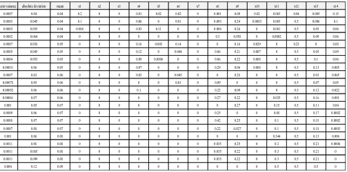
Table 3: Results from solving the model (mean – semi variance - absolute deviation) with probable constraints along with the percentage of investment per stock

x14 x13 x12 x11 x10 x9 x8 x7 x6 x5 x4 x3 x2 x1 mean absolute deviation semi variance 0.15 0.005 0.04 0.003 0.02 0.09 0.001 0 0.02 0.02 0.01 0 0 0.2 0.04 0.04 0.0007 0.1 0.006 0.5 0.003 0.0003 0.24 0.003 0 0.01 0 0.06 0 0 0.1 0.04 0.045 0.0003 0.06 0.05 0.5 0.001 0 0.26 0.006 0 0 0.11 0.03 0 0 0.008 0.04 0.055 0.0003 0.06 0.09 0.5 0.0002 0 0.058 0.3 0 0 0 0 0 0 0 0.04 0.064 0.0002 0.08 0 0.23 0 0.029 0.16 0 0 0.14 0.003 0.16 0 0 0 0.05 0.038 0.0007 0.09 0.05 0.5 0 0.007 0.21 0.06 0 0.044 0 0.12 0 0 0 0.05 0.045 0.0005 0.06 0.1 0.5 0 0.008 0.22 0.06 0 0 0.0006 0.09 0 0 0 0.05 0.053 0.0004 0.005 0.13 0.5 0 0.008 0.06 0.29 0 0 0 0.07 0 0 0 0.05 0.06 0.00031 0.065 0.03 0.5 0 0 0.28 0 0 0.045 0 0.03 0 0 0 0.06 0.03 0.0007 0.05 0.07 0.5 0 0 0 0.09 0 0.01 0 0 0 0 0 0.06 0.05 0.00078 0.022 0.12 0.5 0 0 0.09 0.22 0 0 0 0.1 0 0 0 0.06 0.06 0.00052 0.001 0.16 0.5 0.035 0 0.22 0.27 0 0 0 0 0 0 0 0.06 0.07 0.00061 0.04 0.11 0.5 0.15 0 0.27 0 0 0 0 0 0 0 0 0.07 0.05 0.001 0.0002 0.17 0.5 0.08 0 0 0.25 0 0 0 0 0 0 0 0.07 0.06 0.0009 0.0002 0.18 0.5 0.1 0 0.25 0.42 0 0 0 0 0 0 0 0.07 0.07 0.0008 0.0003 0.18 0.5 0.1 0 0.027 0.22 0 0 0 0 0 0 0 0.07 0.08 0.0007 0.006 0.13 0.5 0.344 0 0 0 0 0 0 0 0 0 0 0.08 0.06 0.001 0.0006 0.21 0.5 0.3 0 0.25 0.035 0 0 0 0 0 0 0 0.08 0.08 0.0011 0 0.21 0.5 0.3 0 0.22 0.035 0 0 0 0 0 0 0 0.08 0.085 0.0011 0 0.21 0.5 0.3 0 0.22 0.035 0 0 0 0 0 0 0 0.08 0.099 0.0011 0 0.5 0.5 0.5 0 0 0 0 0 0 0 0 0 0 0.09 0.12 0.004 CONCLUSIONS

We mentioned an important constraint called probable constraint. In real probable constraint is the investor’s amount of sureness that he achieved the specified expected return of

portfolio. Regarding the available stocks nearly the optimum portfolios consist of all the

stocks.

Considering the above points, the best reason for offering integrated models

is simultaneous use of two measures of risk and making models more realistic by adding the

trading costs constraint in order to obtain a better result for investors. In terms

of investors, the proposed model is preferred over common models, because of

multi-dimensional and better answers than the other methods. On the other hand, the proposed

model is more quickly than other, because the problem can be solved using linear

programming and it causes the reduction of solvable problems which can decrease the cost

and time of decision making for investors. Then, by studying the tables obtained from solving

multi objective model with probable constrain and trading costs, it is observed that focus

on one or more specific stock has been removed and scattered on the whole portfolio. Also by

comparing the diagrams obtained from solving this multi objective model and other simple

(15)

GE-International Journal of Management Research (GE-IJMR) ISSN: (2321-1709)

93 | P a g e

trading cost is lower. It means that by changing the value of

a risk measure, other measure will have lower changes. Therefore, the risk fluctuation of

portfolio for the investor is less than the past. Finally, it can be concluded that multi

objective models, represent an appropriate and comprehensive information package

to investors and managers in order to better manage risk.

According to the analysis of models and process of solve the recommendations for future are

as below:

1. In solving process with the probable model we assume that the past return have

normal distribution; maybe this point will not be true. So we propose to solve the

model with this assumption that the past returns have other distribution except

normal.

2. Application mathematical programming depending on the decision of the decision

maker. So insert new constraints maybe result better answers.

REFERENCES

1. Charnes, A., Cooper, W. W. (1959). Chance-constrained programming. Management

Science, 6(1):73-79.

2. Feiring, B. R., Lee, S. W. (1996). A chance-constrained approach to stock selection in

hong kong. International Journal of Systems Science, 27(1):33-41.

3. Kandasamy, Hari, (2008), Portfolio Selection under Unequal Prioritized Downside Risk,

Advisor: Kostreva, Michael M., the Degree Doctor of Philosophy Mathematical

Sciences, Department of Mathematical Science, Clemson University.

4. Konno, H.,Yamazaki, H. (1991). Mean-absolute deviation portfolio optimization model

and its applications to tokyo stock market. Management Science, 37(5):519-531.

5. Manganelli, S., Engle, R.F., (2011). Value at risk models in finance. European Central

Bank, Working paper.

6. Markowitz, H. (1952). Portfolio selection. Journal of Finance, 7(1):77-91.

7. Markowitz, H. (1959). Portfolio Allocation: E_cient Diversi_cation of Investments, John

Wiley & Sons, Inc., New York. A Cowles Foundation Monograph.

8. Markowitz, H. (1991). Foundations of portfolio theory. Journal of Finance,

(16)

GE-International Journal of Management Research (GE-IJMR) ISSN: (2321-1709)

94 | P a g e

9. Papahristodoulou, C, Dotzauer, E. (2004). Optimal portfolios using linear programming

problems. Journal of the Operations Research Society, 55(11):1169-1177.

10. Rockafellar, R. T., Ursayev, S. (2010). Optimization of Conditional Value-at-Risk. The

Journal of Risk, 2(3):21- 41.

11. Roman, D., Dowman, K. D., Mitra, G. (2007). Mean risk models using two risk

measures: A multi-objective approach. Quantitative Finance, 7(4):443 -458.

12. Speranza, M. Grazia. (1995). A Heuristics Algorithm for A Portfolio Optimization

Model Applied To the Milan Stock Market, Computer and Ops Res, 5,.433-441.

13. Tang, W., Han, Q., Li, G. (2001). The portfolio selection problems with

chance-constrained. In Systems, Man, and Cybernetics IEEE International Conference on,