MODELLING AND OPTIMISING THE TRANSHIPMENT PROBLEM OF NAGAPATTINAM MUNICIPALITY SOLID WASTE MANAGEMENT

(1)

MODELLING AND OPTIMISING THE TRANSHIPMENT PROBLEM OF

NAGAPATTINAM MUNICIPALITY SOLID WASTE MANAGEMENT

Dr. R. Sophia Porchelvi,

(1)

Associate professor,Dept of Mathematics, A.D.M College for women, Nagapattinam 611001,TamilNadu,India.

P. Jamuna Devi,

(2)

Assistant Professor,Dept of Mathematics, E.G.S.Pillay Engineering College , Nagapattinam 611001,TamilNadu,India.

ABSTRACT

There is a need for mathematical tools in order to manage the municipal solid waste and thereby

providing a healthy environment to the society. The transportation problem is a special class of

the linear programming problem. It deals with the situation in which a commodity is transported

from Sources to Destinations. The transshipment problem is an expansion of the transportation

problem where intermediate nodes which are also referred to as transshipment nodes are added

to account for locations such as warehouses. The flow of waste from the source spot through

processing spot to the destination spot has been formulated alternatively as a transshipment

model. The main objective of this paper is to model solid waste management as a transshipment

problem and also minimize the cost in transporting them. Transshipment problem has been

formulated to a Transportation problem algorithm and TORA Software has been used to

analyze the data. If Nagapattinam municipality adapts this method, the cost of transporting

waste will be minimized also the waste will be processed in the processing plants and its

by-product will be used in the market and the total quantity sent to the dumping yard will be

reduced which will help in increasing the life span of dumping yard.

Keywords: MSW-TSP model- Optimal Solution- Case Study

(2)

About 55 million tonnes of Municipal Solid Waste (MSW) and 38 billion liters of sewage

are generated in the urban areas of India. It is estimated that the amount of waste generated in

India will increase at a per capita rate of approximately 1-1.33% annually. The Ministry of New

and Renewable Energy has predicted that there exists a power generation potential of about 1500

MW from the MSW generated in India and the Indian Government is actively promoting the

waste to energy technologies, by providing various incentives and subsidies for waste to energy

projects. But according to the Indian Renewable Energy Development Agency (IREDA), only

2% of the potential has been tapped in India so far. Nagapattinam district is an eastern coastal

region of Tamilnadu, India. Major population depends on fishing and its by-products. In every

value addition stage of improving the quality of sea foods, leads to lots of wastage. In the boat

house and fish markets tones of fish waste due to improper size or poor quality are collected.

44% of the waste is collected from residential areas. 19% from hospitals,17% from fish market,

11% from commercial areas and 9% waste from institutional areas. At present, waste is disposed

off through dumping in a disposal yard outside the town. The disposal yard is situated at a

distance of 5 km from the town and it is spread over 19 acres. The disposal yard is sufficient for

another 15 years. The disposal is done only through dumping. Nagapatinam municipality is in

the process of implementing measures to develop the dumping yard and implement composting.

Waste management is necessary for every country because it directly affects the health of

the people and environment. In Nagapattinam town, dengue breaks out in rainy season due to the

mosquitoes for which the garbage is the dwelling place. It spreads many diseases like malaria,

cholera, typhoid, chikunkunia etc., The municipal solid waste mixes up with the river water

which affects the quality of water. It also affects the living organisms like fish. The nutrients

from the waste make the river and lakes a better place to grow for water hyacinth and other

unwanted weeds, which leads to loss of water sources. From the rotten garbage, toxic gases

emerge out which is deadly to human beings, animals and plants. As population grows year by

year, there will be a scarcity in land which is used for disposal. Therefore there is an urgent need

for solving all those problems. Solid waste management by mathematical models will be

definitely useful for decision makers for reducing waste, for minimizing travelling cost and also

(3)

MSW-TSP MATHEMATICAL MODELLING:

The objective of transportation problem is to transport various quantities of a single homogenous

commodity from the origin to different or one single destination with the aim to reduce the

transportation cost. To achieve this one should know the capacity and location of source and

destination. Along with that the cost of transporting one unit of goods from various origin to

various destination must also be known. In addition to this there exist points through which units

of goods can be transshipped from source to destination. Models with this additional feature is

called transshipment model. The transshipment technique is used to find the shortest route from

one point to another point representing network diagram. The flow of waste from the source spot

through processing spot to the destination spot has been formulated alternatively as a

transshipment model. The transshipment model to manage municipal solid waste is termed as

MSW-TSP model. The MSW-TSP model is a network in a linear form which owes to minimize

the transportation cost. In this paper we have discussed a simple method for solving MSW by

transshipment model for arriving optimal solution.

Source spot: Source spot is nothing but it can send all the waste materials to another spot say

processing plant, dumping yard but cannot receive waste materials from other place.

Destination spot: Destination spot is a spot which can receive waste or recoverable waste from

other points but it cannot send materials to another spot. In our study dumping yard and market

are the destination points.

TSP spot: This is nothing but it can both collect waste materials from some points and also send

the waste or recovered material to other points. In our study processing plants, separators are

(4)

Let the source be represented as A and destination as Z , then Xaz represents the amount of waste

transported from ath position Aa to the zth position Zz and Caz represent the cost for transporting unit mass of waste material where Xaa and Xzz both are zero since no material would be

transported from a to a or z to z. Assume m terminals A1,A2,… Am the total out shipment exceeds the total in shipment by amounts OS1,OS2,… OSm respectively and at the remaining n terminals Am+1, Am+2,…. Am+n the total in shipment exceeds the total out shipment by amounts

ISm+1, IS m+2,… IS m+n respectively. The total in shipment at terminals A1, A2,… Am be t1,t2,t3..tm and total outshipment at terminals Am+1,Am+2…. Am+n be tm+1,tm+2,…tm+n respectively.

𝑀𝑖𝑛𝑖𝑚𝑖𝑧𝑒 𝐶𝑜𝑠𝑡 = 𝐶𝑖𝑗 𝑋𝑖𝑗

𝑛

𝑗 𝑚

𝑖

Subject to the supply constraint 𝑋𝑖𝑗𝑛𝑗 ≤ 𝑆𝑖 , 𝑖 = 1,2,3 … 𝑛

And demand constraint 𝑋𝑖𝑗𝑚_𝑖 ≥ 𝐷𝑗, 𝑗 = 1,2,3 … 𝑚

Transshipment constraint 𝑋𝑖𝑗𝑛_𝑖 − 𝑋𝑖𝑗𝑚_𝑗 ≥ 0

In the transshipment node the waste will be processed and the useful material will be sent to the

market.ie Output from transshipment node necessarily need not be equal to the total quantity

from the source.

(5)

This section deals with data collection, data analysis and discussion, the discussion of transshipment of waste from sources to the landfill. The data was collected from Nagapattinam

Municipality Office and Official Website of Nagapattinam town. The cost of transporting waste

involves fuel consumption of vehicles and labour cost. At present there is two dumping yard, one

in the outer skirt of the Nagapattinam town and another near Nagur bridge. There are no

processing plants at Thethi, Sellur and Akkaraipet. All the waste from sources is directly taken to

the landfill except very negligible quantity to the compost near the landfill. In this paper

decisions are basically based on intuition and experience. Consider the following transshipment

model involving 4 sources and 3 destinations with 3 transshipment nodes. The supply value of

the sources be s1, s2, s3 and s4.

Zone 1 – Nagur(NG)

Zone 2- Vellipalayam(VL)

Zone 3- kottavasappadi(KT)

Zone 4- Keechankuppam and Akkaraipet (KE)

And three destination spot – ie the dumping yard , where all the wastages are taken.

DumpingYard 1- Nagapattinam outer (NO)

Dumping yard 2- Andanappetai outer (AO)

Dumping Yard 3- Nagur Bridge outer(NB)

Before taking all the waste directly to dumping yard, they are carried to the processing plants

(incinerator, compost, biofuel plant) which acts as transshipment node.

TSP node 1- Sellur (SL)

TSP node 2-Akkaraipet(AK)

(6)

The transportation cost per unit between different sources and destination are given in a

generalized matrix form.

S1 S2 S3 S4 P1 P2 P3 D1 D2 D3

S1 0 CNG-VL CNG-KT CNG-KE CNG-NO CNG-AO CNG-NB CNG-SL CNG-AK CNG-TT

S2 CVL-NG 0 CVL-KT CVL-KE CVL-NO CVL-AO CVL-NB CVL-SL CVL-AK CVL-TT

S3 NG VL 0 KE NO AO NB SL AK

CKT-TT

S4 CKE-NG CKE-VL CKE-KT 0 CKE-NO CKE-AO CKE-NB CKE-SL CKE-AK CKT-TT

P1 CNO-NG CNO-VL CNO-KT CNO-KE 0 CNO-AO CNO-NB CNO-SL CNO-AK CNO-TT

P2 CAO-NG CAO-VL CAO-KT CAO-KE CAO-NO 0 CAO-NB CAO-SL CAO-AK CAO-TT

P3 CNB-NG CNB-VL CNB-KT CNB-KE CNB-NO CNB-AO 0 CNB-SL CNB-AK C

NB-TT

D1 CSL-NG CSL-VL CSL-KT CSL-KE CSL-NO CSL-AO CL-NB 0 CSL-AK C

SL-TT

D2 CAK-NG CAK-VL CAK-KT CAK-KE CAK-NO CAK-AO CAK-NB CAK-SL 0 C

AK-TT

D3 CTT-NG CTT-VL CTT-KT CTT-KE CTT-NO CTT-AO CTT-NB CTT-SL CTT-AK 0

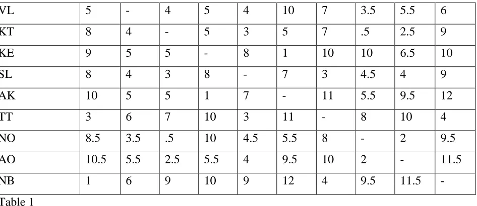
The following table shows the distance between the locations in Kilometers

NG VL KT KE SL AK TT NO AO NB

(7)

VL 5 - 4 5 4 10 7 3.5 5.5 6

KT 8 4 - 5 3 5 7 .5 2.5 9

KE 9 5 5 - 8 1 10 10 6.5 10

SL 8 4 3 8 - 7 3 4.5 4 9

AK 10 5 5 1 7 - 11 5.5 9.5 12

TT 3 6 7 10 3 11 - 8 10 4

NO 8.5 3.5 .5 10 4.5 5.5 8 - 2 9.5

AO 10.5 5.5 2.5 5.5 4 9.5 10 2 - 11.5

[image:7.612.74.547.84.289.2]

NB 1 6 9 10 9 12 4 9.5 11.5 -

Table 1 Source:Google Map

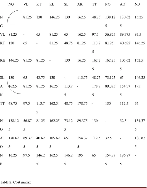
The following table shows the fuel consumption cost (in Rs) on every movement made. Assume

the vehicles involved in collecting and disposing waste are of same capacity and same type with

same efficiency. During this study (2014)1 liter of Diesel costs Rs 62.50. The labour cost is also

added for calculating the cost matrix. The Shipping cost is obtained by multiplying the cost per

(8)

NG VL KT KE SL AK TT NO AO NB

N

G

- 81.25 130 146.25 130 162.5 48.75 138.12

5

170.62

5

16.25

VL 81.25 - 65 81.25 65 162.5 97.5 56.875 89.375 97.5

KT 130 65 - 81.25 48.75 81.25 113.7

5

8.125 40.625 146.25

KE 146.25 81.25 81.25 - 130 16.25 162.2

5

162.25 105.62

5

162.5

SL 130 65 48.75 130 - 113.75 48.75 73.125 65 146.25

A

K

162.5 81.25 81.25 16.25 113.7

5

- 178.7

5

89.375 154.37

5

195

TT 48.75 97.5 113.7

5

162.5 48.75 178.75 - 130 112.5 65

N O 138.12 5 56.87 5

8.125 162.25 73.12

5

89.375 130 - 32.5 154.37

5 A O 170.62 5 89.37 5 40.62 5 105.62 5

65 154.37

5

112.5 32.5 - 186.87

5

N

B

16.25 97.5 146.2

5

162.5 146.2

5

195 65 154.37

5

186.87

5

[image:8.612.72.543.106.707.2]

-

(9)

Sources: Secondary data from Nagapattinam Municipality office and Website

The following table shows the cost matrix in Rs. Supply availability is shown at the far right

column and demand is shown at the bottom row. Overall the solid waste generated ads up to 55

tones with a collection efficiency of 75.22 per cent with a manpower of 111 for Solid waste

management. On the basis of the figures furnished by Nagapattinam municipality, it was

observed that 85 per cent of the solid wastes are compostable on wet basis and 15 per cent of

rags, plastics, etc. are not compostable in the district.

Total supply= 55 movements

Total Demand= 55 movements

One movement = 1000 Kg= 1 ton of waste.

D1 D2 D3 D4 D5 D5

S1 130 162.5 48.75 138.125 170.625 16.25

S2 65 162.5 97.5 56.875 89.375 97.5

S3 48.75 81.25 113.75 8.125 40.625 146.25

S4 130 16.25 162.25 162.25 105.625 162.5

S5 - 113.75 48.75 73.125 65 146.25

S6 113.75 - 178.75 89.375 154.375 195

S7 48.75 178.75 - 130 112.5 65

Table:3

Pure Sources: S1, S2,S3,S4

Transhipment Nodes: S5,S6,S7

Pure destination: D4 , D5, D6

(10)

Optimal solution to this problem can be found using the following steps.

Make the problem a balanced one by adding dummy such that supply matches the demand.

Shipment from a point to itself will be zero. If any dummy is added, shipment to a dummy is also

zero.

Each transshipment point will have a supply equal to the points original supply and a demand

equal to its original demand. Total amount transshipped will not exceed the total supply S.

To form the transshipment table , the route from source to destination through processing plants

which takes minimum cost is chosen.

Cost cell S1D1= Min(S1P1D1,S1P2D1,S1P3D1)=Min(203.125,251,875,178.75)= 178.75

Cost cell S1D2= Min(S1P1D2,S1P2D2,S1P3D2)=Min(195,316.875,211.25)= 195

Cost cell S1D3= Min(S1P1D3,S1P2D3,S1P3D3)=Min(276.25,357.5,113.75)= 113.75

(11)

Cost cell S3D1= Min(S3P1D1,S332D1,S1P3D1)=Min(121.875,170.625,243.75)= 121.875

Cost cell S3D3= Min(S3P1D3,S3P2D3,S3P3D3)=Min(195,276.25,178.75)= 178.75

Cost cell S4D2= Min(S4P1D2,S4P2D2,S4P3D2)=Min(195,170.625,324.75)= 170.625

TABLE:4

D1

D2

D3

SUPPLY

S1

178.75

195

113.75

7 S2

138.125

130

162.5

12 S3

121.875

113.75

178.75

16 S4

103.625

170.625

211.25

20 DEMAND

22

17

16

55

This problem can be modeled as

178.75 X11 + 195 X12 + 113.75 X13

138.125X21+ 130 X22 + 162.5 X23

121.875 X31 +113.75 X32 +178.75 X33

103.625 X41 +170.625 X42 +211.25 X43

(12)

X21+ X22 +X23 = 12

X31+ X32 +X33 = 16

X41+ X42 +X43 = 20

X11+X21+X31+X41= 22

X12+X22+X32+X42= 17

X13+X23+X33+X43= 16

COMPUTATIONAL PROCEDURE:

For calculation TORA software WINDOWS 8 version and 64 bit capacity and HP computer with

500 GB as hard disk size 4 GM DDRZ Ram has been used.

The initial basic feasible solution is

Capacity K =( XB11,X12,X13,XB21,X22,X23,XB31,XB32,X33,X41,XB42,XB43)

= (178.75,0,0,138.125,0,0,121.875,113.75,0,0,170.625,211.25)

Total cost= Rs 8815.625

Next we use the optimality condition to improve the solution using MODI method

Cij=Ui +Vj

Consider U1=0 we get

V1=89.375, U2=48.75, V2=81.25, U3=32.5, V3=113.75, U4=14.25

At the end of iteration , the basic feasible solution is

Capacity K= (0,0,113.75, 0,162.5,121.875, 113.75,0,103.625,0,0)

(13)

REFERENCE

1. Arul P asian Tsunami Ecological implication and Rehabilationprocesses along

Nagapattinam coast 2012

2. Asmuth R., Curtis E. B. and Peterson E. L. (1979).Computing Economic Equilibria on

Affine Networks with Lemke's Algorithm. Journal of the institute of operations research

and management sciences

3. Bruce H. and Tardos E. (1997). The Quickest Transshipment Problem Journal of the

institute of operations research and management science

4. Dahan E. (2009). The Transshipment Problem with Partial Lost Sales. M.Sc Thesis

Department of Industrial Engineering and Management Isreal institute of technology.

5. De Rosa B., Improta G., Gianpaolo G. and Musmanno R. (2001).The Arc Routing and

Scheduling Problem with Transshipment. Journal of the institute of operations research

and management sciences

6. George Marfo Ofori 2012 Modelling the distribution of bank notes by banh of Ghana as a

transshipment problem, Kwame Nkrumah University of Science and Technology

7. Glover F., Karney D., Klingman D. and Russell R. (2005). Solving Singly Constrained

Transshipment Problems. Journal of the institute of operations research and management

science

8. Gong Y. and Yucesan E. (2006).The Multi-Location Transshipment problem with

Positive Replenishment Lead Times. ERIM Report Series Reference No.

ERS-2006-048-LIS

9. Hanany E., Tzur M., and Levran A. (2010).The transshipment fund mechanism:

Coordinating the decentralized multilocation transshipment problem

10.Hezarkhani B. and Wiesław K. (2010). Transshipment prices and pair-wise stability in

coordinating the decentralized transshipment problem. Proceedings of the Behavioral and

Quantitative Game Theory: Conference on Future Directions

11.Horowitz A. (2009). The Transshipment Problem. Masters degree Thesis,Department of

Civil Engineering and Mechanics University of Wisconsin – Milwaukee

(14)

13.Orden A. (1956). The Transhipment Problem. Journal of the institute of operations

research and management science vol. 2 no. 3 276-285

14.Ozdemir D., Yucesan E, and Herer Y. T. (2003). A Monte Carlo simulation approach to

the capacitated multilocation transshipment problem. Simulation Conference report.

Proceedings of the 2003 Winter.

15.Perincherry V. and Kikuchi S. (1990). A fuzzy approach to the transshipment problem.

Uncertainty Modeling and Analysis, First International Symposium

16.Topkis, D.M(1984). Complements and Substitutes among Locations in the Two-Stage

Transhipment Problem. European Journal of Operational Research, ISSN: 0377-2217.

17.Xiao H. and Greys S.(2008).Transshipment of Inventories: Dual Allocations vs.

Transshipment Prices. http://msom.journal.informs.org/content

18.Yale T. H. and Tzur M., (2001). The dynamic transshipment problem. Journal of Naval

Research Logistics (NRL). Fleischer L. (1997). A Faster Algorithm for the Quickest

Transshipment Problem. Proceedings of the Ninth nnual ACM/SIAM Symposium on