Original Citation:
Coupling different methods for overcoming the class imbalance problem
Publisher:
Published version:
DOI:
Terms of use:
Open Access
(Article begins on next page)
This article is made available under terms and conditions applicable to Open Access Guidelines, as described at http://www.unipd.it/download/file/fid/55401 (Italian only)
Availability:
This version is available at: 11577/3156786 since:
10.1016/j.neucom.2015.01.068
Università degli Studi di Padova
1
Coupling different methods for overcoming the class imbalance
problem
Loris Nanni, Carlo Fantozzi, Nicola Lazzarini
DEI, University of Padua, Via Gradenigo, 6 - 35131- Padova – Italy
Abstract. Many classification problems must deal with imbalanced datasets where one class – the majority class – outnumbers the other classes. Standard classification methods do not provide accurate predictions in this setting since classification is generally biased towards the majority class. The minority classes are oftentimes the ones of interest (e.g., when they are associated with pathological conditions in patients), so methods for handling imbalanced datasets are critical.
Using several different datasets, this paper evaluates the performance of state-of-the-art classification methods for handling the imbalance problem in both binary and multi-class datasets. Different strategies are considered, including the one-class and dimension reduction approaches, as well as their fusions. Moreover, some ensembles of classifiers are tested, in addition to stand-alone classifiers, to assess the effectiveness of ensembles in the presence of imbalance. Finally, a novel ensemble of ensembles is designed specifically to tackle the problem of class imbalance: the proposed ensemble does not need to be tuned separately for each dataset and outperforms all the other tested approaches.
To validate our classifiers we resort to the KEEL-dataset repository, whose data partitions (training/test) are publicly available and have already been used in the open literature: as a consequence, it is possible to report a fair comparison among different approaches in the literature. Our best approach (MATLAB code and datasets not easily accessible elsewhere) will be available at https://www.dei.unipd.it/node/2357.
2
Keywords: imbalanced dataset; ensemble of classifiers; support vector machine; downsampling/oversampling.
1.
Introduction
Highly imbalanced datasets are not uncommon in many pattern recognition tasks [3][4]. For example, in medical datasets instances of diseased patients are typically rarer than instances of sane individuals. Yet, it is the rare cases that attract the most interest, as detecting them enables patients to be diagnosed and treated. Similar needs also appear in other real-world applications such as anomaly detection, fault diagnosis, email foldering, face recognition, fraud detection.
In binary classification, the under-represented class is called the minority class or positive class. The other class, which contains the vast majority of the members, is referred to as the
majority class or negative class. When the class distribution is asymmetric, regular classifiers – such as support vector machines (SVMs) – tend to ignore data in the minority class and treat them as noise, resulting in a class boundary that unduly benefits the majority class. In turn, this produces a drop in precision when classifying the minority class [5].
A common approach in m-class learning, with m greater than 2, is the one-against-all method:
the original problem is decomposed into m binary classification instances, where each class is in
turn labeled as positive and the remaining m-1 as negative. Unfortunately, this method aggravates
the issue of imbalance in each of the m instances. As a consequence, ad-hoc systems for handling
multi-class imbalanced problems must be developed [4]. In the rich literature on imbalanced
classification, the most common methods employed [6-13] are undersampling of the majority
class, oversampling of the minority classes, ensemble methods, cost-sensitive learning,
asymmetric classification, dimension reduction.
The simplest approach to undersampling is to randomly select a fraction of records from the
majority class. Unfortunately, this may lead to a loss of useful information. An interesting
3
BalanceCascade. In EasyEnsemble,the majority class is sampled into several independent subsets that are used to train separate classifiers, whose outputs are finally combined to produce the
classification decision. In BalanceCascade, trained models are used to guide the sampling process
for succeeding classifiers. The system is more focused on training patterns that are hard to classify. The main drawback of these preprocessing algorithms is that, again, potentially useful data from the majority class may not be considered.
As far as oversampling is concerned, the basic approach is to randomly duplicate the records
in the minority classes to increase the cardinality of the classes themselves. A very popular approach is SMOTE (Synthetic Minority Oversampling TEchnique), which increases diversity by generating pseudo minority class data [14]. Several variants of SMOTE have been proposed: among them, we cite Borderline-SMOTE [64], MSMOTE [15], and the recent MWMOTE [60]. In [59] the imbalance problem is tackled by generating artificial instances, using an evolutionary framework, in order to modify the class ratio in the original dataset. A further interesting approach is RAMOBoost, introduced in [37] for binary classification. This technique oversamples the minority class using an adaptive weight adjustment procedure that shifts the decision boundary towards the difficult-to-learn examples from both the minority and majority classes.
Boosting (see also [20][21][41][58]) and other ensemble methods, such as Bagging
[17][18][19][22], have proved to be particularly robust at handling imbalanced data. A recent review on ensemble methods applied to handle the class imbalance problem is [55]. AdaBoost [65], for instance, is designed to reduce the bias towards the majority class by focusing on misclassified
training patterns [20], while Bagging introduces the concept of bootstrap aggregating [19] that
consists in training several classifiers with bootstrapped copies of the original training set. Ensemble classifiers by themselves do not ameliorate the issue of imbalance if they are directly applied on data: this is due to their accuracy-oriented design. However, their combination with other techniques leads to positive results. Some examples are: SMOTEBoost [21], SMOTEBagging [22], IIVotes [23][51], RUSBoost [41]. In these approaches, a data-preprocessing algorithm is applied
4 before bagging/boosting, hence a 3-step process can be identified: resampling, ensemble building, and voting for the final classification. IRUS [24] is a method that couples random undersampling and Bagging. The main idea behind it is to create bags where the majority class is so severely under-sampled that the imbalance situation is reversed with respect to the original one. Each bag contains all the positive patterns but only a few negatives: in this way, the focus of classification is on the minority class, which can be successfully separated from the majority class.
Another group of classifiers is based on cost-sensitive learning. In this approach, a different
cost is assigned to false negative and false positive patterns. SVM-WEIGHT implements
cost-sensitive learning for SVM modeling [38]. It is implemented in LIBSVM1, so it is a very interesting
baseline. The cost-sensitive principle is also applied in [44] to the ELM classifier.
A number of recent studies have focused on the development of asymmetric classifiers [24].
The main difference with cost-sensitive classification is that asymmetric classifiers are not exclusively focused on assigning a different weight to false negative and false positive patterns. Chew et al. [26] propose an unbalanced SVM (called UnSVMs in their paper) to adjust the error penalties of each class. Granular SVM is proposed in [27]: it resorts to a repetitive undersampling method where information loss is minimized and the undersampling process maximizes the positive effect of data cleaning.
Some researchers have focused on improving dimension reduction methods, such as
principal component analysis (PCA) and linear discriminant analysis (LDA), as a way of handling imbalanced data sets [28][29][30]. The key idea behind many of these methods is the eigen decomposition problem, which is tightly bound with data structure and class distribution, where the latter is asymmetric when data are skewed. To offset the effects of imbalanced data when applying PCA, an asymmetric principal component and discriminant analysis (APCDA) method was successfully employed in [28]. It is also worth to mention the method proposed in [34], where the
5 authors implement an asymmetric classifier based on partial least squares (PLS) [33] to generate a new classification hyperplane and tackle the imbalance.
In recent years, some methods based on plain SVM have been proposed as well. For instance, in [38] a method called VQSVM is introduced. It is well known that SVM selects a subset of training patterns and uses them as the set of support vectors within the decision function. In VQSVM, vector quantization replaces the original set of support vectors with a subset, so that the number of instances belonging to the majority class is reduced.
In this paper, our aim is twofold.
1. We study the fusion among different approaches for handling the imbalance in the
datasets following the “ensemble of ensembles” strategy.
2. We propose a new ensemble method, called HardEnsemble, to overcome the problems
of existing approaches (e.g. parameters tuning, removal of potentially informative patterns, generation of new outliers, etc.). HardEnsemble provides good performances with both 2-class and multi-class datasets. Note that previous works were commonly focused only one of the two types of datasets, while we cover both.
To validate our results we test many state-of-the-art approaches using more than 40 datasets. In order to properly evaluate the results we employ a statistical test, the Wilcoxon signed-rank test, as commonplace in the open literature when it is necessary compare algorithms over multiple datasets [2].
2.
Tested Approaches
The aim of this paper is to find a set of approaches that works well with several datasets: to be precise, we want to determine whether some fusion of different classifiers for handling the imbalance problem consistently outperforms each of the classifiers when taken in isolation. We have tested methods based on different approaches, e.g. cost-sensitive learning, oversampling of the
6 minority classes, and undersampling of the majority class. In all cases, an SVM is used as the base classifier unless differently specified.
In this section we give a technical summary of the approaches that have been previously presented in the open literature and included in our investigation; a separate subsection is devoted to each approach.
2.1 Asymmetric PLS Classifier (APLSC)
APLSC is an asymmetric partial least squares (PLS) classifier [34] which complexly
researches into the skewed distribution between classes and is prone to give high accuracy to the minority class in the cost of poor performances on the majority class. It can be summarized into two steps:
• feature extraction performed using PLS method [33] on normalized feature vectors;
• classification of compressed vectors by translated hyperplane, that is influenced by the
variance of low dimensional data.
2.2 One-class SVM (OCSVM)
One-class SVM is an adaptation, proposed by Scholkpof [40], of SVM to one-class classification problem. SVM is usually constructed as a two-class algorithm, OCSVM can be viewed as a regular two-class SVM where all training data belong to the first class and the origin point of the space is the only member of the second class. The idea of OCSVM is to map the input into high dimensional feature space using a kernel function and then define a hyperplane that best
separates the class with maximum margin. Given a training set , let us define as the
function which maps the data point from the input space to the feature space F. To separate
7 constrained to:
where w is a vector perpendicular to the hyperplane and is the distance from the origin. As usual in SVM, the slack variable allows for error in classification. The parameter ν ∈ (0, 1]
controls the tradeoff between the number of examples of the training set mapped as positive and the
complexity of the model defined by small values of .
2.3 K-Nearest neighbor data generation (GK)
GK is a method that generates artificial examples using k-nearest neighbors of samples in the
dataset [52]. This allows reducing the ratio between classes in imbalanced datasets. The first m
points are randomly chosen from the dataset, then to each of these points and for each space direction (feature) a Gaussian distributed offset with zero mean is added. The standard deviation is
obtained by multiplying the input parameter s with the mean signed difference between the
considered point in the dataset and its i-th nearest neighbor. In this way the generated points follow
the local density properties of the original points from whom they are created.
2.4 Modified SMOTE (MSMOTE)
MSMOTE is a modified version of SMOTE [14], an algorithm that creates minority synthetic samples by randomly interpolating pairs of closest neighbors which belong to the minority class.
MSMOTE divides minority class examples into three groups – safe, border and noise – based on
the label of their k-nearest neighbors. If all neighbors belong to the minority class, then the sample
is considered safe; if all neighbors belong to other classes, then the sample is noise, otherwise it is
treated as border. If the sample is safe then MSMOTE randomly chooses one of the k-nearest
neighbors, if it is border it selects the nearest neighbor, while for noise samples it does nothing. The
main improvement, with respect to the original SMOTE, is to reject latent noisy spots for the creation of new synthetic samples.
8
2.5 RUSBoost
RUSBoost [41] is an algorithm that combines data sampling and boosting. It is a variant of SMOTEBoost [21]. SMOTEBoost creates new synthetic examples for the minority class by using SMOTE, while RUSBoost realizes a Random UnderSampling (RUS) by removing examples from the majority class. RUSBoost is really similar to AdaBoost: first the weights of each example are initialized to 1/m, where m is the number of total examples in training set, then for T times (iterations) a training set is created by applying Random Undersampling on the original majority set. Compared to SMOTEBoost, this algorithm is less computationally complex and time consuming. Results in [41] show that on average RUSBoost significantly outperforms SMOTEBoost.
2.6 EasyEnsemble
EasyEnsemble is a method proposed in [13] that aims at overcoming the main deficiency of oversampling: many examples of the majority class are discarded and not considered. The idea
behind EasyEnsemble is to create an ensemble of T classifiers trained on different training sets. Let
us define P and N as the subsets of positive and negative examples, respectively: each training set is
created by using all positive examples and randomly selecting (with replacement) negative
instances from N. The number of negative selected examples is usually |P|, so that each training set
has a size of 2|P|. In this way, EasyEnsemble creates T balanced sub-problems, each of them used to
train an Adaboost classifier .
2.7 BalanceCascade
BalanceCascade is an ensemble learning method that relies on undersampling as the strategy to deal with an imbalanced dataset while avoiding the already stated flaw of undersampling: it can discard useful data. BalanceCascade addresses this issue by exploring majority class examples ignored by the undersampling process. BalanceCascade employs Bagging [53] and uses Adaboost as base learner: as a consequence, the final model can be considered an “ensemble of ensembles”.
9
The main idea behind BalanceCascade is as follows: if an example (subset of training
examples that belongs to the majority class) is correctly classified by , during the i-th iteration, it
is reasonable to speculate that x is “redundant” in N, because there already exists a classifier to classify it. Hence, it is possible to remove it from N so that further classifiers do dot take it into
account. In [13] it is stated that BalanceCascade offers higher AUC, F-measure and G-mean than
almost all methods commonly used to manage data imbalance.
2.8 IRUS
The main idea behind IRUS (Inverse Random UnderSampling) [24] is to reverse the ratio between majority and minority class cardinality by severely undersampling the majority class multiple times. IRUS is an ensemble learning method that relies on bagging. Using only few
majority class examples leads to a high true positive rate (tpr) but also to a high false positive rate
(fpr) since the number of negative examples is much lower than the number of positives. By
combining classifiers obtained from different bags (trained on different datasets), the false positive rate is controlled.
2.9 OverBagging
OverBagging [3] is a method for the management of class imbalance that merges bagging and data preprocessing. The whole procedure can be described with 3 steps: resampling, construct ensemble, fuse classification outputs. There are two ways to implement this solution. The first procedure allows to increase the cardinality of the minority class by replication of original examples, while the examples in the majority class can be all considered in each bag or can be resampled to increase the diversity. A second way to oversample the minority class can be obtained by resorting to the SMOTE algorithm: the resulting method, called SMOTEBagging [3], differs from OverBagging in how bags are populated: first each class is resampled with replacement at
percentage 100%, then SMOTE is applied to the minority class with a resample rate of b%. The
10 multiple of 10%). Minority instances are randomly selected by SMOTE to generate new synthetic examples.
2.10 UnderBagging to OverBagging (UO)
UnderBagging to OverBagging [3] applies both undersampling and oversampling to a Bagging ensemble learner. The way it operates is significantly different from both UnderBagging
and OverBagging, while it is more similar to SMOTEBagging. A resampling rate of b% is set in
each iteration (it starts from 10% in the first iteration and arrives to 100% in the last, always increasing by 10%) and this value is used during both undersampling and oversampling to resample the training set.
3.
Proposed approach - HardEnsemble (HE_S)
HardEnsemble is a novel ensemble we propose in this paper as our contribution to the quest for a classifier that is more robust and consistent when dealing with imbalanced datasets. HardEnsemble leverages on two general observations that can be inferred from the literature on data imbalance:
• Undersampling the majority class usually improves performance. However, this process can
drop useful data.
• Oversampling the minority class can increase performance, but if outliers are used to create new
training patterns the overall effectiveness may suffer.
Since both undersampling and oversampling may have drawbacks when used in isolation, in our ensemble we integrate both. To be precise, HardEnsemble contains 50 classifiers that resort to oversampling, and 100 that employ undersampling. The parameters are chosen empirically using artificial datasets. For 10 times we generated 500 artificial patterns belonging to two classes (50 to the minority class, 450 to the majority class); the patterns in each class follow a multinormal distribution. The parameters of the ensemble were chosen to maximize performance over these synthetic datasets. The number of 50 classifiers was chosen by observing that when we further increased the figure, the overall performance remained the same:
11
• To oversample the minority class, the novel Critical SMOTE (CSMOTE) technique (see Section
3.1) is used. CSMOTE generates a set of artificial patterns whose dimension is equal to 5 times the number of positive patterns. The cardinality of the minority class is constrained not to overcome the cardinality of the majority class.
• To undersample the majority class, we apply the Reduced Reward-Punishment technique [43],
which removes those cases that lie in the overlapping regions of different classes. In this way, the most informative patterns of the majority class are more considered in the final training sets. The patterns of the minority class are not removed even if they are marked as outliers by the algorithm.
In both cases, RUSBoost (with T=10 iterations) is adopted as the base classifier; the outputs
of the RUSBoost classifiers are combined by sum rule [56]. As in Reduced Reward-Punishment Editing, only local criteria are used to select the patterns that are removed from the training set (see
[43] for details). Two weights are assigned to each pattern xi.
1. WR(i) is the number of times that the pattern xi contributes to the correct classification of
another pattern.
2. WP(i) is the number of times that the pattern xi contributes to the wrong classification of
another pattern.
Both WR(i) and WP(i) are linearly normalized between 0 and 1. The final weight, WF(i), is calculated as WF(i)=α×WR(i)+(1- α)×(1-WP(i)). A fraction ep of patterns with highest weight are
then retained. There is also a third parameter, named k: this is the number of nearest neighbors of
each training pattern used to calculate the values of WR(i) and WP(i) (see [43] for details). For each
dataset, we consistently considered several sets of parameter settings, and a different training set was built for each of them. To be more precise, we considered the training sets obtained using all
combinations of α∈ {0, 0.25, 0.5, 0.75, 1}, ep ∈{10%, 22.5%, 35%, 47.5%}, and k ∈{1, 3, 5, 7,
12 combination was not included. Notice that all the parameters of the proposed ensemble are fixed in all the tests reported in Section 4, i.e., in the KEEL datasets, in the multi-class datasets, in the strongly imbalanced datasets, and so on.
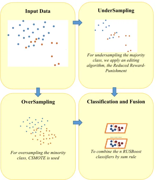
In Figure 1 we report the scheme of the proposed approach. It must be remarked that we performed several tests with other base classifiers and sampling techniques: in the end we opted for CSMOTE and RUSBoost since they work well in the maximum number of datasets (see the experiments in Section 3). The number of artificial patterns generated by CSMOTE was also set experimentally to a value that gives good results across the wider possible range of datasets.
Figure 1. Proposed approach.
Input Data UnderSampling
For undersampling the majority class, we apply an editing algorithm, the Reduced
Reward-Punishment
OverSampling
For oversampling the minority class, CSMOTE is used
Classification and Fusion
………
To combine the n RUSBoost classifiers by sum rule
13
3.1 Critical SMOTE (CSMOTE)
In this paper we introduce an improved version of MSMOTE whom we call Critical SMOTE. Following the idea of using only a subset of the minority class for building synthetic patterns, we extract from the class two prominent subsets of patterns, categorized using the method proposed in [42].
• Edge samples define the boundary of the class. These samples are enough to represent
the original data set if all classes in the data set are separated.
• Border samples are carefully selected in the overlapping region between adjacent
classes so as to obtain the best decision surface possible.
Once samples are extracted, the creation of new patterns is performed as in MSMOTE: if the
sample is of Border type, then CSMOTE randomly chooses one of the k-nearest neighbors; if it is
of Edge type, then CSMOTE selects the nearest neighbor.
4.
Experimental results
We adopt the area under the Receiver Operating Characteristic curve (AUC) [1], the F-measure [61], and the G-mean [61] as the performance measures in our experiments. The Receiver Operating Characteristic (ROC) curve is a plot of the sensitivity vs. false positive rate (1 minus specificity). The Area Under the Curve (AUC) can be interpreted as the probability that the classifier will assign a lower score to a randomly chosen positive sample rather than to a randomly chosen negative sample. The F-measure is the harmonic mean of recall and precision, and it is often used in
document retrieval. It is defined as 2 × precision × recall / (precision + recall). The G-mean is given
14 where TNrate is the specificity rate (true negative rate) and TPrate is the sensitivity rate (true
positive rate).
4.1 Tests with 2-class datasets
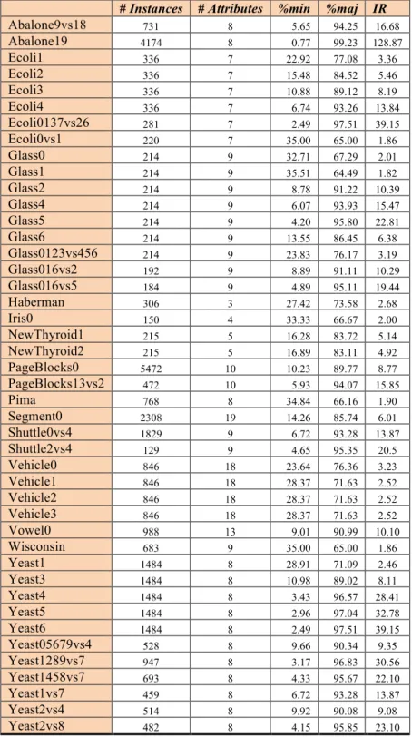
To validate our proposed approach, HardEnsemble, and compare it to existing classifiers, we resort to the same datasets tested in [3]. Table 1 summarizes the characteristics of those datasets. As in [3], a 5-fold cross-validation is adopted as the testing protocol. The folds (i.e., the dataset
partitions) are publicly available in the KEEL-dataset repository2 and serve to make a fair
comparison possible.
15
# Instances # Attributes %min %maj IR
Abalone9vs18 731 8 5.65 94.25 16.68 Abalone19 4174 8 0.77 99.23 128.87 Ecoli1 336 7 22.92 77.08 3.36 Ecoli2 336 7 15.48 84.52 5.46 Ecoli3 336 7 10.88 89.12 8.19 Ecoli4 336 7 6.74 93.26 13.84 Ecoli0137vs26 281 7 2.49 97.51 39.15 Ecoli0vs1 220 7 35.00 65.00 1.86 Glass0 214 9 32.71 67.29 2.01 Glass1 214 9 35.51 64.49 1.82 Glass2 214 9 8.78 91.22 10.39 Glass4 214 9 6.07 93.93 15.47 Glass5 214 9 4.20 95.80 22.81 Glass6 214 9 13.55 86.45 6.38 Glass0123vs456 214 9 23.83 76.17 3.19 Glass016vs2 192 9 8.89 91.11 10.29 Glass016vs5 184 9 4.89 95.11 19.44 Haberman 306 3 27.42 73.58 2.68 Iris0 150 4 33.33 66.67 2.00 NewThyroid1 215 5 16.28 83.72 5.14 NewThyroid2 215 5 16.89 83.11 4.92 PageBlocks0 5472 10 10.23 89.77 8.77 PageBlocks13vs2 472 10 5.93 94.07 15.85 Pima 768 8 34.84 66.16 1.90 Segment0 2308 19 14.26 85.74 6.01 Shuttle0vs4 1829 9 6.72 93.28 13.87 Shuttle2vs4 129 9 4.65 95.35 20.5 Vehicle0 846 18 23.64 76.36 3.23 Vehicle1 846 18 28.37 71.63 2.52 Vehicle2 846 18 28.37 71.63 2.52 Vehicle3 846 18 28.37 71.63 2.52 Vowel0 988 13 9.01 90.99 10.10 Wisconsin 683 9 35.00 65.00 1.86 Yeast1 1484 8 28.91 71.09 2.46 Yeast3 1484 8 10.98 89.02 8.11 Yeast4 1484 8 3.43 96.57 28.41 Yeast5 1484 8 2.96 97.04 32.78 Yeast6 1484 8 2.49 97.51 39.15 Yeast05679vs4 528 8 9.66 90.34 9.35 Yeast1289vs7 947 8 3.17 96.83 30.56 Yeast1458vs7 693 8 4.33 95.67 22.10 Yeast1vs7 459 8 6.72 93.28 13.87 Yeast2vs4 514 8 9.92 90.08 9.08 Yeast2vs8 482 8 4.15 95.85 23.10
Table 1. Summary description of the binary datasets used in this study.
Our first tests were performed to motivate our idea of adopting several instances of the same classifier in the ensemble. The results show that if 50 SMOTEs are combined, the fusion (by sum rule) outperforms (with p-value 0.10 using Wilcoxon signed-rank test [2]) a stand-alone
16 SMOTE. The same conclusion is also reached for RUSBoost and GK.
The use of CSMOTE instead of SMOTE or MSMOTE also deserves some motivation. CSMOTE is very useful when there are outliers in the datasets. Using the datasets reported in
Table 1 and setting the number of outliers3 to 20%, CSMOTE outperforms SMOTE with
p-value<0.01. When the number of outliers is set to 33%, CSMOTE outperforms MSMOTE as well (with p-value 0.05). When the number of outliers is limited, the three techniques perform equally well. It is important to stress in our choice of CSMOTE that a system that is robust to outliers is very important in some applications, for example, in stream data [62] or data mining in healthcare [63]. We have also tested the recent MWMOTE [60] technique using the original code shared by the authors and found that it does not outperform SMOTE (using SVM as base classifier).
After performing the first tests, we moved on to compare several different methods (including our proposed method HardEnsemble) for handling imbalanced datasets. We performed many experiments using all the methods detailed in Section 2, but here we only report the methods that performed the best in our set of experiments. The methods are listed below, and Table 2 summarizes their performance indicators:
• SVM: a plain SVM, with both the linear and the radial basis function kernel4 evaluated.
• SV_W: SVM-WEIGHT, where the parameters are overfitted using the entire dataset. We can
consider this as an upper bound of the performance that can be obtained with SVM-WEIGHT.
• CS: 50 CSMOTEs combined by sum rule, where the SVM parameters are chosen separately
using the training data in each dataset4.
• RB: 50 RUSBoosts combined by sum rule.
• B_C: fusion by sum rule of CS and RB.
3 To simulate the presence of outliers, we change the labels of a subset of the training set. 4 Its parameters are chosen, by a ten-fold cross validation using the training data, separately in each dataset.
17
• B_Cov: similar to B_C but the parameters are overfitted using the entire dataset. Again, this
gives an upper bound on the performance that can be obtained with the ensemble.
• HE_S: our proposed HardEnsemble classifier, as described in Section 3.
• HE_A: HardEnsemble, where RUSBoost is replaced by an Adaboost of 50 neural networks
as the base classifier.
• HE_FUS: fusion by sum rule5 of HE_S and HE_A.
• Best: best result (separately chosen for each dataset) as reported in [3].
The most interesting fact emerging from our tests is that no single stand-alone method (including, of course, those described in Section 2 and not listed here because of their lower
performance in the tests) outperforms SVM with p-value <0.10. Surprisingly, many surveys
(e.g., [3][4]) report the opposite result: namely, that methods for handling imbalanced datasets outperform the base classifier. In our opinion this is due to the fact that other authors use a weak base classifier (e.g., a decision tree) while we use a strong one.
18
AUC SVM SV_W CS RB B_Cov B_C HE_S HE_A HE_FUS Best
Abalone9vs18 0.9673 0.9762 0.9732 0.9583 0.9765 0.9731 0.9711 0.9661 0.9699 0.766 Abalone19 0.7252 0.7467 0.7321 0.7197 0.7659 0.7325 0.7902 0.8303 0.8338 0.720 Ecoli1 0.9597 0.9592 0.9587 0.9594 0.9646 0.9599 0.9567 0.9605 0.9607 0.919 Ecoli2 0.9648 0.9651 0.9651 0.9678 0.9698 0.9669 0.9643 0.9681 0.9701 0.908 Ecoli3 0.9513 0.9406 0.9425 0.9468 0.9597 0.9423 0.9499 0.9480 0.9511 0.907 Ecoli4 0.9978 0.9975 0.9895 0.9802 0.9986 0.9892 0.9911 0.9883 0.9901 0.941 Ecoli0137vs26 0.9567 0.9585 0.9589 0.9419 0.9622 0.9586 0.9610 0.9473 0.9588 0.848 Ecoli0vs1 0.9930 0.9927 0.9935 0.9950 0.9947 0.9936 0.9945 0.9941 0.9949 0.983 Glass0 0.8556 0.8658 0.8634 0.8675 0.8681 0.8674 0.8657 0.8593 0.8697 0.862 Glass1 0.7934 0.7954 0.7887 0.7889 0.7986 0.7872 0.7910 0.8090 0.8031 0.820 Glass2 0.8759 0.8957 0.8687 0.8856 0.8807 0.8849 0.8803 0.8545 0.8727 0.779 Glass4 0.9800 0.9704 0.9745 0.9652 0.9727 0.9631 0.9834 0.9828 0.9871 0.937 Glass5 0.9981 0.9988 0.9983 0.9852 1.0000 0.9931 0.9985 0.9986 0.9985 0.985 Glass6 0.9694 0.9218 0.9571 0.9744 0.9800 0.9681 0.9798 0.9811 0.9806 0.936 Glass0123vs456 0.9805 0.9783 0.9886 0.9827 0.9888 0.9852 0.9868 0.9881 0.9903 0.945 Glass016vs2 0.8528 0.8796 0.8233 0.8778 0.8836 0.8636 0.8601 0.8088 0.8217 0.753 Glass016vs5 0.9833 0.9976 0.9890 0.9718 0.9979 0.9896 0.9892 0.9899 0.9897 0.988 Haberman 0.7098 0.6985 0.6748 0.7043 0.7116 0.6941 0.7084 0.6975 0.7206 0.668 Iris0 1.0000 1.0000 1.0000 1.0000 1.0000 1.0000 1.0000 1.0000 1.0000 0.990 NewThyroid1 1.0000 1.0000 1.0000 0.9991 1.0000 1.0000 1.0000 0.9998 1.0000 0.988 NewThyroid2 1.0000 1.0000 1.0000 0.9981 1.0000 1.0000 0.9993 0.9993 0.9997 0.985 PageBlocks0 0.9797 0.9811 0.9804 0.9821 0.9835 0.9821 0.9812 0.9913 0.9910 0.958 PageBlocks13vs2 0.9985 0.9979 0.9997 0.9997 0.9998 1.0000 0.9982 1.0000 1.0000 0.997 Pima 0.8372 0.8306 0.8394 0.8255 0.8412 0.8399 0.8389 0.8320 0.8391 0.763 Segment0 1.0000 1.0000 1.0000 1.0000 1.0000 1.0000 1.0000 1.0000 1.0000 0.996 Shuttle0vs4 1.0000 1.0000 1.0000 1.0000 1.0000 1.0000 1.0000 1.0000 1.0000 1.000 Shuttle2vs4 1.0000 1.0000 1.0000 1.0000 1.0000 1.0000 1.0000 1.0000 1.0000 1.000 Vehicle0 0.9985 0.9986 0.9990 0.9981 0.9986 0.9995 0.9961 0.9985 0.9986 0.976 Vehicle1 0.9302 0.9385 0.9193 0.9219 0.9314 0.9192 0.9137 0.9027 0.9108 0.800 Vehicle2 0.9983 0.9987 0.9984 0.9976 0.9990 0.9984 0.9987 0.9987 0.9984 0.985 Vehicle3 0.9113 0.9175 0.9033 0.9049 0.9135 0.9031 0.8956 0.8938 0.8962 0.802 Vowel0 1.0000 1.0000 1.0000 1.0000 1.0000 1.0000 1.0000 1.0000 1.0000 0.991 Wisconsin5 0.9952 0.9952 0.9958 0.9916 0.9951 0.9959 0.9956 0.9937 0.9958 0.978 Yeast1 0.7963 0.8001 0.7964 0.8018 0.8072 0.7983 0.8033 0.7996 0.8052 0.739 Yeast3 0.9741 0.9711 0.9739 0.9709 0.9741 0.9733 0.9741 0.9744 0.9744 0.944 Yeast4 0.8796 0.8821 0.9034 0.8950 0.9092 0.9033 0.8962 0.9091 0.9096 0.860 Yeast5 0.9897 0.9904 0.9898 0.9890 0.9900 0.9905 0.9909 0.9928 0.9922 0.965 Yeast6 0.9235 0.9444 0.9434 0.9209 0.9496 0.9436 0.9461 0.9393 0.9446 0.877 Yeast05679vs4 0.8804 0.8864 0.8728 0.8816 0.8883 0.8780 0.8732 0.8816 0.8875 0.818 Yeast1289vs7 0.7666 0.8018 0.8128 0.7590 0.8235 0.8128 0.8211 0.8057 0.8122 0.733 Yeast1458vs7 0.6816 0.7096 0.6974 0.7095 0.7257 0.7116 0.7014 0.7031 0.7088 0.626 Yeast1vs7 0.7957 0.8628 0.8542 0.8155 0.8585 0.8549 0.8520 0.8491 0.8581 0.785 Yeast2vs4 0.9756 0.9809 0.9808 0.9738 0.9815 0.9803 0.9789 0.9825 0.9833 0.941 Yeast2vs8 0.8249 0.8630 0.8519 0.8342 0.8774 0.8514 0.8122 0.8255 0.8312 0.833 MeanAUC 0.9239 0.9293 0.9262 0.9237 0.9346 0.9284 0.9293 0.9283 0.9318 0.887
19
F-MEASURE SVM SV_W CS RB B_Cov B_C HE_S HE_A HE_FUS Abalone9vs18 0.5489 0.6034 0.5852 0.5011 0.6025 0.5850 0.5748 0.5426 0.5647 Abalone19 0.0562 0.0490 0.0314 0.0316 0.0448 0.0708 0.0428 0.0738 0.0762 Ecoli1 0.7460 0.7465 0.7388 0.7458 0.7794 0.7518 0.7266 0.7581 0.7493 Ecoli2 0.7694 0.7843 0.7787 0.7998 0.8206 0.7951 0.7782 0.7991 0.8140 Ecoli3 0.5409 0.4799 0.4976 0.5239 0.5952 0.4986 0.5358 0.5313 0.5444 Ecoli4 0.7664 0.7704 0.7012 0.6435 0.7707 0.7118 0.7132 0.6934 0.7103 Ecoli0137vs26 0.2931 0.2983 0.2959 0.2508 0.3104 0.2965 0.3051 0.2672 0.2955 Ecoli0vs1 0.9748 0.9705 0.9864 0.9985 0.9988 0.9872 1.0000 0.9955 0.9972 Glass0 0.5950 0.6640 0.6467 0.6654 0.6803 0.6688 0.6553 0.6172 0.6864 Glass1 0.6550 0.6609 0.6139 0.6226 0.6846 0.6098 0.6273 0.7586 0.7098 Glass2 0.4158 0.4953 0.3863 0.4556 0.4360 0.4538 0.4358 0.3287 0.4058 Glass4 0.5539 0.5002 0.5253 0.4755 0.5130 0.4616 0.5744 0.5754 0.6054 Glass5 0.8229 0.8287 0.8338 0.7209 0.8401 0.7945 0.8268 0.8335 0.8357 Glass6 0.7199 0.3309 0.6296 0.7643 0.8101 0.7191 0.8064 0.8230 0.8127 Glass0123vs456 0.8064 0.7748 0.8680 0.8208 0.8807 0.8427 0.8487 0.8736 0.8816 Glass016vs2 0.4405 0.5444 0.3279 0.5361 0.5620 0.4822 0.4689 0.2667 0.3235 Glass016vs5 0.7257 0.8365 0.7756 0.6364 0.8487 0.7814 0.7761 0.7809 0.7811 Haberman 0.4883 0.4249 0.3011 0.4556 0.4907 0.4019 0.4721 0.4161 0.5452 Iris0 1.0000 0.9949 1.0000 0.9958 1.0000 0.9958 1.0000 0.9947 0.9936 NewThyroid1 0.9574 0.9417 0.9421 0.9393 0.9454 0.9435 0.9529 0.9504 0.9519 NewThyroid2 0.9503 0.9358 0.9377 0.9349 0.9394 0.9450 0.9461 0.9315 0.9396 PageBlocks0 0.6849 0.7029 0.6848 0.6961 0.7099 0.7012 0.6919 0.7677 0.7669 PageBlocks13vs2 0.7725 0.7702 0.7922 0.7926 0.7959 0.7974 0.7817 0.7888 0.7948 Pima 0.6684 0.6153 0.6778 0.5776 0.6841 0.6804 0.6797 0.6290 0.6743 Segment0 0.9957 0.9875 0.9867 0.9923 0.9826 0.9982 0.9969 0.9891 0.9832 Shuttle0vs4 0.9934 1.0000 1.0000 1.0000 0.9972 1.0000 1.0000 0.9912 1.0000 Shuttle2vs4 0.9264 0.9255 0.9347 0.9299 0.9257 0.9287 0.9350 0.9349 0.9369 Vehicle0 0.9193 0.9262 0.9351 0.9182 0.9189 0.9374 0.9031 0.9219 0.9292 Vehicle1 0.8203 0.8796 0.7497 0.7590 0.8364 0.7433 0.6986 0.6277 0.6858 Vehicle2 0.9391 0.9468 0.9510 0.9305 0.9561 0.9374 0.9442 0.9464 0.9444 Vehicle3 0.7207 0.7618 0.6710 0.6798 0.7467 0.6625 0.6142 0.6085 0.6259 Vowel0 0.9488 0.9519 0.9527 0.9447 0.9538 0.9434 0.9470 0.9453 0.9460 Wisconsin5 0.9599 0.9607 0.9673 0.9289 0.9676 0.9643 0.9758 0.9573 0.9763 Yeast1 0.5382 0.5591 0.5328 0.5700 0.6065 0.5485 0.5755 0.5521 0.5969 Yeast3 0.6791 0.6537 0.6770 0.6630 0.6798 0.6696 0.6750 0.6801 0.6755 Yeast4 0.2410 0.2481 0.3144 0.2860 0.3372 0.3146 0.2916 0.3334 0.3364 Yeast5 0.4483 0.4500 0.4420 0.4446 0.4444 0.4457 0.4504 0.4605 0.4592 Yeast6 0.2818 0.3584 0.3488 0.2712 0.3749 0.3540 0.3640 0.3357 0.3558 Yeast05679vs4 0.4629 0.4936 0.4304 0.4744 0.5096 0.4541 0.4325 0.4706 0.5061 Yeast1289vs7 0.1224 0.2082 0.2343 0.1049 0.2595 0.2357 0.2534 0.2140 0.2340 Yeast1458vs7 0.1469 0.2033 0.1786 0.1997 0.2329 0.2054 0.1868 0.1882 0.1984 Yeast1vs7 0.1493 0.4100 0.3785 0.2248 0.3914 0.3747 0.3672 0.3517 0.3895 Yeast2vs4 0.6815 0.7192 0.7162 0.6636 0.7197 0.7161 0.6937 0.7274 0.7352 Yeast2vs8 0.6163 0.8745 0.8032 0.6831 0.9606 0.7889 0.5334 0.6208 0.6623 Mean 0.6487 0.6646 0.6537 0.6421 0.6942 0.6636 0.6604 0.6558 0.6736
20
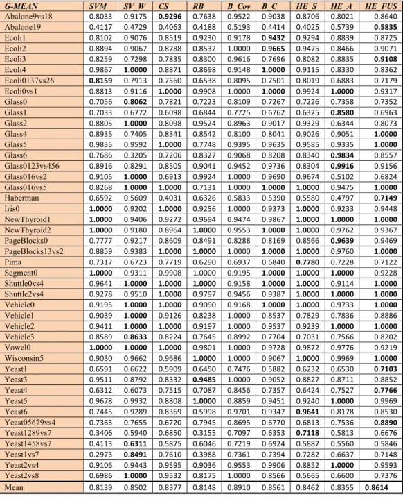
G-MEAN SVM SV_W CS RB B_Cov B_C HE_S HE_A HE_FUS
Abalone9vs18 0.8033 0.9175 0.9296 0.7638 0.9522 0.9038 0.8706 0.8021 0.8640 Abalone19 0.4117 0.4729 0.4063 0.4188 0.5193 0.4414 0.4025 0.5739 0.5835 Ecoli1 0.8102 0.9076 0.8519 0.9230 0.9178 0.9432 0.9294 0.8839 0.8725 Ecoli2 0.8894 0.9067 0.8788 0.8532 1.0000 0.9665 0.9475 0.8466 0.9071 Ecoli3 0.8259 0.7298 0.7835 0.8300 0.9616 0.7696 0.8082 0.8835 0.9108 Ecoli4 0.9867 1.0000 0.8871 0.8698 0.9148 1.0000 0.9115 0.8330 0.8362 Ecoli0137vs26 0.8159 0.7913 0.7560 0.6538 0.8095 0.7501 0.8019 0.6883 0.7179 Ecoli0vs1 0.8813 0.9116 1.0000 0.9908 1.0000 1.0000 0.9924 1.0000 0.9317 Glass0 0.7056 0.8062 0.7821 0.7223 0.8109 0.7267 0.7226 0.7358 0.7352 Glass1 0.7033 0.6772 0.6098 0.6844 0.7725 0.6762 0.6325 0.8580 0.6963 Glass2 0.8805 1.0000 0.8098 0.9524 0.8963 0.9017 0.9329 0.6344 0.8073 Glass4 0.8935 0.7405 0.8341 0.8542 0.8100 0.8041 0.9026 0.9051 1.0000 Glass5 0.9835 0.9592 1.0000 0.7748 0.9395 0.9635 0.9585 0.9335 1.0000 Glass6 0.7686 0.3205 0.7206 0.8327 0.9068 0.8208 0.8340 0.9834 0.8557 Glass0123vs456 0.8916 0.8291 0.8505 0.9041 0.9452 0.9736 0.8304 0.9916 0.9156 Glass016vs2 0.9105 1.0000 0.6913 0.9924 1.0000 0.9690 0.9674 0.5102 0.6824 Glass016vs5 0.8268 1.0000 1.0000 0.7131 1.0000 1.0000 1.0000 0.9475 1.0000 Haberman 0.6592 0.5609 0.4031 0.6326 0.5833 0.5390 0.5580 0.4797 0.7149 Iris0 1.0000 0.9202 1.0000 0.9256 1.0000 0.9373 1.0000 0.9233 0.9448 NewThyroid1 1.0000 0.9406 0.9272 0.9694 0.9474 0.9867 1.0000 1.0000 1.0000 NewThyroid2 1.0000 0.9180 0.8964 1.0000 0.9553 1.0000 1.0000 0.9762 0.9367 PageBlocks0 0.7777 0.9217 0.8609 0.8491 0.8288 0.8169 0.8566 0.9639 0.9469 PageBlocks13vs2 0.8859 0.9383 1.0000 1.0000 1.0000 1.0000 1.0000 0.9760 1.0000 Pima 0.7317 0.6723 0.7719 0.6290 0.6937 0.6840 0.7780 0.7228 0.7122 Segment0 1.0000 0.9311 0.9908 1.0000 0.9195 1.0000 1.0000 1.0000 0.9228 Shuttle0vs4 0.9641 1.0000 1.0000 1.0000 0.9158 1.0000 1.0000 0.9114 1.0000 Shuttle2vs4 0.9278 0.9510 1.0000 0.9797 0.9456 0.9387 1.0000 1.0000 1.0000 Vehicle0 0.9195 1.0000 1.0000 0.9090 0.9168 1.0000 1.0000 0.9733 1.0000 Vehicle1 0.9039 1.0000 0.9126 0.8238 1.0000 0.8537 0.7829 0.7836 0.8886 Vehicle2 0.9411 1.0000 1.0000 0.9197 1.0000 0.9537 0.9239 1.0000 1.0000 Vehicle3 0.8589 0.8633 0.8224 0.7645 0.8992 0.7704 0.7031 0.7566 0.8202 Vowel0 1.0000 1.0000 1.0000 0.9801 1.0000 0.9728 0.9872 0.9776 0.9219 Wisconsin5 0.9030 0.9662 0.9686 1.0000 1.0000 0.9067 1.0000 0.9969 1.0000 Yeast1 0.6591 0.6622 0.5909 0.6450 0.7476 0.5882 0.6232 0.6530 0.7103 Yeast3 0.9511 0.8792 0.8332 0.9485 1.0000 0.9052 0.8827 0.8711 0.8852 Yeast4 0.6312 0.6073 0.7515 0.7087 0.8456 0.7357 0.6424 0.7527 0.7766 Yeast5 0.9678 0.9932 0.8808 1.0000 0.8859 0.9451 0.9240 1.0000 0.9969 Yeast6 0.7445 0.9289 0.8369 0.5998 0.9701 0.9347 0.9641 0.8178 0.8530 Yeast05679vs4 0.7365 0.7655 0.6720 0.7945 0.8695 0.6770 0.6813 0.7536 0.8890 Yeast1289vs7 0.3406 0.5940 0.6850 0.3155 0.7097 0.6353 0.7118 0.5813 0.6676 Yeast1458vs7 0.4113 0.6311 0.5875 0.6046 0.7219 0.6924 0.5887 0.5560 0.5846 Yeast1vs7 0.2973 0.8491 0.7610 0.3988 0.7361 0.7394 0.7282 0.6637 0.7148 Yeast2vs4 0.9106 0.9443 0.9595 0.9036 0.9553 0.9906 0.8852 1.0000 0.9593 Yeast2vs8 0.6986 1.0000 0.9532 0.8175 1.0000 0.8566 0.5665 0.6600 0.7376 Mean 0.8139 0.8502 0.8377 0.8148 0.8910 0.8561 0.8462 0.8355 0.8614
Table 2. AUC, F-measure and G-mean of several classifiers and ensembles compared with the state of the art. The best performing classifier (with the exception of overfitted classifiers) for
each dataset is marked in bold.
By examining the results (considering the AUC) in Table 2, the following observations can be made.
21
• SVM is outperformed with p-value<0.05 by SVM_W, B_Cov, HE_S, and HE_FUS.
• HE_FUS outperforms B_C with p-value<0.10. The only approach that outperforms HE_FUS with p-value <0.10 is B_Cov, but it is an overfitted system that is only meaningful as an upper bound.
• The performance obtained in [3] is much lower than that obtained in this work. This is
due to the different base classifiers tested in the two papers (a decision tree in [3] vs. an SVM here). Moreover, AUC in [3] is calculated in a different way (see [3] for details).
All in all, HE_FUS is the best choice since it has no parameters6 (except the SVM
parameters in the base SVM) to be chosen for each dataset, while other approaches (e.g., SMOTE and RUSBoost) require a fine-tuning phase in order to obtain the best results. In all the tested datasets, we have used the parameters reported in Section 3.
Using the F-measure and G-mean, we have compared all the methods detailed in Section 2 and the methods reported in Table 2. Similar conclusions to those found using AUC are drawn:
in particular, HE_FUS outperforms with p-value <0.10 all the other approaches except B_Cov
(an overfitted system that is only meaningful as an upper bound). A recent paper ([66]) reports the G-mean obtained by several baseline approaches (e.g., SMOTE, Cost-sensitive SVM, SMOTEBoost, RUSBoost, SMOTEBagging, and UnderBagging) and two novel ensembles proposed by the authors of that paper. Our ensemble performs similarly to the best approaches reported in [66] and outperforms the baseline approaches. However, in all tests we always use the same parameters for building our ensembles, while in [66] the parameters are optimized for each dataset.
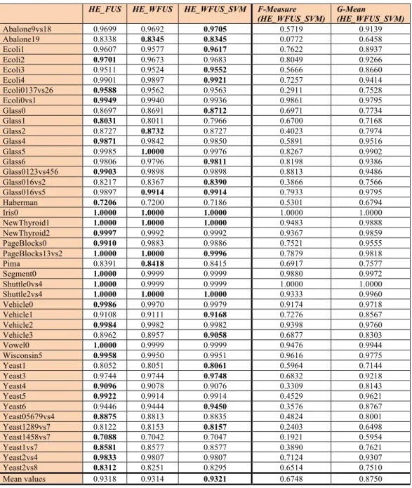
In Table 3 we report the AUC obtained by some variants of HE-FUS.
• HE_WFUS: a weighted sum rule between HE_S and HE_A where the weight of HE_S is
2 and the weight of HE_A is 1.
• HE_2WFUS: a weighted sum rule similar to HE_WFUS, but the weight of the classifiers
22 trained using the training sets built by CSMOTE is halved.
• HE_WFUS_SUM: a weighted sum rule between HE_S, HE_A, and SVM where the
weight of HE_S is 2 and the weight of HE_A and SVM is 1.
The last two columns of Table 3 report the F-measure/G-mean obtained by the best
ensemble. On average, the best results are obtained by HE_WFUS_SVM. However, there are no
statistical differences among the three ensembles.
HE_FUS HE_WFUS HE_WFUS_SVM F-Measure (HE_WFUS_SVM) G-Mean (HE_WFUS_SVM) Abalone9vs18 0.9699 0.9692 0.9705 0.5719 0.9139 Abalone19 0.8338 0.8345 0.8345 0.0772 0.6458 Ecoli1 0.9607 0.9577 0.9617 0.7622 0.8937 Ecoli2 0.9701 0.9673 0.9683 0.8049 0.9266 Ecoli3 0.9511 0.9524 0.9552 0.5666 0.8660 Ecoli4 0.9901 0.9897 0.9921 0.7257 0.9414 Ecoli0137vs26 0.9588 0.9562 0.9563 0.2911 0.7528 Ecoli0vs1 0.9949 0.9940 0.9936 0.9861 0.9795 Glass0 0.8697 0.8691 0.8712 0.6971 0.7734 Glass1 0.8031 0.8011 0.7966 0.6700 0.7168 Glass2 0.8727 0.8732 0.8727 0.4023 0.7974 Glass4 0.9871 0.9842 0.9850 0.5891 0.9516 Glass5 0.9985 1.0000 0.9976 0.8267 0.9902 Glass6 0.9806 0.9796 0.9811 0.8198 0.9386 Glass0123vs456 0.9903 0.9898 0.9898 0.8813 0.9486 Glass016vs2 0.8217 0.8367 0.8390 0.3866 0.7566 Glass016vs5 0.9897 0.9914 0.9914 0.7933 0.9795 Haberman 0.7206 0.7200 0.7186 0.5301 0.6794 Iris0 1.0000 1.0000 1.0000 1.0000 1.0000 NewThyroid1 1.0000 1.0000 1.0000 0.9483 0.9888 NewThyroid2 0.9997 0.9992 0.9992 0.9367 0.9859 PageBlocks0 0.9910 0.9883 0.9886 0.7521 0.9555 PageBlocks13vs2 1.0000 1.0000 0.9996 0.7879 0.9818 Pima 0.8391 0.8418 0.8415 0.6917 0.7577 Segment0 1.0000 0.9999 0.9999 0.9880 0.9972 Shuttle0vs4 1.0000 0.9999 0.9999 1.0000 1.0000 Shuttle2vs4 1.0000 1.0000 1.0000 0.9333 0.9960 Vehicle0 0.9986 0.9970 0.9979 0.9174 0.9718 Vehicle1 0.9108 0.9111 0.9168 0.7276 0.8567 Vehicle2 0.9984 0.9982 0.9982 0.9398 0.9760 Vehicle3 0.8962 0.8957 0.9058 0.6877 0.8303 Vowel0 1.0000 0.9999 0.9999 0.9476 0.9944 Wisconsin5 0.9958 0.9950 0.9951 0.9616 0.9775 Yeast1 0.8052 0.8051 0.8061 0.5964 0.7144 Yeast3 0.9744 0.9744 0.9748 0.6832 0.9218 Yeast4 0.9096 0.9078 0.9076 0.3309 0.8143 Yeast5 0.9922 0.9914 0.9914 0.4529 0.9621 Yeast6 0.9446 0.9444 0.9450 0.3576 0.8767 Yeast05679vs4 0.8875 0.8813 0.8835 0.4824 0.8001 Yeast1289vs7 0.8122 0.8153 0.8157 0.2403 0.6498 Yeast1458vs7 0.7088 0.7042 0.7047 0.1921 0.5954 Yeast1vs7 0.8581 0.8577 0.8577 0.3890 0.7621 Yeast2vs4 0.9833 0.9807 0.9807 0.7124 0.9307 Yeast2vs8 0.8312 0.8251 0.8295 0.6514 0.7510 Mean values 0.9318 0.9314 0.9321 0.6748 0.8750
23 In Table 4 we compare among them the methods tested in this paper (using the datasets tested in the previous table 3). Three symbols are used in the table:
• “L” indicates that the method indicated in the row exhibits lower performance, with p-value
<0.10, than the method in the column (it is the “loser”);
• “ND” indicates that there is no statistically significant difference between the performances
of the two methods;
• “W” marks the fact that the method in the row obtains higher performance, with p-value
<0.10 (it is the “winner”).
The approaches that never lose when combined with the other approaches are GK, CSMOTE, RUSBoost, and IRUS. The performances of these methods are very similar, and our ensemble outperforms them with p-value <0.10.
APLSC OCSVM GK MSMOTE CSMOTE RUSBoost EasyEnsemble BalanceCascade IRUS OverBagging UO
APLSC -‐-‐-‐-‐-‐ W L L L L L L L L L OCSVM -‐-‐-‐-‐-‐ -‐-‐-‐-‐-‐ L L L L L L L L L GK -‐-‐-‐-‐-‐ -‐-‐-‐-‐-‐ -‐-‐-‐-‐-‐ W ND ND W W ND W W MSMOTE -‐-‐-‐-‐-‐ -‐-‐-‐-‐-‐ -‐-‐-‐-‐-‐ -‐-‐-‐-‐-‐ L L ND W ND W ND CSMOTE -‐-‐-‐-‐-‐ -‐-‐-‐-‐-‐ -‐-‐-‐-‐-‐ -‐-‐-‐-‐-‐ -‐-‐-‐-‐-‐ ND W W ND W W RUSBoost -‐-‐-‐-‐-‐ -‐-‐-‐-‐-‐ -‐-‐-‐-‐-‐ -‐-‐-‐-‐-‐ -‐-‐-‐-‐-‐ -‐-‐-‐-‐-‐ W W ND W W EasyEnsemble -‐-‐-‐-‐-‐ -‐-‐-‐-‐-‐ -‐-‐-‐-‐-‐ -‐-‐-‐-‐-‐ -‐-‐-‐-‐-‐ -‐-‐-‐-‐-‐ -‐-‐-‐-‐-‐ W L ND ND BalanceCascade -‐-‐-‐-‐-‐ -‐-‐-‐-‐-‐ -‐-‐-‐-‐-‐ -‐-‐-‐-‐-‐ -‐-‐-‐-‐-‐ -‐-‐-‐-‐-‐ -‐-‐-‐-‐-‐ -‐-‐-‐-‐-‐ L L L IRUS -‐-‐-‐-‐-‐ -‐-‐-‐-‐-‐ -‐-‐-‐-‐-‐ -‐-‐-‐-‐-‐ -‐-‐-‐-‐-‐ -‐-‐-‐-‐-‐ -‐-‐-‐-‐-‐ -‐-‐-‐-‐-‐ -‐-‐-‐-‐-‐ ND ND OverBagging -‐-‐-‐-‐-‐ -‐-‐-‐-‐-‐ -‐-‐-‐-‐-‐ -‐-‐-‐-‐-‐ -‐-‐-‐-‐-‐ -‐-‐-‐-‐-‐ -‐-‐-‐-‐-‐ -‐-‐-‐-‐-‐ -‐-‐-‐-‐-‐ -‐-‐-‐-‐-‐ ND
Table 4. Comparisons (using AUC as performance indicator) between all the pairs of tested
methods.
In the previous tests, we simply combined by sum rule all the classifiers that build up our proposed system HardEnsemble. We also investigated the following alternative rules for improving the performance of the fusion step: Knora [45], MPOEC [46], SparseEnsemble [47], stacking with PCA [48], combination with correspondence analysis [49], and weighted sum rule [45]. Obviously, all the parameters for the aforementioned methods were selected using only the training data. However, no combination method outperforms the simple sum rule, with p-value <0.05.
24 To shed light on the reasons behind the good performance of the proposed ensemble, we performed experiments to measure the diversity among the decisions produced by the components of the ensemble. As already pointed out by Kuncheva [57], “there is no gain in combining identical components and, therefore, diversity is an important issue to take into consideration when designing ensemble models.” We investigated the relationship among the different components of the
ensemble by evaluating the average Yule’s Q-statistic [57]over the datasets detailed in Table 1. For
two classifiers Gi and Gj, the Q-statistic is an a posteriori measure defined as:
10 01 00 11 10 01 00 11 , N N N N N N N N Qi j + − =
where Nab is the number of instances in the testing set that are classified correctly (a=1) or
incorrectly (a=0) by classifier Gi and correctly (b=1) or incorrectly (b=0) by the classifier Gj. Qi,j
varies between –1 and 1 and assumes the value 0 for statistically independent classifiers. Classifiers
that tend to recognize the same patterns correctly will have Q>0, and those that commit errors on
different patterns will have Q<0.
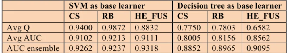
In Table 5 we report the Q-statistic among the classifiers that compose CS, RB, and HE_FUS (see Section 4.1 for the description of these ensemble classifiers). In the same table we also report
the performance of modified ensembles where a decision tree, implemented as in http://prtools.org/,
is used as the base learner instead of SVM. Such modified ensembles exhibit a low Q-statistic; indeed, the average performance of the base learner is so low that the ensembles coupled with SVM outperform the ensembles based on decision trees. Ensembles of SVMs have already been proposed in the literature [68-69]. All in all, for each ensemble we report:
• “Avg Q”, the average Q-statistic among the classifiers of the given ensemble;
• “Avg AUC”, the average AUC obtained by the classifiers of the given ensemble;
25
SVM as base learner Decision tree as base learner
CS RB HE_FUS CS RB HE_FUS
Avg Q 0.9400 0.9872 0.8832 0.7750 0.7803 0.6582 Avg AUC 0.9102 0.9213 0.9111 0.8005 0.8156 0.8562 AUC ensemble 0.9262 0.9237 0.9318 0.8852 0.8965 0.9095
Table 5. Yule’s Q-statistic among the classifiers forming the different ensembles.
The reported results in Table 5 experimentally endorse our idea of building an ensemble where two different classifiers are employed and where two different methods are used for creating the different training sets. The Q-statistic among the classifiers of HE_FUS is quite low, and lower than that obtained by an ensemble of RUSBoosts or SMOTEs. The low Q-statistic boosts the performance obtained by the single classifiers that contribute to HE_FUS.
4.2 Tests with multi-class datasets
We now shift focus to multi-class datasets in order to test the validity of our approach in this domain as well. We consider the multi-class datasets tested in [4]. The data partitions are, again, available in the KEEL-dataset repository, so it is still possible to report a fair comparison. The methods are applied to the original multi-class data directly. As in [4], we adopt the extension of AUC for multi-class datasets as the performance indicator. This extension is called MAUC [54], and it represents the average AUC of all pairs of classes. The results of our tests are summarized in
Table 6. The column Best reports the best result, separately chosen for each dataset, among the
methods proposed in [4]. In Table 6 we also report the performance of what in [4]is considered the
best approach, i.e., SMB-dw. Since SVM is a 2-class classifier we use the one-vs-all approach for handling multiclass classification.
26
Table 6. Performance (MAUC) in the multi-class datasets.
The following conclusions can be drawn from Table 6.
• As in the previous comparison, the performance of the method based on decision trees, i.e.,
SMB-dw, is often lower than that obtained with a plain SVM.
• HE_S performs similarly to SVM, but HE_FUS outperforms SVM. This is further
experimental evidence that the heterogeneous ensemble approach is a sound approach method for handling imbalanced datasets.
4.3 Tests with strongly imbalanced datasets
In this series of tests, the 5-fold cross-validation testing protocol is used in what we consider to be strongly imbalanced 2-class datasets. Some of these datasets are retrieved from the UCI Machine Learning Repository:
• PIMA: the Pima Indians diabetes dataset;
• IONO:the Ionosphere dataset;
• CreditG: the German credit data dataset;
• Sonar: Mines vs. Rocks dataset;
• Breast: the Breast cancer dataset;
SMB-dw
[4]
Best SVM HE_S HE_A HE_FUS
Car 0.997 0.997 0.9913 0.9876 0.9903 0.9925 Balance 0.633 0.703 0.9992 0.9965 0.9906 0.9944 Glass 0.924 0.925 0.9486 0.9649 0.9625 0.9687 New-Thyroid 0.988 0.988 0.9991 0.9994 0.9991 0.9994 PageBlocks 0.973 0.989 0.9696 0.9825 0.9821 0.9908 Yeast 0.847 0.857 0.9256 0.9282 0.9332 0.9348
27
• Yeast: the Yeast UCI dataset where only the classes ‘POX’ and ‘CYT’ are considered (as in
[37]);
• Wdbc: the Cancer Wisconsin Diagnostic Data Set;
• Wpbc: the Wisconsin Prognostic Breast Cancer;
• House: the Housing Data Set;
• Haber: the Haberman's Survival Data Set;
• Transf: the Blood Transfusion Service Center;
• Austr: the Australian Credit Approval Data Set.
Other datasets used in the following tests include Astro (the astronomical matching catalogues
in [67]) and spot (the microarray spot quality classification dataset in [70]).
For all datasets (except CreditG and Yeast), we randomly keep only ten patterns of the minority class, with the aim of increasing the imbalance. For reproducible research, the specific datasets used in these tests (i.e. the split training/testing sets and the randomly selected patterns) will be available with the software tool created for this paper.
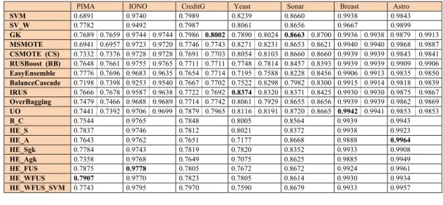
Results of the tests are summarized in Table 7. For some methods, two values are reported: the first one is for a “standard” execution of the method, while the second one gives the performance obtained with 50 executions combined with the sum rule. Notice that in this test, GK and other approaches work better than SVM; this is not the case with the datasets reported in Table 1 (here the datasets are strongly imbalanced). In the last column of Table 7, the average performance over several datasets is reported.
We also ran another experiment changing CSMOTE with GK in our ensemble (see HE_Sgk and HE_Agk), without obtaining any improvement.
The same conclusion in the previous tests is obtained here: the ensemble works quite well in all the tested datasets.
28
PIMA IONO CreditG Yeast Sonar Breast Astro
SVM 0.6891 0.9740 0.7989 0.8239 0.8660 0.9938 0.9843 SV_W 0.7782 0.9492 0.7987 0.8061 0.8656 0.9667 0.9899 GK 0.7689 0.7659 0.9744 0.9744 0.7986 0.8002 0.7890 0.8024 0.8663 0.8700 0.9936 0.9938 0.9879 0.9913 MSMOTE 0.6941 0.6957 0.9723 0.9720 0.7746 0.7743 0.8271 0.8231 0.8653 0.8621 0.9940 0.9940 0.9868 0.9887 CSMOTE (CS) 0.7332 0.7376 0.9728 0.9728 0.7691 0.7703 0.8054 0.8103 0.8660 0.8660 0.9939 0.9939 0.9843 0.9841 RUSBoost (RB) 0.7648 0.7661 0.9755 0.9765 0.7711 0.7711 0.7748 0.7814 0.8457 0.8393 0.9939 0.9939 0.9909 0.9906 EasyEnsemble 0.7776 0.7696 0.9683 0.9635 0.7654 0.7714 0.7195 0.7588 0.8228 0.8456 0.9906 0.9913 0.9835 0.9850 BalanceCascade 0.7198 0.7398 0.9253 0.9540 0.7667 0.7702 0.7522 0.8298 0.7982 0.8300 0.9915 0.9914 0.9818 0.9839 IRUS 0.7666 0.7678 0.9587 0.9638 0.7722 0.7692 0.8374 0.8320 0.8371 0.8425 0.9930 0.9930 0.9875 0.9867 OverBagging 0.7479 0.7466 0.9688 0.9689 0.7714 0.7742 0.8061 0.7929 0.8655 0.8656 0.9939 0.9939 0.9862 0.9869 UO 0.7441 0.7392 0.9706 0.9699 0.7879 0.7965 0.8116 0.8191 0.8720 0.8665 0.9942 0.9941 0.9853 0.9853 B_C 0.7544 0.9765 0.7848 0.8005 0.8564 0.9939 0.9943 HE_S 0.7837 0.9746 0.7812 0.8021 0.8372 0.9938 0.9923 HE_A 0.7643 0.9762 0.7651 0.7177 0.8668 0.9888 0.9964 HE_Sgk 0.7784 0.9743 0.7819 0.7820 0.8352 0.9933 0.9908 HE_Agk 0.7358 0.9768 0.7649 0.7075 0.8625 0.9885 0.9949 HE_FUS 0.7875 0.9778 0.7805 0.7672 0.8672 0.9924 0.9961 HE_WFUS 0.7907 0.9770 0.7823 0.7805 0.8614 0.9930 0.9934 HE_WFUS_SVM 0.7743 0.9795 0.7970 0.7590 0.8679 0.9933 0.9957
wdbc spot wpbc House Haber Transf Austr AVG
SVM 0.9929 0.9479 0.5765 0.9731 0.6281 0.5654 0.8502 0.8331 SV_W 0.9851 0.9479 0.5937 0.9731 0.6814 0.7059 0.8453 0.8491 GK 0.9930 0.9929 0.9637 0.9598 0.6044 0.5981 0.9769 0.9768 0.6950 0.6930 0.6418 0.6454 0.8886 0.8883 0.8530 0.8537 MSMOTE 0.9902 0.9901 0.9618 0.9579 0.6055 0.6090 0.9680 0.9677 0.6671 0.6689 0.6181 0.6167 0.8282 0.8276 0.8395 0.8391 CSMOTE (CS) 0.9929 0.9928 0.9536 0.9685 0.5765 0.5765 0.9675 0.9703 0.6281 0.6281 0.5654 0.5654 0.8502 0.8502 0.8328 0.8348 RUSBoost (RB) 0.9913 0.9910 0.9565 0.9615 0.5999 0.5980 0.9779 0.9792 0.6996 0.6960 0.6297 0.6297 0.8902 0.8927 0.8473 0.8476 EasyEnsemble 0.9729 0.9760 0.9572 0.9633 0.5858 0.6143 0.9748 0.9761 0.6386 0.6510 0.6394 0.6420 0.8753 0.8938 0.8337 0.8430 BalanceCascade 0.9681 0.9743 0.9502 0.9642 0.5964 0.5965 0.9773 0.9754 0.6199 0.6439 0.6309 0.5217 0.8809 0.8928 0.8257 0.8334 IRUS 0.9841 0.9840 0.9698 0.9619 0.6004 0.5980 0.9766 0.9779 0.6851 0.6826 0.7103 0.7119 0.8953 0.8958 0.8550 0.8549 OverBagging 0.9908 0.9910 0.9504 0.9479 0.5962 0.6021 0.9731 0.9731 0.6933 0.6831 0.6393 0.6399 0.8560 0.8581 0.8456 0.8446 UO 0.9896 0.9892 0.9447 0.9418 0.6100 0.6151 0.9731 0.9731 0.6829 0.6875 0.6883 0.6937 0.8552 0.8552 0.8507 0.8519 B_C 0.9922 0.9699 0.5936 0.9761 0.6742 0.6222 0.8885 0.8484 HE_S 0.9889 0.9663 0.6020 0.9821 0.6925 0.6596 0.8981 0.8539 HE_A 0.9858 0.9803 0.5808 0.9849 0.6487 0.6638 0.8927 0.8437 HE_Sgk 0.9885 0.9620 0.6024 0.9832 0.6891 0.6532 0.8895 0.8503 HE_Agk 0.9864 0.9790 0.5882 0.9851 0.6558 0.6435 0.8785 0.8391 HE_FUS 0.9895 0.9787 0.6015 0.9851 0.6776 0.6753 0.9002 0.8555 HE_WFUS 0.9906 0.9755 0.6020 0.9844 0.6866 0.6773 0.9008 0.8568 HE_WFUS_SVM 0.9918 0.9715 0.6015 0.9838 0.6809 0.6717 0.8992 0.8548
Table 7. Results (AUC) in strongly imbalanced datasets. A number of conclusions can be drawn from the results in Table 7.
• In some datasets (PIMA, ASTRO, Spot, Wpbc, Haber, and Tranf/Austr), SVM performs
quite poorly with respect to the best approaches for handling imbalance, while it works well with the other datasets.
• Our proposed ensembles HE_FUS and HE_WFUS exhibit good results across all the
datasets except Yeast, where they are outperformed by several methods. However, notice