Contextual Bag-Of-Visual-Words and
ECOC-Rank for Retrieval and Multi-class
Object Recognition
Mehdi Mirza-Mohammadi
Dept. Matem`atica Aplicada i An`alisi, Universitat de Barcelona, Gran Via 585, 08007, Barcelona, Spain. E-mail: [email protected]
Abstract
Multi-class object categorization is an important line of research in Computer Vision and Pattern Recognition fields. An artificial intelligent system is able to interact with its environment if it is able to distinguish among a set of cases, instances, situations, objects, etc. The World is inherently multi-class, and thus, the efficiency of a system can be determined by its accuracy discriminating among a set of cases. A recently applied procedure in the literature is the Bag-Of-Visual-Words (BOVW). This methodology is based on the natural language processing theory, where a set of sentences are defined based on word frequencies. Analogy, in the pattern recognition domain, an object is described based on the frequency of its parts appearance. However, a general drawback of this method is that the dictionary construction does not take into account geometrical information about object parts. In order to include parts relations in the BOVW model, we propose the Contextual BOVW (C-BOVW), where the dictionary construction is guided by a geometricaly-based merging procedure. As a result, objects are described as sentences where geometrical information is implicitly considered.
In order to extend the proposed system to the multi-class case, we used the Error-Correcting Output Codes framework (ECOC). State-of-the-art multi-class techniques are frequently defined as an ensemble of binary classifiers. In this sense, the ECOC framework, based on error-correcting principles, showed to be a powerful tool, being able to classify a huge number of classes at the same time that corrects classification errors produced by the individual learners.
In our case, the C-BOVW sentences are learnt by means of an ECOC configu-ration, obtaining high discriminative power. Moreover, we used the ECOC outputs obtained by the new methodology to rank classes. In some situations, more than one label is required to work with multiple hypothesis and find similar cases, such as in the well-known retrieval problems. In this sense, we also included contextual and semantic information to modify the ECOC outputs and defined an ECOC-rank methodology. Altering the ECOC output values by means of the adjacency of classes based on features and classes relations based on ontologies, we also reported a significant improvement in class-retrieval problems.
Resum
La multi-classificaci´o d’objectes ´es una important l´ınia de investigaci´o a les `arees de Visi´o Artificial i Reconeixement de Patrons. Un sistema intel·ligent ´es capa¸c de interactuar amb el seu entorn si pot distingir entre un conjunt de casos, inst`ancies, situacions, objectes, etc. El m´on ´es inherentment multi-classe. i per tant, la efic`acia d’un sistema pot estar determinada por la seva robustesa discriminant entre un conjunt de casos. Un m`etode recent en aquest `ambit ´es el ”Bag-of-Visual-Words” (BOVW). Aquesta metodologia es basa en el processament del llenguatge natural, on un conjunt de sent`encies es defineixen en funci´o de la freq¨u`encia de les seves paraules. De forma an`aloga, en el domini del Reconeixement de Patrons, un objecte ´es descrit a partir de la freq¨u`encia d’aparici´o de les parts que el composen. No obstant, un dels principals problemes d’aquesta metodologia ´es que la construcci´o del diccionari no t´e en compte la informaci´o geom`etrica entre les parts dels objectes. Amb l’objectiu d’incloure informaci´o relacional entre les parts dels objectes, en aquest treball proposem el BOVW contextual (C-BOVW), on la construcci´o del diccionari b´e guiada per un proc´es de fusi´o. Com a resultat, els objectes s´on descrits com sent`encies a on la informaci´o geom`etrica est`a impl´ıcitament definida.
Amb l’objectiu d’estendre el sistema proposat al cas multi-classe, hem utilitzat el marc dels ”Error-Correcting Output Codes” (ECOC). Les t`ecniques de multi-classificaci´o de l’estat de l’art freq¨uentment estan definides a partir de l’assemblatge de classificadors binaris. En aquest sentit, el marc dels ECOC, basats en els principis de la correcci´o d’errors, han demostrar ser una potent eina, essent capa¸cos de clas-sificar grans conjunts de classes a la vegada que corregeixen errors de classificaci´o produ¨ıts pels classificadors individuals.
En el nostre cas, les sent`encies C-BOVW s´on apreses per mitj`a d’un disseny ECOC. obtenint un alt poder discriminador. A m´es, hem considerat les sortides dels ECOC amb l’objectiu d’ordenar i obtenir un ranking de les classes. En al-gunes situacions, m´es d’una etiqueta ´es necess`aria amb l’objectiu de treballar amb m´ultiples hip`otesis i trobar casos similars, com ´es el cas dels ben coneguts problemes de ”retrieval”. En aquest sentit, hem incl`os informaci´o contextual i sem`antica per modificar les sortides dels ECOC i definir la metodologia ECOC-Rank. Alterant les sortides dels ECOC a partir de l’adjac`encia entre classes basada en valors de carac-ter´ıstiques i les relacions entre classes per mitj`a d’ontologies, tamb´e hem obtingut millores significatives en els problemes de ”retrieval” de classes.
Resumen
La multi-clasificaci´on de objetos en una importante l´ınea de investigaci´on en las ´areas de Visi´on Artificial y Reconocimiento de Patrones. Un sistema inteligente es capaz de interactuar con su entorno en la medida que pueda distinguir entre un conjunto de casos, instancias, situaciones, objetos, etc. El mundo es inherente-mente multi-clase, y por lo tanto, la eficacia de un sistema puede venir determinada por su robustez discriminando entre un conjunto de casos. Un m´etodo reciente en este ´ambito ampliamente considerado en la literatura es el ”Bag-of-Visual-Words” (BOVW). Esta metodolog´ıa se basa en el procesamiento del lenguaje natural, donde un conjunto de frases se definen en funci´on de la frecuencia de aparici´on de sus pal-abras. De forma an´aloga, en el dominio del Reconocimiento de Patrones, un objeto es descrito a partir de la frecuencia de aparici´on de las partes que lo componen. No ob-stante, uno de los problemas principales de esta metodolog´ıa es que la construcci´on del diccionario no tiene en cuenta la informaci´on geom´etrica entre las partes de los objetos. Con el objetivo de incluir informaci´on relacional entre las partes de los objetos, en este trabajo proponemos el BOVW contextual (C-BOVW), donde la construcci´on del diccionario viene determinada por un proceso guiado de mezcla. Como resultado, los objetos son descritos como sentencias donde la informaci´on geom´etrica est´a impl´ıcitamente definida.
Con el objetivo de extender el sistema propuesto al caso multi-clase, hemos us-ado el marco de los ”Error-Correcting Output Codes” (ECOC). Las t´ecnicas de multi-clasificaci´on del estado del arte frecuentemente vienen definidas a trav´es del ensamblaje de clasificadores binarios. En este sentido, el marco de los ECOC, basa-dos en los principios de correcci´on de errores, han demostrado ser una potente herramienta, siendo capaces de clasificar grandes conjuntos de clases a la vez que corrijen errores de clasificaci´on producidos por los clasificadores individuales.
En nuestro caso, las sentencias C-BOVW son aprendidas a trav´es de un dise˜no ECOC, obteniendo un alto poder de discriminaci´on. Adem´as, hemos considerado las salidas de los ECOC con el objetivo de ordenar y obtener un ranking de las clases. En algunas situaciones, m´as de una etiqueta es necesaria con el objetivo de trabajar con m´ultiples hip´otesis y encontrar casos similares o candidatos, como en los bien conocidos problemas de ”retrieval”. En este sentido, hemos incluido informaci´on contextual y sem´antica para modificar las salidas de los ECOC y definir la metodolog´ıa ECOC-Rank. Alterando las salidas de los ECOC a trav´es de la adyacencia de clases basada en valores de caracter´ısticas y las relaciones entre clases bas´andonos en ontolog´ıas, tambi´en hemos obtenido mejoras significativas en los problemas de ”retrieval” de clases.
Key words: Multi-class classification, Bag-Of-Visual Words, Error-Correcting Output Codes, Retrieval, Ranking.
Acknowledgements
I like to give my special thanks to my advisor Sergio Escalera, who taught me in the research and helped me through each step of my study. Also I like to thanks Oriol Pujol and Petia Padeva for their help and supervision through my study at UB and all other colleagues and friends there.
1 Introduction
We, humans from our first days of life learn to group our observations into meaningful and abstract categories. We can learn new categories from just few instances, and have the ability to recognize any new instance easily. As a matter of fact, categorization is the most fundamental cognitive ability, which helps us get through daily life.
For computers, images are just array of data, and machine has no knowledge about its semantic meaning. Categorization is one of the most challenging tasks in computer vision, which could have plenty of applications.
The task of object categorization in computer vision usually is split in two main stages: object description, where discriminative features are extracted from the object to represent, and object classification, where a set of extracted features are labeled as a particular object given the output of a trained clas-sifier. There are plenty of methods on feature extraction, which vary based on the application, like localizing and classifying single objects, texture, or scenes. Recognition of real world scenes may be initiated from the global con-figuration, ignoring most of the details and object information (Bidderman, 1988; Potter, 1976) [1], meanwhile in object recognition the main attention is focused on the characteristic of individual instances. An example of an object categorization task is shown in Figure 1. In the image, the Wall-E robot of the Disney’s film categorizes new objects into a set of categories.
A general tendency in object recognition to deal with the object description stage is to define a bottom-up procedure where initial features are obtained by means of region detection techniques. These techniques are based on de-termining relevant image key-points (i.e. using edge-based information [2]), and then defining a support region around the key-point (i.e. looking for ex-trema over scale-space [2]). Several alternatives for region detection have been proposed in the literature [2]. Once a set of regions is defined, it should be described using some kind of descriptor (i.e. SIFT descriptor [3]), and the region-descriptions are related in some way to define a model of the object of interest. Very few methods take into account relations of object parts when defining the feature space, such as in the Shape Context descriptor [4], and relations use to take place in the learning step, such as in graphical models as Conditional Random Fields or Hidden Markov Models [5,6].
1.1 Contextual Bag-of-Visual-Words motivation
Based on the previous tendency, a recent technique to model visual objects is by means of a Bag-Of-Visual-Words. The BOVW model is inspired by the text
Fig. 1. Scene of the Disney’s Wall-e film. From top to down and left to right: The robot classifies objects into different categories. For a new object, the robot considers two classification options, fork and spoon. Finally, he classifies the new object in a new Fork-Spoon category.
classification problem using a Bag-Of-Words. In Bag-Of-Words model each document is represented by an unsorted set of contained words, regardless of the grammar and word order, and assumes order of words has no significance. Analogously, in object categorization problems, an image is represented by an unsorted set of discrete visual words, which are obtained by the object local descriptions.
Many promising results have been achieved with the BOVW systems in natu-ral language processing, texture recognition, Hierarchical Bayesian models for documents, object classification [7], object retrieval problems [8,9], or natural scene categorization [10], just to mention a few. However, one of the main drawbacks of the BOVW model is that dictionary construction does not take into account the geometrical information among visual instances. Although this issue can be beneficial in natural language analysis, its adaptation to visual word description needs special attention. Note that based on the de-scription strategy used to describe visual words, very close regions can have far descriptors in the feature space, being grouped as different visual words. This effect occurs for most of the state-of-the-art descriptors, even when coping with different invariance, and thus, a grouping based on spatial information of regions could be beneficial for the construction of the visual dictionary.
in-formation of visual words in the dictionary construction step, which we call Contextual Bag-Of-Visual-Words model. Objects interest regions are obtained by means of the Harris-Affine detector and then described using the SIFT de-scriptor. Afterward, a contextual-space and a feature-space are defined. The first space codifies the contextual properties of regions meanwhile the second space contains the region descriptions. A merging process is then used to fuse feature words based on their proximity in the contextual-space. Moreover, the new dictionary is learned using the Error Correcting Output Codes frame-work [11] in order to perform multi-class object categorization. We compared our approach to the standard BOVW design and validated over public multi-class categorization data sets, considering different state-of-the-art multi-classifiers in the ECOC multi-classification procedure. Results show significant classi-fication improvements when spatial information is taken into account in the dictionary construction step.
On the other hand, we extended our methodology to deal with another chal-lenging computer vision task. In many situations only one predicted label of a multi-class problem is not enough, and we need to retrieve several possible and ordered case. This is the case of the retrieval problem.
1.2 ECOC-Rank motivation
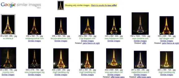
Information Retrieval deals with uncertainty and vagueness in information systems (IR Specialist Group of German Informatics Society, 1991). This in-formation could be in forms such as text, audio, or image. The science field which deals with information retrieval in images which is called Content-based image retrieval (CBIR). CBIR corresponds to any technology that for example helps to organize digital picture archives by their visual content. By this defi-nition, anything ranging from an image similarity function to a robust image annotation engine falls under the purview of CBIR [12]. An example of a real image retrieval system is shown in Figure 2, where a set of Tour Eiffel samples are retrieved given an input sample using the Google retrieval engine.
In last decade, many research and work have been performed to describe color, shape, and texture features, without considering image semantics. Eakins [13] defines three levels of queries in CBIR.
Level 1: Retrieval by primitive features such as color, texture, shape, or the spatial location of image elements. A typical query is for example ’find pictures like this’.
Level 2: Retrieval of objects of a given type identified by derived features, considering some degree of logical inference. For example ’find a picture of a flower’.
Level 3: Retrieval by abstract attributes, involving a significant amount of high-level reasoning about the purpose of the objects or scenes depicted. This includes retrieval of named events, pictures with emotional or religious signif-icance, etc. A query example could be ’find pictures of a joyful crowd’.
Levels 2 and 3 together are referred to as semantic image retrieval, and the gap between Levels 1 and 2 as the semantic gap [13]. Recently, some research has focused to fill this gap. Some state-of-the-art techniques use object ontology to define high-level concepts [14–17]. Other works use supervised or unsupervised learning methods to associate low-level features with query concepts [18–22], introduce Relevance feedback into retrieval loop for continuous learning of users intention [23–25], generate Semantic Template to support high-level im-age retrieval [26–28], or make use of both textual information obtained from the Web and visual content of images for Web image retrieval [29,27,30]. Many systems exploit one or more of the above techniques to implement high-level semantic-based image retrieval [23,24,27,30,20,29,27,31].
Fig. 2. Example of the retrieval of similar images for a Eiffel tower sample using the Google Similar Images engine (http://similar-images.googlelabs.com/). In this case, the retrieval process is based on a graph of relations designed by means of image features and web links.
Most of the works in the literature related to retrieval processes are based on the retrieving of samples from a same category. However, in our case we based on the class retrieval problem. Here, we define the class retrieval problem as the problem of retrieving classes similar in some way (i.e. given a semantic class distance) to the original class label of a given sample. Suppose we have an image from a cat animal category. In that case, we want to retrieve similar categories and not just samples from the same animal (i.e. tiger could be a possible solution). In order to deal with this problem, we focus on the output of multi-class classifiers to rank classes and then perform class retrieval.
learn-ing binary functions [32,33], but in many real-world learnlearn-ing tasks, such as in object classification, we need to deal with a discrete set of classes. Some of the state-of-the-art binary classification methods have been extended to deal with multi-class problems, such as decision trees, Adaboost, and Support Vector Machines. However, this kind of extensions is not always trivial. In such cases, the usual way to proceed is to reduce the complexity of the problem to a set of simpler classifiers and to combine them. In this sense, Error-Correcting output code (ECOC) is a general framework that combines binary problems to address the multi-class problem. The ECOC technique can be broken into two stages, encoding and decoding. Given a set of classes, the coding stage designs a codeword for each class based on different binary problems. The decoding stage makes a classification decision for a given test sample based on the value of the output code. Based on error-correcting properties, the ECOC framework has shown to be a powerful tool for combining binary classifiers, outperforming classical voting procedures.
Up to now, the ECOC framework has been just applied to the multi-class object recognition problem, where just one label was required. Then, based on the ECOC framework and our C-BOVW proposal, our second contribution consists on the extension of the ECOC framework to work on class retrieval problems. Altering the ECOC output values by means of the adjacency of classes based on features and classes relations based on ontology, we alter the ECOC output to improve class ranking. An adjacency matrix is computed by computing the mean distance among a set of class representant obtained by the k-means clustering, and changing the distance value to a measure of likelihood. The ontology matrix is computed by defining a new taxonomy dis-tance using a semantic tree structure. The new ranking is used to look at the first retrieved classes to perform class retrieval based on semantic relations of classes. The results of the new ECOC-Rank approach show that performances improvements are obtained when including contextual and semantic informa-tion in the ranking class process. Moreover, using the proposed C-BOVW feature space also shown to outperform the classical BOVW approach in the class-retrieval problem.
Summarizing, the contributions of this work are:
a) Contextual Bag-of-Visual-Words: by defining a feature and a con-textual space we merge words and include geometrical information in the design of the feature dictionary, improving posterior classification.
b) ECOC-Rank: We alter the output rank of the Error-Correcting Output Codes technique to improve results in class retrieval problem. We define an adjacency matrix by looking the feature space and a ontology matrix defining a tree of class taxonomies. Both matrices are used to alter the ECOC output rank and perform class retrieval.
The rest of this work is organized as follows: Section 2 presents our Contex-tual Bag-Of-Visual-Words. Section 3 overviews the ECOC framework used for multi-class object recognition and ranking. Section 4 describes the ECOC-Rank methodology and section 5 presents the results of the C-BOVW and ECOC-Rank methodologies over different real and public multi-class data sets. Finally, section 6 concludes the paper with a discussion of the presented ap-proaches. At the end of the document, we show the publications regarding this work and summarize the nomenclature of the whole paper.
2 Contextual Bag-Of-Visual-Words
A simple approach for information retrieval in Natural-Language-Processing is to consider each document as a bag of words. It assumes that the order of words has no significance and considers a document as an unordered collection of words. Using such a representation, methods such as probabilistic latent semantic analysis (pLSA) [34] and latent dirichlet allocation (LDA) [35] are able to extract coherent topics within document collections in an unsupervised manner.
The same approach has been applied to the computer vision domain by treat-ing images as a collection of regions, describtreat-ing only their appearance and ignoring their spatial structure [36,37]. In the previous approach, for each im-age, a codebook is generated based on features. In this way, each patch in an image is mapped to a certain word in the codebook. Then, an histogram can be computed by counting the number of local feature vectors that fall within each word, and each image is represented as an histogram. This histogram is then used as a feature vector in the learning process [38].
One of the disadvantages of BOVW model is that it ignores spatial relation between words. Some works tried to deal with this problem. S. Lazebnik and her colleagues [39] split image into increasingly fine sub-regions and compute histograms of local features found inside each sub-region. J.C. Niebles and L.Fei-Fei [40] combine spatial information in a hierarchal way with features in the BOVW model.
In this section, we reformulate the BOVW model so that geometrical informa-tion can be taken into account in conjuncinforma-tion with the key-point descripinforma-tions in the dictionary construction step.
The algorithm is split into four main stages: contextual and feature space definition, merging, represent computation, and sentence construction. Space definition:Given a set of samples for an-multi-class problem, a set of regions of interest are computed and described for each sample in the training set. Then, k-means is applied over the descriptions and the spatial locations of each region to obtain aK-cluster feature-space and aK-cluster contextual-space, respectively. In our case, we use the Harris-affine region detector and SIFT descriptor. The x and y coordinates of each region normalized by the height and width of the image in conjunction with the ellipse parameters that define the region are considered to design the contextual-space.
Merging: Lets define a contextual-feature relational matrix M, where the position (i, j) of this matrix represents the percentage of points from the jth visual word of the feature-space that match with the points of the ith visual
word of the contextual-space. Then, from each row of M, the two maximums are selected. These maximums correspond to the two words of the feature-space which share more percentage of elements for a same contextual word. In order to fuse relevant feature words, we select the contextual word which maximizes the minimums of all pairs of selected maximums. It prevents un-balanced feature words to be merged. Finally, the two feature words with maximum percentage in M for that contextual word (which have not been previously considered together) are labeled to be merged at the end of the procedure, and the process is iterated while an evaluation metric is satisfied or a maximum number of merging iterations is reached. Once the merging loop finishes, the pairs of feature words labeled during the previous strategy are merged and define the new visual words.
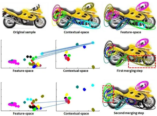
Representant computation: When the new C-BOVW dictionary is ob-tained, a set of represent for each final word is computed. In order to obtain a stratified number of represent related to the word densities, only one represent is assigned to the word with the minimum number of elements. Then, a pro-portional number of represent is computed for the rest of words by applying k-means and computing the mean vector for each of the word sub-clusters. With the final set of represent feature vectors, a normalized sentence of word occur-rences is computed for each sample in the training set, defining its probability density function of C-BOVW visual words. The whole C-BOVW procedure is formally described in Algorithm 1. An example of a two-iteration C-BOVW definition for a motorbike sample is shown in Figure 3. At the top of the figure, the initial spaces are shown. In the second row, the shared elements from the two spaces which maximize the percentage of matches for a given contextual word are shown. The contextual-space just considers thexand ycoordinates, and the 128 SIFT space is projected into a two-dimensional feature-space using the two principal components. Note that the feature descriptions for the two considered words are very close in the feature space though they belong to different visual words before merging. On the right of the figure the new merged feature cluster is shown within a dashed rectangle. The same procedure is applied for the second iteration of the merging procedure in the bottom row of the figure.
Sentence construction: After the definition of the new dictionary, a new test sample can be simply described using the Bag-Of-Visual-Words without the need of including geometrical information since it is implicitly considered in the new visual words. The sentence for the new sample is then computed by matching its descriptors to the visual words with the nearest represent. Finally, the test sentence can be learned and classified using any kind of classification strategy. In the next chapter, we explain the framework used to learn the CBOVW feature space.
Algorithm 1 Contextual Bag-Of-Visual-Words algorithm.
Require: D = {(x1, l1), ..,(xm, lm)}, where xi is an object sample of label li ∈ [1, .., n] for an-class problem,K clusters, and I merging steps.
Ensure: Representant R = {(r1, w1), ..,(rv, wb)}, where rv is a representant for wordwi,i∈[1, ..b] forb words. SentencesS ={(s1, l1), ..,(sm, lm)}, where si is the sentence of samplexi.
1: foreach sample xi ∈Ddo
2: Detect regions of interest for samplexi:
Xi = {(x1, y1, ρ11, ρ21, ρ31), ..,(xj, yj, ρ1j, ρ2j, ρ3j)}, where x and y are spatial co-ordinates normalized by the height and width of the image, and ρ1, ρ2, and ρ3 are ellipse parameters for affine region detectors.
3: Compute region descriptors: Xr
i ={r1, .., rj}, where rj is the description of thejth detected region of sample xi.
4: end for
5: Define a contextual-space C = {(c1, wC1), ..,(cq, wqC)} using k-means to define K contextual clusters, wherewC
i is theith word of the contextual-space. 6: Define a feature-space F = {(f1, wF1), ..,(fq, wFq)} using k-means to define K
feature clusters, wherewF
i is the ith word of the feature-space.
7: Initialize a contextual-feature relational matrixM:M(i, j) = 0, i, j∈[1, .., K] 8: InitializeW =∅ the list of feature words to be merged
9: forI merging steps do
10: updateM based on the contextual clusters and new feature clusters so that M(i, j) = d(C,F,i,j|wF )
j| , where d(C, F, i, j) returns the number of points from
contextual-space of word wC
i that belong to the feature-space jth wordwjF, and |wF
j |is the number of regions of the jth feature word.
11: Select the pair of positions with the maximum value for each row of M: maxj,kM(i, ),j6=k,∀i, where 0 0stands for all row positions.
12: W = W ∪(wF
j , wkF): Select the contextual word wCi and words wFj and wFk from the feature-space based on maxi(min(M(i, j), M(i, k))),∀j, k
13: end for
14: foreach pair (wF
j , wFk) in W do 15: updateF so thatwF
j ←wFk, and rename feature words so thatwFi , i∈[1, .., p] becomeswF
i , i∈[1, .., p−1] 16: end for
17: Compute representantR ={(r1, w1), ..,(rv, wb)}for the new F, where: zi = round
³
wi
min|wj|∀j
´
is the number of representant for word wi, computed using zi-means, and
{r1, .., rzi}representant are computed as the mean value for each sub-cluster of
wi, obtaining a stratified number of representant respect the words densities. 18: Compute sentencesS={(s1, l1), ..,(sm, lm)}for all training samples of all
3 Error-Correcting Output Codes
In this section, we review the Error-Correcting Output Codes framework, which is used to learn the previous C-BOVW sentences performing multi-class categorization as well as to rank the retrieval process that will be explained in the next section.
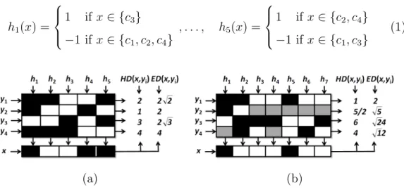
Given a set of N classes to be learnt in an ECOC framework, n different bi-partitions (groups of classes) are formed, andn binary problems (dichotomiz-ers) over the partitions are trained. As a result, a codeword of length n is obtained for each class, where each position (bit) of the code corresponds to a response of a given dichotomizer (coded by +1 or -1 according to their class set membership). Arranging the codewords as rows of a matrix, we define a coding matrix M, where M ∈ {−1,+1}N×n in the binary case. In fig. 4(a) we show an example of a binary coding matrix M. The matrix is coded us-ing 5 dichotomizers {h1, ..., h5} for a 4-class problem {c1, ..., c4} of respective codewords {y1, ..., y4}. The hypotheses are trained by considering the labeled training data samples{(ρ1, l(ρ1)), ...,(ρm, l(ρm))}for a set ofm data samples. The white regions of the coding matrix M are coded by +1 (considered as one class for its respective dichotomizer hj), and the dark regions are coded by -1 (considered as the other one). For example, the first classifier is trained to discriminate c3 against c1, c2, and c4; the second one classifies c2 and c3 againstc1 and c4, etc., as follows:
h1(x) = 1 if x∈ {c3} −1 if x∈ {c1, c2, c4} , . . . , h5(x) = 1 if x∈ {c2, c4} −1 if x∈ {c1, c3} (1) (a) (b)
Fig. 4. (a) Binary ECOC design for a 4-class problem. An input test codewordx is classified by class c2 using the Hamming or the Euclidean Decoding. (b) Example
of a ternary matrixM for a 4-class problem. A new test codewordxis classified by classc1 using the Hamming and the Euclidean Decoding.
During the decoding process, applying the n binary classifiers, a code x is obtained for each data sample ρin the test set. This code is compared to the
base codewords (yi, i∈[1, .., N]) of each class defined in the matrixM. And the data sample is assigned to the class with theclosest codeword. In fig. 4(a), the new codexis compared to the class codewords{y1, ..., y4}using the Hamming [41] and the Euclidean Decoding [42]. The test sample is classified by class c2 in both cases, correcting one bit error.
In the ternary symbol-based ECOC, the coding matrix becomesM ∈ {−1,0,+1}N×n. In this case, the symbol zero means that a particular class is not considered
for a given classifier. A ternary coding design is shown in fig. 4(b). The matrix is coded using 7 dichotomizers {h1, ..., h7} for a 4-class problem {c1, ..., c4} of respective codewords {y1, ..., y4}. The white regions are coded by 1 (consid-ered as one class by the respective dichotomizer hj), the dark regions by -1 (considered as the other class), and the gray regions correspond to the zero symbol (classes that are not considered by the respective dichotomizer hj). For example, the first classifier is trained to discriminate c3 againstc1 and c2 without taking into account classc4, the second one classifiesc2 againstc1,c3, and c4, etc. In this case, the Hamming and Euclidean Decoding classify the test data sample by class c1. Note that a test codeword can not contain the zero value since the output of each dichotomizer is hj ∈ {−1,+1}.
The analysis of the ECOC error evolution has demonstrated that ECOC cor-rects errors caused by the bias and the variance of the learning algorithm [43]1. The variance reduction is to be expected, since ensemble techniques address this problem successfully and ECOC is a form of voting procedure. On the other hand, the bias reduction must be interpreted as a property of the decoding step. It follows that if a pointρis misclassified by some of the learnt dichotomies, it can still be classified correctly after being decoded due to the correction ability of the ECOC algorithm. Non-local interaction between train-ing examples leads to different bias errors. Initially, the experiments in [43] show the bias and variance error reduction for algorithms withglobal behavior (when the errors made at the output bits are not correlated). After that, new analysis also shows that ECOC can improve performance of local classifiers (e.g., the k-nearest neighbor, which yields correlated predictions across the output bits) by extending the original algorithm or selecting different features for each bit [44].
1 The bias term describes the component of the error that results from systematic
errors of the learning algorithm. The variance term describes the component of the error that results from random variation and noise in the training samples and random behavior of the learning algorithm. For more details, see [43].
3.1 Coding designs
In this section, we review the state-of-the-art on coding designs. We divide the designs based on their membership to the binary or the ternary ECOC frameworks.
3.1.1 Binary coding
The standard binary coding designs are the one-versus-all [41] strategy and the dense random strategy [42]. In one-versus-all, each dichotomizer is trained to distinguish one class from the rest of classes. GivenN classes, this technique has a codeword length ofN bits. An example of an one-versus-all ECOC design for a 4-class problem is shown in fig. 5(a). The dense random strategy generates a high number of random coding matrices M of length n, where the values
{+1,−1}have a certain probability to appear (usually P(1) =P(−1) = 0.5). Studies on the performance of the dense random strategy suggested a length of n = 10 logN [42]. For the set of generated dense random matrices, the optimal one should maximize the Hamming Decoding measure between rows and columns (also considering the opposites), taking into account that each column of the matrix M must contain the two different symbols {−1,+1}. An example of a dense random ECOC design for a 4-class problem and five dichotomizers is shown in fig. 5(b). The complete coding approach was also proposed in [42]. Nevertheless, it requires the complete set of classifiers to be measured (2N−1−1), which usually is computationally unfeasible in practice.
(a) (b) (c)
(d) (e)
Fig. 5. Coding designs for a 4-class problem: (a) one-versus-all, (b) dense random, (c) one-versus-one, (d) sparse random, and (e) DECOC.
3.1.2 Ternary Coding
The standard ternary coding designs are the one-versus-one strategy [45] and the sparse random strategy [42]. The one-versus-one strategy considers all possible pairs of classes, thus, its codeword length is of N(N2−1). An example of an one-versus-one ECOC design for a 4-class problem is shown in fig. 5(c). The sparse random strategy is similar to the dense random design, but it includes the third symbol zero with another probability to appear, given by P(0) = 1−P(−1)−P(1). Studies suggested a sparse code length of 15 logN [42]. An example of a sparse ECOC design for a 4-class problem and five dichotomizers is shown in fig. 5(d). In the ternary case, the complete coding approach can also be defined.
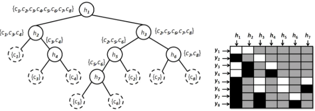
Due to the huge number of bits involved in the traditional coding strate-gies, new problem-dependent designs have been proposed [46][47][48]. The new techniques are based on exploiting the problem domain by selecting the representative binary problems that increase the generalization performance while keeping the code length small. The Discriminant ECOC (DECOC) of [48] is based on the embedding of discriminant tree structures derived from the problem domain. The binary trees are built by looking for the sub-sets of classes that maximizes the mutual information between the data and their respective class labels. As a result, the length of the codeword is only (n−1). The algorithm is summarized in table 1. In fig. 6, a binary tree structure for an 8-class problem is shown. Each node of the tree splits a sub-set of classes. Each internal node is embedded in the ECOC matrix as a column, where the white regions correspond to the classes on the left sub-sets of the tree, the black regions to the classes on the right sub-sets of the tree, and the gray re-gions correspond to the non-considered classes (set to zero). Another example of a DECOC design for a 4-class problem obtained by embedding a balanced tree is shown in fig. 5(e).2
Fig. 6. Example of a binary tree structure and its DECOC codification.
2 For further information about more recent coding designs the reader is referred
Table 1
DECOC algorithm.
DECOC: Create the Column Code Binary Tree as follows: Initialize LtoL0={{c1, .., cN}}
while |Lk|>0
1) Get Sk:Sk∈Lk, k∈[0, N −2]
2) Find the optimal binary partition BP(Sk) that maximizes the fast quadratic mutual information [48].
3) Assign to the column t of matrix M the code obtained by the new partition BP(Sk) ={C1, C2}.
4) Update the sub-sets of classesLk to be trained as follows: L0k =Lk\Sk
Lk+1 =L
0
k∪Ci iff |Ci|>1, i∈[1,2] 3.2 Decoding designs
In this section, we review the state-of-the-art on decoding designs. The de-coding strategies (independently of the rules they are based on) are divided depending if they were designed to deal with the binary or the ternary ECOC frameworks.
3.2.1 Binary decoding
The binary decoding designs most frequently applied are: Hamming Decoding [41], Inverse Hamming Decoding [51], and Euclidean Decoding [42].
• Hamming Decoding
The initial proposal to decode is the Hamming Decoding measure. This mea-sure is defined as follows:
HD(x, yi) = n X j=1 (1−sign(xjyj i))/2 (2)
This decoding strategy is based on the error correcting principles under the assumption that the learning task can be modeled as a communication prob-lem, in which class information is transmitted over a channel, and two possible symbols can be found at each position of the sequence [11].
• Inverse Hamming Decoding
The Inverse Hamming Decoding [51] is defined as follows: let ∆ be the matrix composed by the Hamming Decoding measures between the codewords of M. Each position of ∆ is defined by ∆(i1, i2) = HD(yi1, yi2). ∆ can be inverted to find the vector containing the N individual class likelihood functions by means of:
IHD(x, yi) = max(∆−1DT) (3)
where the values of ∆−1DT can be seen as the proportionality of each class codeword in the test codeword, and D is the vector of Hamming Decoding values of the test codeword x for each of the base codewords yi. The practi-cal behavior of the IHD showed to be very close to the behavior of the HD strategy [41].
• Euclidean Decoding
Another well-known decoding strategy is the Euclidean Decoding. This mea-sure is defined as follows:
ED(x, yi) = v u u tXn j=1 (xj−yj i)2 (4) 3.2.2 Ternary decoding
Concerning the ternary decoding, the state-of-the-art strategies are: Loss-based Decoding [42], and the Probabilistic Decoding [52].
• Loss-based Decoding
The Loss-based Decoding strategy [42] chooses the label `i that is most con-sistent with the predictions f (where f is a real-valued function f : ρ →R), in the sense that, if the data sampleρwas labeled`i, the total loss on example (ρ, `i) would be minimized over choices of `i ∈`, where ` is the complete set of labels. Formally, given a Loss-function model, the decoding measure is the total loss on a proposed data sample (ρ, `i):
LB(ρ, yi) = n
X
j=1
L(yijfj(ρ)) (5)
on the nature of the binary classifier. The two most common Loss-functions are L(θ) = −θ (Linear Loss-based Decoding (LLB)) and L(θ) = e−θ (Exponen-tial Loss-based Decoding (ELB)). The final decision is achieved by assigning a label to exampleρaccording to the classciwhich obtains the minimum score.
• Probabilistic Decoding
Recently, the authors of [52] proposed a probabilistic decoding strategy based on the continuous output of the classifier to deal with the ternary decoding. The decoding measure is given by:
P D(yi, F) = −log Y j∈[1,...,n]:M(i,j)6=0 P(xj =M(i, j)|fj) +K (6)
where K is a constant factor that collects the probability mass dispersed on the invalid codes, and the probability P(xj = M(i, j)|fj) is estimated by means of:
P(xj =yji|fj) = 1
1 +eyji(υjfj+ωj) (7)
where vectors υ and ω are obtained by solving an optimization problem [52]
• Loss-Weighted Decoding
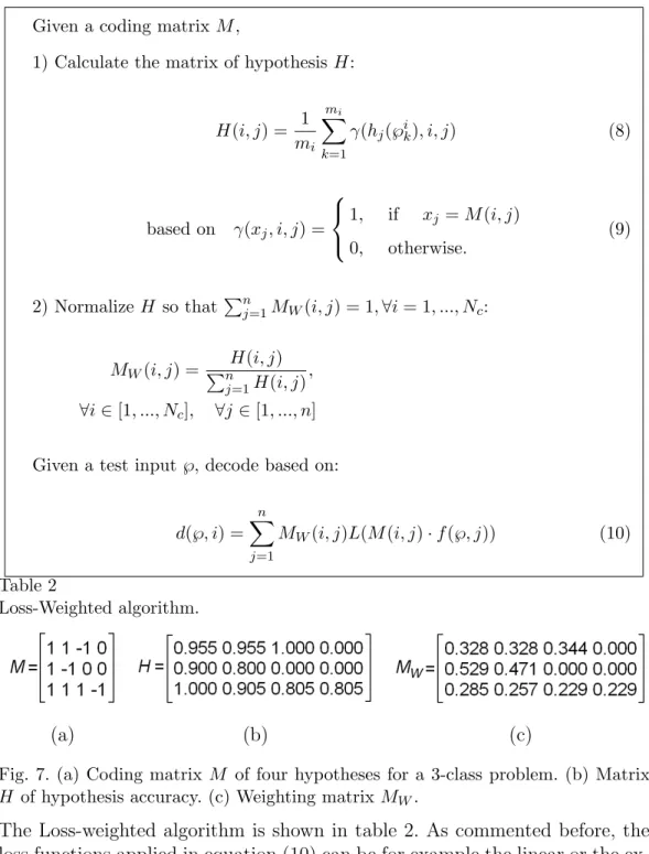
The main objective of the Loss-Weighted decoding is to find a weighting matrix MW that weights a loss function to adjust the decisions of the classifiers, either in the binary and in the ternary ECOC frameworks. To obtain the weighting matrix MW, we assign to each position (i, j) of the matrix of hypothesis H a continuous value that corresponds to the accuracy of the dichotomyhj classi-fying the samples of class i (8). We makeH to have zero probability at those positions corresponding to unconsidered classes (9), since these positions do not have representative information. The next step is to normalize each row of the matrix H so thatMW can be considered as a discrete probability density function (10). This step is very important since we assume that the probability of considering each class for the final classification is the same (independently of number of zero symbols) in the case of not having a priori information (P(c1) =...=P(cNc)). In fig. 7 a weighting matrix MW for a 3-class problem
with four hypothesis is estimated. Figure 7(a) shows the coding matrix M. The matrix H of fig. 7(b) represents the accuracy of the hypothesis classify-ing the instances of the trainclassify-ing set. The normalization of H results in the weighting matrix MW of fig. 7(c).3
3 Note that the presented Weighting Matrix M
W can also be applied over any decoding strategy.
Given a coding matrixM,
1) Calculate the matrix of hypothesisH:
H(i, j) = 1 mi mi X k=1 γ(hj(℘ik), i, j) (8) based on γ(xj, i, j) = 1, if xj =M(i, j) 0, otherwise. (9) 2) Normalize H so that Pnj=1MW(i, j) = 1,∀i= 1, ..., Nc: MW(i, j) = PnH(i, j) j=1H(i, j) , ∀i∈[1, ..., Nc], ∀j∈[1, ..., n] Given a test input℘, decode based on:
d(℘, i) = n X j=1 MW(i, j)L(M(i, j)·f(℘, j)) (10) Table 2 Loss-Weighted algorithm. (a) (b) (c)
Fig. 7. (a) Coding matrix M of four hypotheses for a 3-class problem. (b) Matrix H of hypothesis accuracy. (c) Weighting matrix MW.
The Loss-weighted algorithm is shown in table 2. As commented before, the loss functions applied in equation (10) can be for example the linear or the ex-ponential ones. The linear function is defined byL(θ) = θ, and the exponential loss function byL(θ) =e−θ, where in our caseθcorresponds toM(i, j)·fj(℘). Function fj(℘) may return either the binary label or the confidence value of applying the jth ECOC classifier to the sample℘.4
4 For further information about more recent decoding designs the reader is referred
4 ECOC-Rank
Retrieval systems retrieve huge amount of data for each query. Thus, sorting the results from most to less relevant cases is required. Based on the framework and application there exist different ways for ranking the results based on the associated criteria.
In the decoding process of the ECOC framework, a ”distance” associated to each class is computed. This ”distance” could be then interpreted as a ranking measure. But this ranking is the most trivial way for sorting the results. More-over, the output of the ECOC system does not take into account any semantic relationship among classes, which may be beneficial in retrieval applications. As an example of an image retrieval system, suppose the query of ”Dog”. In the feature space, it is possible that there exists high similarity between ”Dog” and ”Bike”, so based on features, the ranking will be higher for ”Bike” than for some other class which can be semantically more similar to ”Dog”, such as ”Cat”. On the other hand, it is easy to see that similarity based on features also is important, and thus, a tradeoff based on appearance and semantics is required. Thus, our goal is to embed class semantics and contextual informa-tion in the ranking process. For this purpose, we define two matrices that will be used to vote the ranking process: one based on adjacency and another one based on ontology. These matrices aren×n matrices forn number of classes, where each entry represents the similarity between two classes. By multiplying the ranking vector of the ECOC output by these matrices, we can improve the retrieval results. In the rest of this section we describe the design of the adjacency matrix, ontology matrix, and their use to modify the output ECOC ranking.
4.1 Adjacency Matrix MA
As we discussed, our goal is to enhance the primarily ranking based on ECOC output. First, we use class similarities in feature space and define an adjacency matrix.
There are different approaches in literature for measuring the similarity be-tween two classes, Support Vector Machines margins and the distance bebe-tween cluster centroid are two common approaches. Here, we follow a method similar to the second approach. However, just considering the cluster centroid would not be an accurate criteria for non-Gaussian data distributions. Instead, we re-cluster each class data into a few number of clusters and measure the mean distance of centroid of the new set of representant.
be converted to a measure of likelihood, which means that the more two classes are similar, the more the new measure among them should be higher. Thus, we compute the inverse of the distance for each element and normalize each column of the matrix to one to give the same relevance to each of the classes similarities. The details of this procedure are described in algorithm 3.
Table 3
Adjacency MatrixMA computation.
Given the class set c = {c1, c2, .., cn} and their associated data W = {Wc1, .., Wcn}forn classes
For each ci
1) Run k-means on Wci set and compute the cluster centroids for class ci asmi={mi1, .., mik}
Construct distance matrix MD as follows: For each pair of classes cp and cq
1)MD(p, q) =
Pk i=1
Pk
j=1δ(mpi,mqj)
k2 , beingδ a similarity function Convert distance matrix MD to adjacency matrixMA as follows: For each pair of classes cp and cq
1)MA(p, q) = MD1(p,q)
Normalize each column p of MA as follows: 1)MA(p, q) = PnMA(p,q)
i=1MA(i,p)
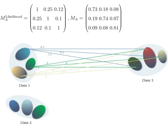
Look at the toy problem of Figure 8. In the example, for each class three representant are computed using k-means. Then the distance among all pairs of representant are computed for a pair of classes, obtaining an adjacency distance for that two classes as MD(1,3) = 8+10+9+7+9+8+79 .5+9.5+8.5 = 8.5. After that, the remaining positions of MD are obtained in the same way, obtaining the following distance matrix MD:
MD = 1 4 8.5 4 1 10 8.5 10 1
Finally, the adjacency matrix is computed changing the distance to a value of likelihood and normalizing each column of the matrix. Then we obtain the final adjacency matrix MA for the toy problem as:
MLikelihood A = 1 0.25 0.12 0.25 1 0.1 0.12 0.1 1 , MA= 0.73 0.18 0.08 0.19 0.74 0.07 0.09 0.08 0.81
Fig. 8. Toy problem for a 3-class classification problem. For each class, three repre-sentant are computed using k-means. Then the distance among all pairs of repre-sentant are computed for a pair of classes. This distance is used in next steps to fill the adjacency matrix MAvalues.
4.2 Ontology Matrix MO
The process up to here considered the relationship between classes by means of computational methods. However, some times no matter how good the system is, it needs the human knowledge. Here, we try to ”inject” human knowledge of semantic similarity between classes into the system.
Taxonomy based on ontology is a tree or hierarchical classification which is organized by subtype-supertype relationships or in another word parent-child relationship. For example, Dog is a subtype of Animal. The authors of Cal-tech256 data set compiled a taxonomy for all the categories included in their data set. Based on this taxonomy, we also defined a similar one for the MSR-CORID data set, which will be used to validate our methodology in the results section. Both taxonomies are shown in Figures 10 and 11, respectively.
Here we try to construct a similarity matrix like we did for the adjacency ma-trix, but now the similarity of classes is computed by means of the taxonomy tree.
Fig. 9. Example of the ontology distance computation of vertex v1 to the rest of
vertices. The steps of the distance computation are sorted and showed in red. The final ranking is shown in the last step of the distance computation. This final ranking is then normalized and used as a ontology likelihood.
In order to compute the distance among classes based on the taxonomy, we look for common ancestor of nodes within the tree. Each category is repre-sented as a leaf, and the non-leaf vertices correspond to abstract objects or super-categories. The less distance of the two leafs to their common ancestor, the less is their distance. We construct the similarity matrix by crawling the tree from a leaf and rank all other leaves based on their distance. When we start from each leaf and crawl up the tree, at each step the current node is being explored based on depth-first search algorithm. In this search, the less depth leaves get higher rank.
Finally, like in the case of the adjacency matrix, we need to convert distances into a measure of likelihood by inverting the values, and normalizing each col-umn of the ontology matrixMOto give the same importance for the taxonomy of all the classes. The whole process of computing the taxonomy distance and the ontology matrix is explained in algorithm 4 by means of recursive func-tions. Figure 9 shows an example of an ontology distance computation for the previous toy problem shown in Figure 8.
The final ontology matrix MO obtaining after computing all ranking from ontology distance and likelihood computation are the followings:
Table 4
Ontology MatrixMO computation.
Given the class set c={c1, c2, .., cn}and the taxonomy graph G For each leaf vertex vi in G, i ∈ [1, .., n], where n is the number of
classes
1) Visiting vertexvj =vi, Up Levell= 0, Depthd= 0 Position list for each vertexvp:MP(vp) = [Lvp, Dvp]
whereLvp is the level ofvp and Dvp is the depth of vp
2)Do while there are unvisited vertices 1)V isitV ertice(vj) Function VisitVertice(vp): Ifvp is not visited visitChild(vp) if∃ parent(vp) l=l+ 1 M(vp) = [l, d]
V isitV ertice(parent(vp)) Function VisitChild(vp): for each childvc
p ofvp: ifvc
p has not been visited: if child(vc p) ! =∅ VisitChild(vp) else d=d+ 1 M(vp) = [l, d] 3) Filling the ranks
r= 0 forν = [1, ..,max(l)] for ω= [1, ..,max(d)] if vq|MP(vq) = [ν, ω] is a leaf vertex ofG MO(i, q) =r r=r+ 1
Convert distance matrix MD to ontology matrixMO as follows: For each pair of classes cp and cq
1)MO(p, q) = MO1(p,q)
Normalize each column p of MO as follows: 1)MO(p, q) = PnMO(p,q) i=1MO(i,p) MORanking= 1 2 3 4 5 6 2 1 3 4 5 6 4 3 1 2 5 6 4 3 2 1 5 6 5 2 3 4 1 6 , MLikelihood O = 1.0000 0.5000 0.3333 0.2500 0.2000 0.1667 0.5000 1.0000 0.3333 0.2500 0.2000 0.1667 0.2500 0.3333 1.0000 0.5000 0.2000 0.1667 0.2500 0.3333 0.5000 1.0000 0.2000 0.1667 0.2000 0.5000 0.3333 0.2500 1.0000 0.1667
MO= 0.4082 0.2041 0.1361 0.1020 0.0816 0.0680 0.2041 0.4082 0.1361 0.1020 0.0816 0.0680 0.1020 0.1361 0.4082 0.2041 0.0816 0.0680 0.1020 0.1361 0.2041 0.4082 0.0816 0.0680 0.0816 0.2041 0.1361 0.1020 0.4082 0.0680 0.0680 0.1361 0.1020 0.0816 0.2041 0.4082
4.3 Altering ECOC output rank using MA and MO
Given the output vectorD={d1, .., dn} of the ECOC design, wheredi repre-sents the distance of a test sample to codeword i of the coding matrix, first, we convert the vector Dto a measure of likelihood by inverting each position of D and normalizing the vector as follows:
DL= P 1 n i=1d1i ½ 1 d1 , .., 1 dn ¾ (11)
Then, using the previous MA and MO matrices, the new altered rank R is obtained by means of a simple multiplication, as shown in eq.(12).
Fig. 10. A taxonomy of Caltech 256 categories created by hand. At the top level these are divided into animate and inanimate objects. Green categories contain images that were borrowed from Caltech 101. A category is colores red if it overlaps with some other category (such as ’dog’ and ’greyhound’).
5 Results
We divide the results into two types, validating the C-BOVW methodology and validating the ECOC-Rank methodology.
5.1 Contextual Bag-Of-Visual Words
Before the presentation of the results of the C-BOVW methodology, first, we discuss the data, methods, software details, and validation protocol of the experiments.
Data: The data used in the experiments consist of 15 categories from public Caltech 101 [54] and Caltech 256 [55] repository data sets. One sample for each category is shown in Figure 12. For each category, 50 samples were used, 10 samples to define the BOW and another 40 images to define new test sentences.
Fig. 12. Considered categories from the Caltech 101 and Caltech 256 repositories. Methods: We compare the C-BOVW with the classical BOVW model. For both methods, the same initial set of regions is considered in order to compare both strategies at the same conditions. About 200±20 object regions are found by image using the Harris-Affine detector [56] and described using the SIFT descriptor [3]. The visual words are obtained using the public open source k-means software from [57]. After computing the final words and representant, multi-class classification is performed using an one-versus-one ECOC method-ology with different base classifiers: Mean Nearest Neighbor (NMC), Fisher Discriminant Analysis with a previous 99% of PCA (FLDA), Gentle Adaboost with 50 iterations of decision stumps (G-ADA), Linear Support Vector Ma-chines with the regularization parameter C = 1 (Linear SVM), and Support Vector Machines with RBF Kernel with C and γ parameters set to 1 (RBF SVM)5. Finally, we use the Linear Loss-weighted decoding to obtain the class label [58].
5 We decided to keep the parameter fixed for the sake of simplicity and easiness of replication of the experiments, though we are aware that this parameter might not be optimal for all data sets.
Software details: The project was implemented in Python and the data were stored in MySQL data set. For the multi-class classification we used the Error-Correcting Output Codes library implemented in Matlab/Octave 6.
Validation protocol: We used the sentences obtained by the 50 samples of each category and performed stratified ten-fold cross-validation evaluation.
5.1.1 Caltech 101 and 256 classification
In this experiment, we started classifying from three Caltech categories in-creasing by 2 up to 15. For each step, different number of visual words are com-puted: 30, 40, and 50. These numbers are obtained by performing ten iterations of the merging procedure (experimentally tested). In order to compare the BOVW and C-BOVW methods at the same conditions, the same detected re-gions and descriptions are used for all the experiments. The order in which the categories are considered is the following: (1-3) airplane, motor-bike, watch, (4-5) tripod, face, (6-7) ketch, diamond-ring, (8-9) teddy-bear, t-shirt, (10-11) desk-globe, backpack, (12-13) hourglass, teapot, (14-15) cowboy-hat, and umbrella. The obtained results applying ten-fold cross-validation are graphi-cally shown in Figure 13 for the different ECOC base classifiers. Note that the classification error significantly varies depending on the ECOC classifier. In particular, Gentle Adaboost obtains the best results, with a classification error inferior to 0.2 in all the tests when using 30 C-BOVW words. Independently of the ECOC classifier, in most of the experiments the C-BOVW model obtains errors inferiors to those obtained by the classical BOVW. BOVW only obtains slightly better results in the case of Gentle Adaboost for eleven classes and 50 visual words.
An important remark of the C-BOVW model is about the selection of the number of merging iterations. This parameter has a decisive impact over the generalization capability of the new visual dictionary. First iterations of the merging procedure use to fuse very close feature-words which belong to differ-ent visual words whereas final merging iterations fuse more far regions of the feature-space. Thus, a large number of iterations could be detrimental since the new merged words could be too general for discriminating among sentences of different object categories. Thus, this parameter should be estimated for each particular problem domain (i.e. applying cross-validation over a training and a validation subset). In the previous experiment we checked that ten merging iterations obtains significant performance improvements, though we are aware that this parameter could be not optimal for all the data sets.
NMC FLDA
G-ADA Linear SVM
RBF SVM
Fig. 13. Classification results for the Caltech categories using BOVW and C-BOVW dictionaries for different number of visual words and ECOC base classifiers.
5.2 Ranking ECOC output
Before the presentation of the results of the ECOC-Rank methodology, first, we discuss the data, methods and parameters, software details, and validation protocol of the experiments.
Data:The data used in our experiments consist on two public data sets: Cal-tech 256 [55] and ’Microsoft Research Cambridge Object Recognition Image data set’ (MRCORID) [59].
Methods and parameters: We use the same methods and parameters for computing BOVW and CBOVW than at the previous experiments for the Cal-tech 256 [55] data set and ’Microsoft Research Cambridge Object Recognition Image data set data set’ [59]. For the ECOC classification, One-versus-one method with Gentle Adaboost with 50 decision stumps and RBF SVM clas-sifiers has been used. We use the Linear Loss-weighted decoding to obtain the class label [58]. For the adjacency matrix construction, the k parameter of k-means has been experimentally set to 3. For ranking the hist count we looked for one to seven matches at the first 15 positions using vector ontology and semantic distances of 0.001 and 0.0001.
Software details:The project was implemented in Python and the data was stored in MySQL data set. Error-Correcting Output Codes and Ranking code were implemented in Matlab.
Validation measurements: In order to analyze the retrieval efficiency, we defined an ontology distance based on taxonomy trees to look for the retrieved classes at the first positions of the ranking process based on the confusion matrix.
As explained in the previous section, the ranking result R is a sorted set of classes, where the first items have the highest rank.
In retrieval problems, we are looking for an interval of positions to look for the target objects. In our case, retrieving classes, we need to define a validation measure among classes. For this purpose, we define an ontology distance m based on the taxonomy tree and adjacency matrices. Each class ci in R is accepted if its ontology distancedi compared to the true label class is less than m. The accepted results at the end of the list R are not desired, so another parameter k (positions) is used to analyze the results of the first positions of the ranking. If there are more than N (accepted count) accepted classes based on the value of m at the first positions defined by k, then we achieve a test hit. In order to perform a realistic analysis, we included this validation procedure in a stratified 10-fold evaluation procedure. The algorithm that summarizes the retrieval validation is shown in table 5.
Table 5
ECOC-Rank evaluation.
Given the sorted list of classes based on their rank R={r1, .., rn} For each item ri in the top k positions of R
acceptedCount= 0
1)d=OntologyDistance(ri, T rueLabel) 2) ifd < mthen acceptedCount+ = 1 1) If acceptedCount > N thenHit
We also apply statistical Friedman and Nemenyi test to look for statistical significance among the obtained performances [60].
5.2.1 Caltech 256 retrieval evaluation
Some samples of the Caltech 256 data set are shown in Figure 14. The ontology matrix MO computed for this data set and BOVW features are shown in Figure 15. In this case, we defined an ontology distance of 0.001 and 0.0001 for Adaboost ECOC base classifier based on the ontology tree of Figure 10 and the ontology distance defined in previous chapters. For both distances we computed the CBOVW and BOVW features for this data set for different values of thek first positions and number of hits. The results are shown in the performance surfaces of Figure 16 and 17, respectively. The performances are also shown in Table 6 estimated as the mean performance surface for each experiment. We have used this performance evaluation since it is more general than the classical ROC curve.
Fig. 14. Caltech 256 samples. Table 6
Performances of Caltech 256 data set for different methods and parameters using Gentle Adaboost ECOC base classifier and ontology distance evaluation.
Problem Adjacency Ontology Adjacency & Ontology ECOC-raw m=0.001 CBOVW 0.4635 0.6902 0.4974 0.5604
m=0.001 BOVW 0.4394 0.6901 0.4389 0.5530 m=0.0001 CBOVW 0.0843 0.1485 0.0829 0.0809 m=0.0001 BOVW 0.0718 0.1479 0.0719 0.0785
Comparing CBOVW and BOVW methods for all the previous experiments and both classifiers, we compute the mean rank for both strategies. The rank-ings are obtained estimating each particular ranking rji for each problem i and each method j, and computing the mean ranking R for each method as Rj = 1
N
P
irji, whereN is the total number of problems. We obtained a rank-ing for CBOVW of 1.00 and a rankrank-ing for BOVW of 2.00. This means that though the improvement of CBOVW is of small difference in most of the ex-periments, it achieves always the best performance, and CBOVW is preferred as the first choice for this particular data set using Adaboost base classifier.
Fig. 15. Ontology matrixMO computed for the Caltech data set and CBOVW. Now we compare if any of the four variants of ranking strategies is preferred against the rest. For this purpose, considering all previous experiment, we compute the mean rank of each strategy as explained before. The obtained ranks are shown in Table 7.
Table 7
Ranking of Caltech 256 data set for the different ECOC-Rank configurations con-sidering all experiments with ontology distance evaluation.
Adjacency Ontology Adjacency & Ontology ECOC-raw 3.2500 1.0000 3.3750 2.5000
In order to analyze if the difference between methods ranks are statistically significant, we apply the Friedman and Nemenyi tests. In order to reject the null hypothesis that the measured ranks differ from the mean rank, and that the ranks are affected by randomness in the results, we use the Friedman test. The Friedman statistic value is computed as follows:
X2 F = 12N k(k+ 1) X j R2 j − k(k+ 1)2 4 (13)
In our case, with k = 4 ranking designs to compare and N = 4 experiments, X2
Original ECOC vs Adjacency
Original ECOC vs Ontology
Original ECOC vs Adjacency and Ontology
Fig. 16. Results on Caltech 256 data set for ontology distancem=0.0001 and Gentle Adaboost ECOC base classifier. Left column using BOVW and right column using CBOVW.
Iman and Davenport proposed a corrected statistic:
FF = (N −1)X2 F N(k−1)−X2 F (14)
Original ECOC vs Adjacency
Original ECOC vs Ontology
Original ECOC vs Adjacency and Ontology
Fig. 17. Results on Caltech 256 data set for ontology distancem=0.001 and Gentle Adaboost ECOC base classifier. Left column using BOVW and right column using CBOVW.
experiments, FF is distributed according to the F distribution with ((k − 1),(k −1)(N − 1)) degrees of freedom (3 and 9 in our case). The critical value ofF(3,9) for 0.05 is 3.86. As the value of FF is higher than 3.86 we can reject the null hypothesis. One we have checked for the non-randomness of the results, we can perform a post hoc test to check if one of the techniques can be singled out. For this purpose we use the Nemenyi test - two techniques are