Novel Object-Based Filter for Improving Land-Cover Classification of Aerial Imagery with Very High Spatial Resolution

(1)

remote sensing

Article

Novel Object-Based Filter for Improving Land-Cover

Classification of Aerial Imagery with Very High

Spatial Resolution

Zhiyong Lv1, Wenzhong Shi2,*, Jón Atli Benediktsson3and Xiaojuan Ning1

1 _{School of Computer Science and Engineering, Xi’An University of Technology, Xi’an 710048, China;}

[email protected] (Z.L.); [email protected] (X.N.)

2 _{Department of Land Surveying and Geo-Informatics, the Hong Kong Polytechnic University, Hong Hom,}

Hong Kong 999000, China

3 _{Faculty of Electrical and Computer Engineering, University of Iceland, Reykjavik IS 107, Iceland;}

[email protected]

* Correspondence: [email protected]; Tel.: +86-159-8986-8038

Academic Editors: Yuei-An Liou, Chyi-Tyi Lee, Yuriy Kuleshov, Jean-Pierre Barriot, Chung-Ru Ho, Jose Moreno, Richard Gloaguen and Prasad S. Thenkabail

Received: 4 October 2016; Accepted: 9 December 2016; Published: 15 December 2016

Abstract:Land cover classification using very high spatial resolution (VHSR) imaging plays a very important role in remote sensing applications. However, image noise usually reduces the classification accuracy of VHSR images. Image spatial filters have been recently adopted to improve VHSR image land cover classification. In this study, a new object-based image filter using topology and feature constraints is proposed, where an object is considered as a central object and has irregular shapes and various numbers of neighbors depending on the nature of the surroundings. First, multi-scale segmentation is used to generate a homogeneous image object and extract the corresponding vectors. Then, topology and feature constraints are proposed to select the adjacent objects, which present similar materials to the central object. Third, the feature of the central object is smoothed by the average of the selected objects’ feature. This proposed approach is validated on three VHSR images, ranging from a fixed-wing aerial image to UAV images. The performance of the proposed approach is compared to a standard object-based approach (OO), object correlative index (OCI) spatial feature based method, a recursive filter (RF), and a rolling guided filter (RGF), and has shown a 6%–18% improvement in overall accuracy.

Keywords:image filter; very high spatial resolution (VHSR) aerial image; multi-scale segmentation; land cover classification

1. Introduction

Very high spatial resolution (VHSR) remote sensing imagery, such as aerial images and unmanned aerial vehicle (UAV) images, reveal ground details, including texture, geometry, and topology, and thus provide an outstanding visual performance [1]. Therefore, classification of VHSR images for various applications has received much research interest [2–4]. However, compared with the classification of high spatial resolution hyperspectral remote sensing images , the classification of remote sensing images with a high spatial resolution but a relatively low spectral resolution (such as images obtained by airborne or UAV) has become challenging. Given the improvement in spatial resolution, several zones may appear too small and heterogeneous when a VHSR image is processed by multi-scale segmentation. These zones may be meaningless relative to the classes of interest. Furthermore, the increase in spatial resolution enhances the correlative strength of the pixels of the intra-class. Consequently, the spectral signatures inside a target become highly heterogeneous, and different Remote Sens.2016,8, 1023; doi:10.3390/rs8121023 www.mdpi.com/journal/remotesensing

(2)

Remote Sens.2016,8, 1023 2 of 14

targets present increasingly similar spectra. A high intra-class and a low inter-class variability reduce the separability of different land cover classes in the spectral domain [1,5,6].

Numerous strategies have been adopted to overcome these challenges in VHSR image classification. Spatial–spectral feature extraction is the most popular approach. It aims to complement the insufficiency of spectral information by exploiting the spatial features of a ground object [7,8]. These features, such as the pixel shape index (PSI) [9], the pixel spatial feature set [10], and structural features, are exploited through mathematical morphology and its related models [11–15]. In addition, object-based image analysis is also a new paradigm for VHSR image classification [16]. The object-based approach usually begins with segmentation to generate an image object, which is a group of pixels that are spectrally similar and spatially contiguous. The application of the object-based approach in practical situations has been studied extensively [13,17–20]. The object-based approach has several advantages over pixel-based VHSR image classification in terms of classification accuracy [21,22].

Image filters, especially the edge-preserving filter, have recently been proposed to smooth noise in images with a high spatial resolution and improve land cover classification accuracy. Edge-preserving filters have been adopted in many applications [23–25]. For example, Kang et al., proposed a spectral–spatial classification framework based on an edge-preserving filter and obtained a significantly improved classification accuracy [26]. They also presented a recursive filter combined with image fusion to enhance image classification [27]. Xia et al., proposed a method that combines subspace independent component analysis and a rolling guidance filter for the classification of hyperspectral images with high spatial resolution [28]. Experimental results showed that the proposed method gives a better accuracy than the traditional approach without the use of image filtering. From the application viewpoint, these simple yet effective approaches imply the many potential applications of VHSR images.

In this study, we adopted the idea of image filters and extended it to the context of the object-based approach. We refer to this adoption–extension approach as “object filter based on topology and features” (OFTF). We used the unique capabilities of the object-based image technique, which allows the noise in a VHSR image to be addressed in a multi-scale object manner. To achieve this purpose, first, a popular multi-scale algorithm-Fractal Net Evolution Algorithm (FNEA) which was embedded in the eCognition software was adopted to generate image objects [29,30]. FNEA, which is a widely used multi-scale segmentation algorithm, was first introduced by Batz and Schape. This algorithm quickly became one of the most important segmentation algorithms within the object-based analysis domain [30]. The basic idea of the algorithm is a bottom-up region merging technique. It starts with each image pixel as a separate object. Subsequently, pairs of image objects are merged into larger objects. The process terminates when no pair of objects satisfies the merging criterion. Second, the segmented object was exported as a vector with corresponding spectral features, such as the mean or the standard deviation of the pixels within an object for a band. In this case, a target usually exists as a group of objects that are similar in features and spatially continuous to allow for the smoothing of the difference among the objects from one target. To demonstrate the effectiveness of the proposed OFTF approach, we compared it with the original object-based approach (OO) and OCI [19] through image classification. In addition, two relatively new approaches, the recursive filter (RF) [27] and the rolling guided filter (RGF) [28], which have been applied successfully to high-resolution image classification, were compared with the proposed OFTF approach.

The remainder of this paper is organized as follows. Section 2 details the proposed OFTF approach. Section3presents the experimental setup and the results. Section4gives the discussion on the experimental results. Section5provides the conclusion.

2. Proposed Object Filter Based on Topology and Feature Constraints

The aim of the proposed OFTF is to improve the classification of VHSR images by smoothing the noise of the ground target in an object manner. Due to the complexity and uncertainty of the spatial arrangement of segmented objects, the proposed OFTF is based on a simple assumption: the objects

(3)

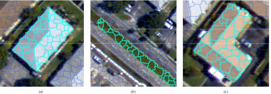
comprising a target usually have strong correlations with one another and present spatial continuity. As shown in Figure1, regardless of the shape of the target (e.g., rectangle, line, or “L”), its units are subject to the abovementioned assumption.

Remote Sens. 2016, 8, 1023 3 of 14

continuity. As shown in Figure 1, regardless of the shape of the target (e.g., rectangle, line, or “L”), its units are subject to the abovementioned assumption.

Figure 1. Performance example of a target’s objects in a remote sensing image scene, (a) “Rectangle”-building; (b) “Line-shape”-meadow; and (c) “L”-building.

In this case, several pre-processing steps, such as multi-scale segmentation and exporting the corresponding object’s vector, are necessary when the proposed OFTF approach is used. As shown in Figure 2, the proposed approach consists of the following three consecutive main steps (labeled as a dotted line).

1. Topology constraint: Based on the object’s vector, the neighboring object that touches the central object in the topology is obtained.

2. Feature constraint: In the feature space, the object in the set of the touched neighboring object that is dissimilar to the central object should be excluded. Details of how to judge the “dissimilarity” are presented in Section 2.2.

3. The feature of the central object is smoothed through the corresponding feature of the remaining neighboring objects. Each step is discussed in detail below.

Y Y ① ③ ② ④ ⑤ ⑥ ① ③ ② ④ ⑤ ⑥ (a) (b) [ ( ) ( ), ( ) ( )] sur a a a a O ∈m O R O m O R O− ×δ + ×δ

Figure 2. Flowchart of the proposed approach.

In this case, several pre-processing steps, such as multi-scale segmentation and exporting the corresponding object’s vector, are necessary when the proposed OFTF approach is used. As shown in Figure2, the proposed approach consists of the following three consecutive main steps (labeled as a dotted line).

2. Feature constraint: In the feature space, the object in the set of the touched neighboring object that is dissimilar to the central object should be excluded. Details of how to judge the “dissimilarity” are presented in Section2.2.

Remote Sens. 2016, 8, 1023 3 of 14

continuity. As shown in Figure 1, regardless of the shape of the target (e.g., rectangle, line, or “L”), its units are subject to the abovementioned assumption.

In this case, several pre-processing steps, such as multi-scale segmentation and exporting the corresponding object’s vector, are necessary when the proposed OFTF approach is used. As shown in Figure 2, the proposed approach consists of the following three consecutive main steps (labeled as a dotted line).

2. Feature constraint: In the feature space, the object in the set of the touched neighboring object that is dissimilar to the central object should be excluded. Details of how to judge the “dissimilarity” are presented in Section 2.2.

Y Y ① ③ ② ④ ⑤ ⑥ ① ③ ② ④ ⑤ ⑥ (a) (b) [ ( ) ( ), ( ) ( )] sur a a a a O ∈m O R O m O R O− ×δ + ×δ

Figure 2. Flowchart of the proposed approach. Figure 2.Flowchart of the proposed approach.

(4)

Remote Sens.2016,8, 1023 4 of 14

2.1. Topology Constraint

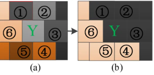
Compared with spectral features, topology may include information on geographic location, spatial arrangement, and geometry. This information is usually studied in the spatial analysis of geographic information systems (GIS). In addition, topology can be described in the VHSR remote sensing imagery. When an image was segmented into multi-scale image objects, a target consists of a group of objects which are spatially continuous. In this study, topology was introduced to reveal the spatial relationship between the central object and its neighboring objects. A topology called “TOUCH” was used as the spatial constraint for the proposed object filter. “TOUCH” represents the condition in which the central object and an adjacent object share a common boundary (or a part of a common boundary) with no gaps and overlaps. A group of objects that consists of a given target are usually spatially continuous. Therefore, this topology constraint can be regarded as spatial knowledge for image analysis.

As shown in Figure3, each block symbolizes an image object, and similar colors indicate the difference of the same material for a target. “Y” is a central object. Therefore, objects 1–6 touch “Y” according to our proposed topology constraint.

Remote Sens. 2016, 8, 1023 4 of 14

2.1. Topology Constraint

Compared with spectral features, topology may include information on geographic location, spatial arrangement, and geometry. This information is usually studied in the spatial analysis of geographic information systems (GIS). In addition, topology can be described in the VHSR remote sensing imagery. When an image was segmented into multi-scale image objects, a target consists of a group of objects which are spatially continuous. In this study, topology was introduced to reveal the spatial relationship between the central object and its neighboring objects. A topology called “TOUCH” was used as the spatial constraint for the proposed object filter. “TOUCH” represents the condition in which the central object and an adjacent object share a common boundary (or a part of a common boundary) with no gaps and overlaps. A group of objects that consists of a given target are usually spatially continuous. Therefore, this topology constraint can be regarded as spatial knowledge for image analysis.

As shown in Figure 3, each block symbolizes an image object, and similar colors indicate the difference of the same material for a target. “Y” is a central object. Therefore, objects 1–6 touch “Y” according to our proposed topology constraint.

Figure 3. Example of an object filter based on topology and feature constraints. (a) 1–6 are neighboring objects around central object Y. (b) Filtered result.

2.2. Feature Constraint

When the central object “Y” is located at the interior of a target, the adjacent surrounding objects are the same material of the target. However, when the central object “Y” is located at the boundary between different targets with a different material, smoothing the feature of “Y” by using all topology-touched objects is unreasonable. Therefore, the feature constraint is introduced to exclude objects that are different from the material of the central object.

To achieve this purpose, the difference among the objects that have the same material as the central object are denoted by the standard deviation and mean value of the pixels in the central object. Therefore, in the case of the topology constraint, the feature is introduced as another constraint in the spectral domain, the feature constraint is provided as Equation (1).

{

|

[ (

)

(

), (

)

(

)]}

b b b b b b b sur i i c c c c

O

=

O

∈

m O

− ×

R

δ

O

m O

+ ×

R

δ

O

(1) where b sur

O is the set of objects that satisfies the topology and feature constraints surrounding the

central object “c”, “b” is the b-th spectral band. m O( cb)_andδ(Ocb)_{are the mean and the standard}

deviation of band “b” of the central object, respectively. R is the relaxation parameter to ensure that

the constraint has general adaptability. It controls the degree of constraint in the feature domain.

When R = 0, the feature constraint is “ b ( b)

i c

O = m O ,” and a large R implies a large relaxation range

of the feature constraint. A suitable R is the key to obtaining a reasonable filtered result. If R is

excessively small, the relaxation would be too strict to cover the “variety” of different objects that

belong to the same target. If R is excessively large, more noise will be smoothed, but the object having

a material that is different from that of the central object will be introduced to smooth the central object’s feature.

Figure 3.Example of an object filter based on topology and feature constraints. (a) 1–6 are neighboring objects around central object Y. (b) Filtered result.

2.2. Feature Constraint

When the central object “Y” is located at the interior of a target, the adjacent surrounding objects are the same material of the target. However, when the central object “Y” is located at the boundary between different targets with a different material, smoothing the feature of “Y” by using all topology-touched objects is unreasonable. Therefore, the feature constraint is introduced to exclude objects that are different from the material of the central object.

To achieve this purpose, the difference among the objects that have the same material as the central object are denoted by the standard deviation and mean value of the pixels in the central object. Therefore, in the case of the topology constraint, the feature is introduced as another constraint in the spectral domain, the feature constraint is provided as Equation (1).

Osurb = n Ob_i O b i ∈[m(Obc)−R×δ(Ocb),m(Obc) +R×δ(Ocb)] o (1) whereOb

sur is the set of objects that satisfies the topology and feature constraints surrounding the central object “c”, “b” is theb-thspectral band. m(Obc) andδ(Obc)are the mean and the standard deviation of band “b” of the central object, respectively.Ris the relaxation parameter to ensure that the constraint has general adaptability. It controls the degree of constraint in the feature domain. When R= 0, the feature constraint is “Ob

i =m(Obc),” and a largeRimplies a large relaxation range of the feature constraint. A suitableRis the key to obtaining a reasonable filtered result. IfRis excessively small, the relaxation would be too strict to cover the “variety” of different objects that belong to the same target. IfRis excessively large, more noise will be smoothed, but the object having a material that is different from that of the central object will be introduced to smooth the central object’s feature.

(5)

Remote Sens.2016,8, 1023 5 of 14

In the proposed OFTF approach, the relationship among the feature constraints of each band is denoted by “AND”. In other words, a neighboring object can only be applied to smooth the feature of a central object until the feature constraints of each band for an object satisfy Equation (1).

2.3. Smoothing the Feature of the Central Object

In the case of topology and feature constraints, object setObcis obtained. The elements of this set meet the spatial and feature constraints. The proposed OFTF approach smooths the central object through the average ofOcb, i.e., by:

OFTF(Ob_c) = 1 N N

∑

i=1 Ob_i (2)

whereNis the total number of objects that satisfy the topology and feature constraints surrounding the central object. Therefore, the filtered feature of each band for the central object can be calculated with Equation (2).

It is worth noting that it is difficult to utilize the topology information for an image object directly. Therefore, from the technical point of view, a series of transformation is adopted. The workflow of OFTF is presented: First, the spectral feature and the topology information can be transformed into a shapefile with the aid of eCognition software. (The shapefile format is a popular geospatial vector data format for geographic information system). Then, a customize application was developed based on ArcEngine 10.0 for realizing the proposed OFTF. Finally, the filtered value of each image object can be exported, and the format can be customized for classification. To promise the repeatability of the proposed approach, the sourcing code of the customize application can be obtained from the first author.

3. Experimental Section

Three VHSR images acquired by an airborne platform were utilized to validate the feasibility and effectiveness of the proposed OFTF approach through classification. Three parts were designed to achieve the objectives. First, the images were described for each experiment. Second, an experiment was performed to investigate the adaptability and parameter sensitivity of the proposed approach for classification. Finally, the proposed OFTF was compared with the original object-based approach and two state-of-the-art approaches [27,28].

3.1. Data Sets

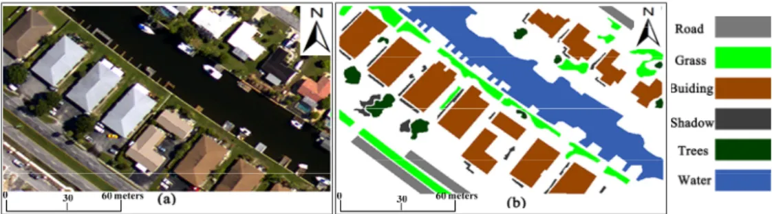
As shown in Figure4a, the first image was acquired with an airborne ADS80 sensor. The relative flying height was approximately 3000 m, and the spatial resolution was 0.32 m. The size of the image is 560×360 pixels. The aerial image was used to analyze the sensitivity of the parameters of the proposed OFTF for classification. Six interesting classes of this image were classified. These six classes were water, shadow, grass, trees, road, and building. The ground reference is shown in Figure4b.

In the proposed OFTF approach, the relationship among the feature constraints of each band is denoted by “AND”. In other words, a neighboring object can only be applied to smooth the feature of a central object until the feature constraints of each band for an object satisfy Equation (1).

2.3. Smoothing the Feature of the Central Object

In the case of topology and feature constraints, object set

b c

O

is obtained. The elements of this set meet the spatial and feature constraints. The proposed OFTF approach smooths the central object through the average of

b c O , i.e., by: 1

1 (

b

)

N b c i i

OFTF O

O

N

=



(2)

where

N

is the total number of objects that satisfy the topology and feature constraints surrounding

the central object. Therefore, the filtered feature of each band for the central object can be calculated with Equation (2).

It is worth noting that it is difficult to utilize the topology information for an image object directly. Therefore, from the technical point of view, a series of transformation is adopted. The workflow of OFTF is presented: First, the spectral feature and the topology information can be transformed into a shapefile with the aid of eCognition software. (The shapefile format is a popular geospatial vector data format for geographic information system). Then, a customize application was developed based on ArcEngine 10.0 for realizing the proposed OFTF. Finally, the filtered value of each image object can be exported, and the format can be customized for classification. To promise the repeatability of the proposed approach, the sourcing code of the customize application can be obtained from the first author.

3. Experimental Section

Three VHSR images acquired by an airborne platform were utilized to validate the feasibility and effectiveness of the proposed OFTF approach through classification. Three parts were designed to achieve the objectives. First, the images were described for each experiment. Second, an experiment was performed to investigate the adaptability and parameter sensitivity of the proposed approach for classification. Finally, the proposed OFTF was compared with the original object-based approach and two state-of-the-art approaches [27,28].

3.1. Data Sets

As shown in Figure 4a, the first image was acquired with an airborne ADS80 sensor. The relative flying height was approximately 3000 m, and the spatial resolution was 0.32 m. The size of the image is 560 × 360 pixels. The aerial image was used to analyze the sensitivity of the parameters of the proposed OFTF for classification. Six interesting classes of this image were classified. These six classes were water, shadow, grass, trees, road, and building. The ground reference is shown in Figure 4b.

Figure 4. First study area: (a) Aerial image with 0.32 m spatial resolution and (b) Ground reference data.

(6)

Remote Sens.2016,8, 1023 6 of 14

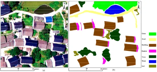
The second image was acquired with a Canon-5D-Mark2 camera mounted on an unmanned aerial vehicle (UAV) platform. The area is located in YingTan City, Jiang Xi Province, southern China. This VHSR image was used to test the feasibility and effectiveness of the proposed approach for classification. The image has a size of 1400×1000 pixels and 0.1 m spatial resolution, as shown in Figure5a. This image presents a typical country area in China and includes seven classes, namely, grass, road, building, shadow, trees, water, and soil. The ground reference is shown in Figure5b.

Remote Sens. 2016, 8, 1023 6 of 14

The second image was acquired with a Canon-5D-Mark2 camera mounted on an unmanned aerial vehicle (UAV) platform. The area is located in YingTan City, Jiang Xi Province, southern China. This VHSR image was used to test the feasibility and effectiveness of the proposed approach for classification. The image has a size of 1400 × 1000 pixels and 0.1 m spatial resolution, as shown in Figure 5a. This image presents a typical country area in China and includes seven classes, namely, grass, road, building, shadow, trees, water, and soil. The ground reference is shown in Figure 5b.

cccc

0 25 50 meter 0 25 50 meter

(a) (b)

Figure 5. Second study area: (a) UAV image with 0.1m spatial resolution and (b) Ground reference data.

The third image was acquired similarly as the second image, but it covers a different area. The size of the image is 800 × 790 pixels with 0.1 m spatial resolution. The image was classified into seven classes of grass, road, building, shadow, trees, water, and soil, as shown in Figure 6a,b.

Figure 6. Third study area: (a) UAV image with 0.1m spatial resolution and (b) Ground reference data.

Classification of the three data sets was challenging because the spatial resolution was very high and the spectral information relatively insufficient. Furthermore, noise and uncertainties may play a role in the classification. The training objects and test pixels were randomly selected. The training pixels relate to their corresponding objects. For example, in Table 1, 6/1318 means that 1318 training pixels correspond to six image objects. To smooth the image effectively, the iterations for the proposed OFTF is fixed to three for each experiment. Moreover, the original spectral band (R-G-B) and its object mean value were adopted as the inputs of each classifier to ensure fair comparisons.

Figure 5.Second study area: (a) UAV image with 0.1 m spatial resolution and (b) Ground reference data.

The third image was acquired similarly as the second image, but it covers a different area. The size of the image is 800×790 pixels with 0.1 m spatial resolution. The image was classified into seven classes of grass, road, building, shadow, trees, water, and soil, as shown in Figure6a,b.

Remote Sens. 2016, 8, 1023 6 of 14

The second image was acquired with a Canon-5D-Mark2 camera mounted on an unmanned aerial vehicle (UAV) platform. The area is located in YingTan City, Jiang Xi Province, southern China. This VHSR image was used to test the feasibility and effectiveness of the proposed approach for classification. The image has a size of 1400 × 1000 pixels and 0.1 m spatial resolution, as shown in Figure 5a. This image presents a typical country area in China and includes seven classes, namely, grass, road, building, shadow, trees, water, and soil. The ground reference is shown in Figure 5b.

cccc

0 25 50 meter 0 25 50 meter

(a) (b)

Figure 5. Second study area: (a) UAV image with 0.1m spatial resolution and (b) Ground reference data.

The third image was acquired similarly as the second image, but it covers a different area. The size of the image is 800 × 790 pixels with 0.1 m spatial resolution. The image was classified into seven classes of grass, road, building, shadow, trees, water, and soil, as shown in Figure 6a,b.

Figure 6. Third study area: (a) UAV image with 0.1m spatial resolution and (b) Ground reference data.

Classification of the three data sets was challenging because the spatial resolution was very high and the spectral information relatively insufficient. Furthermore, noise and uncertainties may play a role in the classification. The training objects and test pixels were randomly selected. The training pixels relate to their corresponding objects. For example, in Table 1, 6/1318 means that 1318 training pixels correspond to six image objects. To smooth the image effectively, the iterations for the proposed OFTF is fixed to three for each experiment. Moreover, the original spectral band (R-G-B) and its object mean value were adopted as the inputs of each classifier to ensure fair comparisons.

Figure 6.Third study area: (a) UAV image with 0.1m spatial resolution and (b) Ground reference data.

Classification of the three data sets was challenging because the spatial resolution was very high and the spectral information relatively insufficient. Furthermore, noise and uncertainties may play a role in the classification. The training objects and test pixels were randomly selected. The training pixels relate to their corresponding objects. For example, in Table1, 6/1318 means that 1318 training pixels correspond to six image objects. To smooth the image effectively, the iterations for the proposed OFTF is fixed to three for each experiment. Moreover, the original spectral band (R-G-B) and its object mean value were adopted as the inputs of each classifier to ensure fair comparisons.

(7)

3.2. Experimental Setup and Parameter Settings

The aims of the first experiment were to analyze the parameter sensitivity and adaptability of the proposed approach. The image was processed with the multi-scale segmentation approach at a scale of 10. Shape and compactness were set to 0.8 and 0.9, respectively, to obtain a highly homogeneous object. In addition, we used a support vector machine (SVM) classifier with an RBF kernel, and the needed parameters were determined through five-fold cross validation. The number of training samples and test pixels for the different classes are shown in Table1.

The adaptability of the proposed OFTF was investigated with different supervised classifiers, including the k-nearest neighbor (KNN), the naive Bayesian classifier (NBC), and maximum likelihood classification (MLC). The parameters of KNN, NBC, and MLC were set to the default values in MATLAB version 2013b (Publisher: MathWorks, 13 August 2013).

Table 1.Number of training and test pixels for the ADS80 image.

Class Training Objects Test Pixels

Road 6/1318 5791 Grass 7/1107 14,825 Building 16/2168 35,610 Shadow 6/975 3374 Tree 5/879 4077 Water 8/1129 37,022

In a second experiment, the proposed OFTF-based approach was compared with several approaches, i.e., the original object-based method, the object correlative index (OCI) spatial feature [19], and two pixel-based edge-preserving filters [27,28] to test its effectiveness. Each processing approach was investigated through its corresponding classification. The number of training samples and the reference data are shown in Table2. SVM with the radial basis function (RBF) was used to classify each processing image, and the parameter of SVM was optimized through five-fold cross validation. Each approach was implemented with the following parameters for comparison. First, the original image object was generated through multi-scale segmentation based on the parameters scale = 20, shape = 0.9, and compactness = 0.9. After segmentation, the mean values of the three bands for each image object were extracted for the input feature. The second, parameters for RF [27], RGF [28], and the proposed OFTF were determined through a trial-and-error approach; the obtained parameters are shown in Table3. In addition, the optimized parameters in the OCI-based approach were set to θ=20, T1=25, andT2=60.

Table 2.Number of training and test pixels for the second UAV image.

Class Training Objects/Pixels Test Pixels

Road 6/2260 50,736 Grass 6/2389 93,888 building 17/5394 233,534 Shadow 8/2219 31,400 Tree 9/5358 62,462 Water 6/2470 23,707 Soil 7/2054 51,133

Table 3.Parameter settings for the different approaches in the second experiment.

δs δr Iteration R

RF [27] 200 70 3 /

RGF [28] 3 0.05 3 /

(8)

Remote Sens.2016,8, 1023 8 of 14

In the third experiment, to test the robustness of the proposed OFTF, the third UAV image was used to compare the classification accuracies of the original object-based approach, OCI [19], RF [27], RGF [28], and the proposed OFTF. The optimized parameters for RF, RGF, and the proposed OFTF-based approach are shown in Table 4. The number of training samples and the reference data for each test are shown in Table 5. The parameters in the OCI-based approach were set to θ=20, T1=20, andT2=60.

Table 4.Parameter settings for the different approaches in the third experiment.

δs δr Iteration R

RF [27] 200 45 3 /

RGF [28] 5 0.09 3 /

The proposed OFTF / / 3 1.5

Table 5.Number of training and test pixels for the third UAV image.

Name Training Objects/Pixels Test Pixels

Road 5/1196 23,523 Grass 6/2854 37,061 Building 10/7426 117,437 Shadow 13/4190 10,408 Tree 9/4164 36,739 Water 5/1100 17,800 Soil 5/1556 7742 3.3. Experimental Results

In the first experiment, the quantitative comparison for the relationship between OA and the parameterRare shown in Figure7. The figure shows that when R ranges from 0.5 to 3.0, the accuracy of the proposed OFTF-based approach increases initially and then sharply decreases. When R is 1.5, the proposed OFTF-based approach reaches its optimal performance with OA = 94.2% and Ka = 0.921. The visual performances when different values of the parameter R are adopted are shown in Figure8. For example, given that “roads” are over-smoothed with the increase in R, an increasing number of roads are misclassified as “buildings”. In addition, the classification accuracies based on OFTF for the different classifiers are shown in Table6.

Remote Sens. 2016, 8, 1023 8 of 14

RGF [28], and the proposed OFTF. The optimized parameters for RF, RGF, and the proposed OFTF-based approach are shown in Table 4. The number of training samples and the reference data for each test are shown in Table 5. The parameters in the OCI-based approach were set to

θ = 20, = 20, and = 60.

Table 4. Parameter settings for the different approaches in the third experiment.

Iteration R

RF [27] 200 45 3 /

RGF [28] 5 0.09 3 /

The proposed OFTF / / 3 1.5

Table 5. Number of training and test pixels for the third UAV image.

Name Training Objects/Pixels Test Pixels

Road 5/1196 23,523 Grass 6/2854 37,061 Building 10/7426 117,437 Shadow 13/4190 10,408 Tree 9/4164 36,739 Water 5/1100 17,800 Soil 5/1556 7742 3.3. Experimental Results

In the first experiment, the quantitative comparison for the relationship between OA and the parameter R are shown in Figure 7. The figure shows that when R ranges from 0.5 to 3.0, the accuracy of the proposed OFTF-based approach increases initially and then sharply decreases. When R is 1.5, the proposed OFTF-based approach reaches its optimal performance with OA = 94.2% and Ka = 0.921. The visual performances when different values of the parameter R are adopted are shown in Figure 8. For example, given that “roads” are over-smoothed with the increase in R, an increasing number of roads are misclassified as “buildings”. In addition, the classification accuracies based on OFTF for the different classifiers are shown in Table 6.

Figure 7. Relationship between parameter R and classification accuracy (OA and Ka) of the aerial image.

Table 6. Classification accuracy for the proposed OFTF for different classifiers using the first airborne image. Classifier OA (%) Ka SVM 94.2 0.921 KNN 93.1 0.903 NBC 86.1 0.813 MLC 92.8 0.9

Figure 7.Relationship between parameter R and classification accuracy (OA and Ka) of the aerial image.

Table 6. Classification accuracy for the proposed OFTF for different classifiers using the first airborne image. Classifier OA (%) Ka SVM 94.2 0.921 KNN 93.1 0.903 NBC 86.1 0.813 MLC 92.8 0.9

(9)

Remote Sens. 2016, 8, 1023 9 of 14

Figure 8. Classification results of OFTF and SVM with different values of parameter R for the aerial image.

In the second experiment, the effectiveness of the proposed filter was evaluated by comparing the different classification methods on the UAV image. The land cover classification maps acquired by different approaches are shown in Figure 9. The quantitative comparisons are presented in Table 7. In a similar fashion to the second experiment, Figure 10 and Table 8 demonstrate the classification maps and quantitative comparisons of the third experiment. Detailed discussion about the results are given in the following section.

Figure 9. Classification results of the different approaches (second UAV image): (a–e) are classification maps based on RF, RGF, original object, OCI, and the proposed OFTF, respectively.

In the second experiment, the effectiveness of the proposed filter was evaluated by comparing the different classification methods on the UAV image. The land cover classification maps acquired by different approaches are shown in Figure9. The quantitative comparisons are presented in Table7. In a similar fashion to the second experiment, Figure10and Table8demonstrate the classification maps and quantitative comparisons of the third experiment. Detailed discussion about the results are given in the following section.

Remote Sens. 2016, 8, 1023 9 of 14

In the second experiment, the effectiveness of the proposed filter was evaluated by comparing the different classification methods on the UAV image. The land cover classification maps acquired by different approaches are shown in Figure 9. The quantitative comparisons are presented in Table 7. In a similar fashion to the second experiment, Figure 10 and Table 8 demonstrate the classification maps and quantitative comparisons of the third experiment. Detailed discussion about the results are given in the following section.

Figure 9. Classification results of the different approaches (second UAV image): (a–e) are classification maps based on RF, RGF, original object, OCI, and the proposed OFTF, respectively.

Figure 9.Classification results of the different approaches (second UAV image): (a–e) are classification maps based on RF, RGF, original object, OCI, and the proposed OFTF, respectively.

(10)

Remote Sens.2016,8, 1023 10 of 14

Remote Sens. 2016, 8, 1023 10 of 14

Figure 10. Classification results of the different approaches (third UAV image): (a–e) are classification maps based on RF, RGF, original objects, OCI, and the proposed OFTF, respectively.

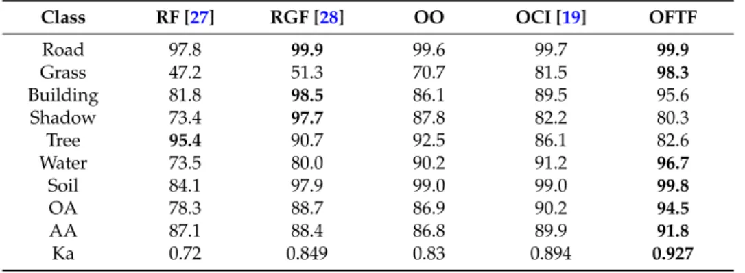
Table 7. Class-specific accuracies (%) for the different approaches in SVM classification of the second UAV image data

Class RF [27] RGF [28] OO OCI [19] OFTF Road 97.8 99.9 99.6 99.7 99.9 Grass 47.2 51.3 70.7 81.5 98.3 Building 81.8 98.5 86.1 89.5 95.6 Shadow 73.4 97.7 87.8 82.2 80.3 Tree 95.4 90.7 92.5 86.1 82.6 Water 73.5 80.0 90.2 91.2 96.7 Soil 84.1 97.9 99.0 99.0 99.8 OA 78.3 88.7 86.9 90.2 94.5 AA 87.1 88.4 86.8 89.9 91.8 Ka 0.72 0.849 0.83 0.894 0.927

Figure 10.Classification results of the different approaches (third UAV image): (a–e) are classification maps based on RF, RGF, original objects, OCI, and the proposed OFTF, respectively.

Table 7.Class-specific accuracies (%) for the different approaches in SVM classification of the second UAV image data.

Class RF [27] RGF [28] OO OCI [19] OFTF

Road 97.8 99.9 99.6 99.7 99.9 Grass 47.2 51.3 70.7 81.5 98.3 Building 81.8 98.5 86.1 89.5 95.6 Shadow 73.4 97.7 87.8 82.2 80.3 Tree 95.4 90.7 92.5 86.1 82.6 Water 73.5 80.0 90.2 91.2 96.7 Soil 84.1 97.9 99.0 99.0 99.8 OA 78.3 88.7 86.9 90.2 94.5 AA 87.1 88.4 86.8 89.9 91.8 Ka 0.72 0.849 0.83 0.894 0.927

(11)

Table 8.Class-specific accuracies (%) of the different approaches in SVM classification of the third UAV image data.

Class RF [27] RGF [28] OO OCI [19] OFTF

Road 55.8 98.6 98.6 98.7 99.2 Grass 73.7 73.9 95.4 91.2 98.6 Building 85.0 80.4 99.4 95.8 99.5 Shadow 92.6 94.6 85.8 86.7 86.5 Tree 54.4 47.3 58.2 77.8 78.4 Water 84.0 74.2 40.8 93.9 98.7 Soil 88.4 90.1 93.9 62.9 59.2 OA 75.9 77.2 89.2 92.8 94.0 AA 75.8 83.7 86.3 89.9 90.6 Ka 0.687 0.711 0.855 0.91 0.92 4. Discussion

In the first experiment, the sensitivity between the relaxing parameter R and the overall accuracy was investigated. As shown in Figure 7, when the value of R ranges from 0.5 to 1.5, the accuracy of the proposed approach increased initially. However, when the value ofRbecame larger than 1.5, the accuracy decreased. In a practical application,Rcan be adjusted and determined in accordance with different images.

In addition, in the first experiment, the adaptability of the proposed OFTF was also investigated with different supervised classifiers. The quantitative results for each classifier are shown in Table4. It can be seen that the proposed OFTF-based classification exhibits the highest accuracy with the SVM classifier. Therefore, SVM was employed as the “classifier” in the second and third experiments.

In the second experiment, the class-specific accuracies for this parameter setup are shown in Table7, and the visual classification map is shown in Figure9. The table and its corresponding classification map show that the proposed OFTF-based approach achieves a higher classification accuracy than the original object-based approach without any filtering process. Furthermore, the proposed OFTF-based approach also obtains a higher classification accuracy than RF [27], RGF [28], and OCI [19] in terms of OA and Ka. In terms of visual performance, the proposed OFTF-based approach is better at smoothing the noise of the classification map when compared to the other approaches. Therefore, the proposed OFTF method can be considered as suitable for improving the performance of VHSR images.

In the third experiment, the specific classification with the different approaches under such a parameter setup is shown in Table8and Figure10. Similar results to those of the second image data were obtained. The proposed OFTF-based classification exhibits the highest accuracy in terms of OA and Ka and provides better visual performance than the other approaches.

Currently, aerial images (including UAV images) are involved in a wide range of remote sensing applications and object-based techniques have been widely applied for VHSR image classification. However, to our best knowledge, although object-based classification methods have been studied extensively, this type of object-based filtering has previously not been proposed. In this study, a novel object-based image filter is proposed to improve the accuracy when applied to aerial images for land cover survey tasks. In addition, it is worth noting that the proposed OFTF is easy to use for applications. It has two parameters:Randiteration. Regarding the optimized relaxing parameter,R can be available by trial-and-error experiments when applied for classification. The other parameter, iteration, can be fixed as a constant, because the proposed OFTF is based on two-fold constraints (topology and features) and a larger iteration will not result in over-smoothing the results. With the rapid development of high resolution remote sensing images (such as aerial and UAV images), this novel object-based filter is significant and may promote more potential applications.

(12)

Remote Sens.2016,8, 1023 12 of 14

The results and discussions reveal that the proposed OFTF is feasible for and effective in reducing the differences among intra-classes. This feature is helpful in improving the performance of VHSR image land cover classification.

5. Conclusions

In this paper, a new approach called OFTF was proposed to improve the performance of VHSR image classification. Experiments were conducted on three real VHSR images to show the effectiveness of the proposed approach. The results of OFTF were better in terms of classification accuracies than those of widely used object-based approaches, i.e., two relatively new methods based on considering contextual spatial information [27,28,31]. The novel contribution of the proposed OFTF approach is three-fold. First, although object-based image analysis approaches have been studied extensively, to the best of our knowledge, the concept of object-based filtering has not been proposed yet. Second, a traditional pixel-wise image filter usually smooths an image through a regular window and it cannot be used directly for smoothing the difference of segmented image objects. Meanwhile, the proposed OFTF provides a novel way to smooth the difference of the target's objects through topology-feature constraints. The procedure of the proposed OFTF is more intuitive and reasonable for various grounded targets because a ground target is usually presented as objects that are spatially contiguous and possess similar features. Third, compared with traditional spatial feature extraction algorithms, the proposed OFTF approach is simple and may imply more potential applications for analysis of VHSR remote sensing images.

In addition to topology, the spatial knowledge implied in the VHSR image is difficult to portray both quantitatively and precisely. Therefore, as a topic for future research, a more comprehensive topology relationship and spatial knowledge, such as azimuth or location, will be extracted from VHSR imagery. In theory, using a more reasonable feature to model the target in the remote sensing image scene results in higher accuracy.

Acknowledgments: The authors would like to thank the editor-in-chief, the anonymous associate editor, and the reviewers for their insightful comments and suggestions. This work was supported by the Key Laboratory for National Geographic Census and Monitoring, National Administration of Surveying, Mapping and Geoinformation (2015NGCM) and the project from the China Postdoctoral Science Foundation (2015M572658XB), and the National Natural Science Foundation of China (61302135).

Author Contributions: Z.L. was primarily responsible for the original idea and experimental design. W.S. provided important suggestions for improving the paper’s quality. J.A.B. provided ideas to improve the quality of the paper. X.N. provided funding for supporting this research and publication.

Conflicts of Interest:The authors declare no conflict of interest. References

1. Huang, X.; Zhang, L. An SVM ensemble approach combining spectral, structural, and semantic features for the classification of high-resolution remotely sensed imagery.IEEE Trans. Geosci. Remote Sens.2013,51, 257–272. [CrossRef]

2. Pu, R.; Landry, S. A comparative analysis of high spatial resolution ikonos and worldview-2 imagery for mapping urban tree species.Remote Sens. Environ.2012,124, 516–533. [CrossRef]

3. Garrity, S.R.; Allen, C.D.; Brumby, S.P.; Gangodagamage, C.; McDowell, N.G.; Cai, D.M. Quantifying tree mortality in a mixed species woodland using multitemporal high spatial resolution satellite imagery. Remote Sens. Environ.2013,129, 54–65. [CrossRef]

4. Li, M.; Ma, L.; Blaschke, T.; Cheng, L.; Tiede, D. A systematic comparison of different object-based classification techniques using high spatial resolution imagery in agricultural environments.Int. J. Appl. Earth Obs. Geoinf.2016,49, 87–98. [CrossRef]

5. Bruzzone, L.; Carlin, L. A multilevel context-based system for classification of very high spatial resolution images.Geosci. IEEE Trans. Geosci. Remote Sens.2006,44, 2587–2600. [CrossRef]

6. Huang, X.; Zhang, L.; Li, P. A multiscale feature fusion approach for classification of very high resolution satellite imagery based on wavelet transform.Int. J. Remote Sens.2008,29, 5923–5941. [CrossRef]

(13)

7. Fauvel, M.; Tarabalka, Y.; Benediktsson, J.A.; Chanussot, J.; Tilton, J.C. Advances in spectral–spatial classification of hyperspectral images.Proc. IEEE2013,101, 652–675. [CrossRef]

8. Ghamisi, P.; Dalla Mura, M.; Benediktsson, J.A. A survey on spectral–spatial classification techniques based on attribute profiles.IEEE Trans. Geosci. Remote Sens.2015,53, 2335–2353. [CrossRef]

9. Zhang, L.; Huang, X.; Huang, B.; Li, P. A pixel shape index coupled with spectral information for classification of high spatial resolution remotely sensed imagery.IEEE Trans. Geosci. Remote Sens.2006,44. [CrossRef] 10. Zhang, H.; Shi, W.; Wang, Y.; Hao, M.; Miao, Z. Classification of very high spatial resolution imagery based

on a new pixel shape feature set.IEEE Geosci. Remote Sens. Lett.2014,11, 940–944. [CrossRef]

11. Dalla Mura, M.; Benediktsson, J.A.; Waske, B.; Bruzzone, L. Morphological attribute profiles for the analysis of very high resolution images.IEEE Trans. Geosci. Remote Sens.2010,48, 3747–3762. [CrossRef]

12. Huang, X.; Guan, X.; Benediktsson, J.A.; Zhang, L.; Li, J.; Plaza, A.; Dalla Mura, M. Multiple morphological profiles from multicomponent-base images for hyperspectral image classification.IEEE J. Sel. Top. Appl. Earth Obs. Remote Sens.2014,7, 4653–4669. [CrossRef]

13. Lv, Z.Y.; Zhang, P.; Benediktsson, J.A.; Shi, W.Z. Morphological profiles based on differently shaped structuring elements for classification of images with very high spatial resolution. IEEE J. Sel. Top. Appl. Earth Obs. Remote Sens.2014,7, 4644–4652. [CrossRef]

14. Falco, N.; Benediktsson, J.A.; Bruzzone, L. Spectral and spatial classification of hyperspectral images based on ica and reduced morphological attribute profiles.IEEE Trans. Geosci. Remote Sens.2015,53, 6223–6240. [CrossRef]

15. Gu, Y.; Liu, T.; Jia, X.; Benediktsson, J.A.; Chanussot, J. Nonlinear multiple kernel learning with multiple-structure-element extended morphological profiles for hyperspectral image classification. IEEE Trans. Geosci. Remote Sens.2016,54, 3235–3247. [CrossRef]

16. Blaschke, T.; Hay, G.J.; Kelly, M.; Lang, S.; Hofmann, P.; Addink, E.; Feitosa, R.Q.; van der Meer, F.; van der Werff, H.; van Coillie, F. Geographic object-based image analysis–towards a new paradigm.ISPRS J. Photogramm. Remote Sens.2014,87, 180–191. [CrossRef] [PubMed]

17. Hussain, E.; Shan, J. Object-based urban land cover classification using rule inheritance over very high-resolution multisensor and multitemporal data.GIScience Remote Sens.2015,53, 164–182. [CrossRef] 18. Malinverni, E.S.; Tassetti, A.N.; Mancini, A.; Zingaretti, P.; Frontoni, E.; Bernardini, A. Hybrid object-based

approach for land use/land cover mapping using high spatial resolution imagery.Int. J. Geogr. Inf. Sci.2011, 25, 1025–1043. [CrossRef]

19. Zhang, P.; Lv, Z.; Shi, W. Object-based spatial feature for classification of very high resolution remote sensing images.IEEE Geosci. Remote Sens. Lett.2013,10, 1572–1576. [CrossRef]

20. Geiss, C.; Taubenbock, H. Object-based postclassification relearning.IEEE Geosci. Remote Sens. Lett.2015,12, 2336–2340. [CrossRef]

21. Dingle Robertson, L.; King, D.J. Comparison of pixel-and object-based classification in land cover change mapping.Int. J. Remote Sens.2011,32, 1505–1529. [CrossRef]

22. Myint, S.W.; Gober, P.; Brazel, A.; Grossman-Clarke, S.; Weng, Q. Per-pixel vs. Object-based classification of urban land cover extraction using high spatial resolution imagery.Remote Sens. Environ.2011,115, 1145–1161. [CrossRef]

23. Farbman, Z.; Fattal, R.; Lischinski, D.; Szeliski, R. Edge-preserving decompositions for multi-scale tone and detail manipulation. In Proceedings of the ACM Transactions on Graphics (TOG), Los Angeles, CA, USA, 11–15 August 2008; p. 67.

24. He, K.; Sun, J.; Tang, X. Guided image filtering. InComputer Vision–ECCV 2010; Springer: Berlin/Heidelberg, Germany, 2010; pp. 1–14.

25. Li, S.; Kang, X.; Hu, J. Image fusion with guided filtering.IEEE Trans. Image Proc.2013,22, 2864–2875. 26. Kang, X.; Li, S.; Benediktsson, J.A. Spectral–spatial hyperspectral image classification with edge-preserving

filtering.IEEE Trans. Geosci. Remote Sens.2014,52, 2666–2677. [CrossRef]

27. Kang, X.; Li, S.; Benediktsson, J.A. Feature extraction of hyperspectral images with image fusion and recursive filtering.IEEE Trans. Geosci. Remote Sens.2014,52, 3742–3752. [CrossRef]

28. Xia, J.; Bombrun, L.; Adalı, T.; Berthoumieu, Y.; Germain, C. Spectral–spatial classification of hyperspectral images using ica and edge-preserving filter via an ensemble strategy.IEEE Trans. Geosci. Remote Sens.2016, 54, 4971–4982. [CrossRef]

(14)

Remote Sens.2016,8, 1023 14 of 14

29. Baatz, M.; Schäpe, A. Multiresolution segmentation: An optimization approach for high quality multi-scale image segmentation.Angew. Geogr. Informationsverarb. XII2000,58, 12–23.

30. Yang, Y.; Li, H.; Han, Y.; Gu, H. High resolution remote sensing image segmentation based on graph theory and fractal net evolution approach. Int. Arch. Photogramm. Remote Sens. Spat. Inf. Sci.2015,40, 197–201. [CrossRef]

31. Xia, J.; Bombrun, L.; Adali, T.; Berthoumieu, Y.; Germain, C. Classification of hyperspectral data with ensemble of subspace ica and edge-preserving filtering. In Proceedings of the 41st IEEE International Conference on Acoustics, Speech and Signal Processing (ICASSP 2016), Shanghai, China, 20–25 March 2016; pp. 1422–1426.

© 2016 by the authors; licensee MDPI, Basel, Switzerland. This article is an open access article distributed under the terms and conditions of the Creative Commons Attribution (CC-BY) license (http://creativecommons.org/licenses/by/4.0/).