Debt Portfolios

DISCUSSION PAPER SERIES

Forschungsinstitut zur Zukunft der Arbeit Institute for the Study of Labor

Debt Portfolios

Debt Portfolios

Thomas Hintermaier

University of Bonn

Winfried Koeniger

Queen Mary, University of London, CEPR and IZA

Discussion Paper No. 5653

April 2011

Any opinions expressed here are those of the author(s) and not those of IZA. Research published in this series may include views on policy, but the institute itself takes no institutional policy positions. The Institute for the Study of Labor (IZA) in Bonn is a local and virtual international research center and a place of communication between science, politics and business. IZA is an independent nonprofit organization supported by Deutsche Post Foundation. The center is associated with the University of Bonn and offers a stimulating research environment through its international network, workshops and conferences, data service, project support, research visits and doctoral program. IZA engages in (i) original and internationally competitive research in all fields of labor economics, (ii) development of policy concepts, and (iii) dissemination of research results and concepts to the interested public. IZA Discussion Papers often represent preliminary work and are circulated to encourage discussion. Citation of such a paper should account for its provisional character. A revised version may be available directly from the author.

IZA Discussion Paper No. 5653 April 2011

ABSTRACT

Debt Portfolios

We provide a model with endogenous portfolios of secured and unsecured household debt. Secured debt is collateralized by owner-occupied housing whereas unsecured debt can be discharged according to bankruptcy regulations. We show that the calibrated model matches important quantitative characteristics of observed wealth and debt portfolios for prime-age consumers in the U.S. We then establish the quantitative result that home equity does not serve as informal collateral for unsecured debt since, as in the data, unsecured debtors hold small amounts of home equity in equilibrium. Thus, observed variations in homestead exemptions, which are an important part of U.S. bankruptcy regulation, have a small effect on the quantity and price of unsecured debt.

JEL Classification: E21, D91

Keywords: household debt portfolios, housing, collateral, bankruptcy, commitment, income risk

Corresponding author: Winfried Koeniger

School of Economics and Finance Queen Mary, University of London Mile End Road

London, E1 4NS United Kingdom

E-mail: [email protected]

*

This is a substantially revised version of our analysis of U.S. consumer debt previously circulated with the working titles “Income Risk, Risk Sharing and Household Debt” or “Income Risk, Durables and Collateral Loans.” We thank participants of various seminars and conferences for helpful comments. Part of this research has been conducted while Thomas Hintermaier was a Max Weber Fellow at the

1

Introduction

Household debt is sizeable and has increased substantially in the last decades in the U.S., the UK and most other European countries. The aggregate debt level hides substantial di¤erences between debt types and their composition on the balance sheets of individual households. Most household debt is secured by housing collateral whereas some debt is un-secured and can be written o¤ in bankruptcy procedures in the U.S., the UK and some, but not all, European countries.1 _{Interestingly, portfolios of these debt types di¤er}

substan-tially across households (see Section 2). In this paper we present a model which allows for heterogeneity across households and generates such debt portfolios endogenously.

The key new feature in our model is housing which allows for a meaningful distinction between secured and unsecured debt and thus permits us to analyze debt portfolios. We obtain heterogeneity in debt portfolios by modeling consumer choices over the life cycle, as-suming uncertain labor income and incomplete markets. Consumers then cannot fully insure the labor-income risk and hold di¤erent portfolios depending on their age and histories of shocks. Micro-founded heterogeneous-agent models with these characteristics have been pio-neered by Deaton (1991), Aiyagari (1994) and Carroll (1997) and have attracted substantial attention in recent years.

We …nd that our calibrated model matches well important cross-sectional characteristics of wealth and debt portfolios in the U.S. Against this background, we establish the following quantitative results. Unsecured debtors hold small amounts of home equity in the equilibrium of the calibrated model, as in the data. Thus, home equity does not provide informal collateral for unsecured debt and hence does not mitigate the limited commitment problem resulting from the bankruptcy option. This result has important implications for bankruptcy regulation. Equilibrium pricing of unsecured debt and the associated portfolio choices imply that homestead exemptions, which are an important part of U.S. bankruptcy regulation, have a quantitatively small e¤ect. Regulation could a¤ect the quantity and price of unsecured debt only if the size of the exemptions is very small (less than a tenth of annual labor earnings). This …nding is in contrast to results in Pavan (2008), who did not explicitly

1_{See Dynan and Kohn (2007), Tudela and Young (2005), Jentzsch and San José Riestra (2006) and their}

distinguish between secured and unsecured debt, but is consistent with the inconclusive empirical evidence on the e¤ect of homestead exemptions on debt and bankruptcy incidence (see, for example, the survey in White, 2006).

Our paper relates to recent research by Athreya (2002), Chatterjee, Corbae, Nakajima and Ríos-Rull (2007) and Livshits, MacGee and Tertilt (2007) who have extended the classic heterogeneous-agent models to analyze unsecured debt. Importantly, these models assume that consumers only have access to unsecured debt. In this paper we relax this assumption and allow for an endogenous debt portfolio: consumers can take on secured debt such as mortgages, which are collateralized by housing, and unsecured debt like credit-card debt. To the best of our knowledge only Athreya (2006) attempts to distinguish secured and unsecured debt but does not model housing wealth. In his model the amount of collateral is exogenous whereas consumers in our model endogenously accumulate housing collateral which also generates utility. This modeling of durables like housing is closest to Fernández-Villaverde and Krueger (forthcoming), Kiyotaki, Michaelides and Nikolov (2011) and Yang (2009) who, however, do not allow for equilibrium bankruptcy and unsecured debt.2

The main contribution of our paper is that we explicitly model debt portfolios. The advantages of analyzing housing wealth, secured and unsecured debt simultaneously are at least threefold. The …rst advantage is that the model has an additional margin of substitu-tion in the debt portfolio, between secured and unsecured debt. That margin adds realism by capturing the two types of debt which are relevant in consumer …nance. The margin also gives households the choice to provide informal collateral for unsecured debt by holding home equity above the amount which is exempt in bankruptcy procedures. This is particularly im-portant when one investigates the supply-side e¤ects of the limited commitment introduced by the bankruptcy option. We will show how the joint analysis of housing wealth, secured and unsecured debt in our quantitative framework generates new insights for the e¤ect of homestead exemptions on the equilibrium price and quantity of unsecured debt.

The second advantage is more realism in a key aspect of the analysis since most of consumers’total debt holdings in the data are secured by housing collateral. Thus, a quan-titative model of household debt needs to explain not only the rather small unsecured debt

2_{See also Yao and Zhang (2005) for an analysis of housing and portfolio choice and Mankart and Rodano}

position but the whole debt portfolio. In our model the optimal choices for these portfolios are constrained by endogenous debt limits for unsecured and secured debt. This is also important for the predictions of the model concerning consumer bankruptcy because only unsecured debt can be discharged by …ling for bankruptcy.

The third advantage is that the explicit modeling of housing introduces an endogenous bankruptcy cost which has been neglected in previous quantitative research. Upon seizure of owner-occupied housing, the home equity above the amount exempt in bankruptcy pro-cedures is used to satisfy unsecured creditors’ claims. Since adjusting the housing stock is costly, the cost of bankruptcy depends on the size of a consumer’s housing wealth and secured debt.

The rest of this paper is structured as follows. In Section 2 we present empirical facts which are instructive for our analysis. We present the model in Section 3, followed by its numerical solution and calibration in Section 4. In Section 5 we analyze the role of home equity as informal collateral and the implications for bankruptcy regulation. We then conclude in Section 6.

2

Empirical facts

In this section we summarize the empirical facts on wealth and debt portfolios which are relevant for the quantitative application of our model. We then brie‡y review the key features of U.S. consumer bankruptcy regulation which the model shall capture.

2.1

Data

We use the Survey of Consumer Finances (SCF) to present facts on wealth and debt portfolios of U.S. consumers. The SCF has been widely used as it provides the most accurate infor-mation on consumer …nances in the U.S. (see Kennickell, 2003, and the references therein). We focus on the SCF 2004 to calibrate our model since, for the purposes of our analysis, it is representative of the three waves of the SCF in the 2000s. We prefer the SCF 2004 to the most recent SCF 2007 for the calibration since the 2007 SCF wave contains data from interviews between May 2007 and March 2008 that are likely to be in‡uenced by the start

of the …nancial crisis.

We largely follow Budría Rodríguez, Díaz-Giménez, Quadrini and Ríos-Rull (2002) and Díaz-Giménez, Quadrini and Ríos-Rull (1997) in constructing measures for wealth and labor earnings in the U.S. We account for di¤erences in household size using the equivalence scale reported in Fernández-Villaverde and Krueger (2007), Table 1, last column, with a weight of 1 for the …rst person in the household, 0.34 for the second person and approximately 0.3 for each additional member of the household. To make the empirical data comparable with the data generated by the model, we normalize all variables by average net labor earnings in the whole sample.3 _{More precisely, we use SCF data on gross labor earnings and the}

NBER tax simulator described in Feenberg and Coutts (1993) to construct a measure for disposable labor earnings after taxes and transfers for each household. Arguably, after-tax rather than pre-tax earnings matter for households’ consumption and portfolio decisions since some uninsurable labor earnings risk may be eliminated by redistributive taxes and transfers. More detailed information on the de…nition of the variables and the sample is contained in the data appendix.

We focus on empirical facts for prime-age households with a head between ages 26 and 55. As Livshits et al. (2007), our model abstracts from death before age 76 and there-fore this is a good approximation of the data only up to a certain age. Life tables for the U.S. show that 90% of those born alive are still alive at age 55 and then have an av-erage life expectancy of another 25 years (see the National Center of Health Statistics at http://www.cdc.gov/nchs/products/life_tables.htm). Allowing for a positive probability of death at all stages of the life cycle would unnecessarily increase the computational burden further and since debt portfolios are most relevant early in the life cycle, as we will see below, this simpli…cation of our analysis seems not very restrictive.4

Since the questions in the SCF survey refer to income in the previous year and agents have made their consumption and portfolio choices conditional on this income, we interpret the SCF asset data as end-of-period information at the time when the survey is carried out.

3_{When computing the statistics in the data, we use the sampling weights provided in the SCF.}

4_{Allowing for a positive probability of death and assuming accidental bequests, for example, would add a}

…xed-point problem in our numerical solution. This would be very costly given the substantial computational burden of our model.

2000s 2004 2004: 90th

net worth pctile

(1) (2) (3)

Wealth

Housing wealth (primary residence) 3.38 3.48 2.50

+ Net-…nancial assets 4.07 3.69 -0.01

= Total net worth (fraction of average net lab. earnings) 7.45 7.17 2.49

Financial assets

Financial assets 4.714 4.407 0.773

+ Secured debt -0.610 -0.688 -0.746

+ Unsecured debt -0.031 -0.033 -0.037

= Net-…nancial assets (fraction of average net lab. earnings) 4.073 3.686 -0.010

Debt

Secured debt (in % of total secured + unsecured debt above) 95.16 95.42 95.27 Home ownership (in % of sample size) 66.91 67.43 64.40 Bankrupt in previous year (in % of sample size) 1.42 1.53 1.67

Table 1: Wealth and debt portfolios of households with a head between ages 26 and 55. Sample means of cross-sections in the 2000s (2001-2007) and 2004, respectively. Means in column (3) are computed for households up to the 90th percentile of the net worth distrib-ution. Source: Authors’calculation based on the SCF. Notes: Quantities are normalized by average net labor earnings of the whole sample in the respective sample year.

2.2

Wealth and debt portfolios

Table 1 displays the means of wealth and debt for prime-age households denominated in average net labor earnings in the respective survey year. Column (1) displays the average of the means across the SCF surveys in the 2000s (the SCF 2001, 2004 and 2007) whereas column (2) shows these averages only for the SCF 2004. The sample means are very similar in both columns of Table 1. We thus focus on the SCF 2004, the last SCF wave before the …nancial crisis, when we calibrate our model which is not designed for analyzing such an extreme event.

For the calibration we further restrict the sample to consumers up to the 90th percentile of the net worth distribution. The reason is that, as is well known, standard incomplete-market models cannot match the substantial wealth holdings in the top decile of the wealth distribution (see, for example, Hintermaier and Koeniger, 2011, and the references therein). If such a model were calibrated to match average wealth in the whole sample, the model

would predict that consumers up to the 90th percentile hold too much wealth compared with the data. Such a prediction bias is particularly undesirable given that the focus of this paper is on debt portfolios. Table, column (3) shows that while the wealth holdings are obviously smaller for consumers below the 90th percentile of the net worth distribution, most of the other statistics are quite similar. The main di¤erence is the much smaller …nancial asset position compared with column (2). Such assets are held mostly by consumers in the top decile of the net worth distribution.

Table 1, column (3) shows that average wealth of prime-age households below the 90th percentile of the net worth distribution consists mostly of owner-occupied housing wealth (for the primary residence). 64% of households own a home which can be used as collateral to secure debt in real-life debt contracts. Secured debt accounts for 95% of the debt.5 _As

to the incidence of debt, 46% of prime-age households below the 90th percentile of the net worth distribution hold some debt, 39% hold secured debt and 13% hold unsecured debt. Unsecured debt can be written o¤ in bankruptcy procedures and 1.6% of the households have made use of that option in the year previous to the survey date.

Since an important dimension of heterogeneity in our life-cycle model is age, Figures 1 and 2 illustrate how wealth and debt portfolios change with age in the SCF cross-section up to the 90th percentile of the net worth distribution.6 _{Figure 1 shows that young consumers}

start their life with very little equity, borrowing against their housing collateral. Figure 2 shows that most of the debt is secured and unsecured debt is mainly taken on by young consumers. By their mid-thirties consumers, on average, reduce their debt and accumulate signi…cant amounts of other equity (see Fernández-Villaverde and Krueger, forthcoming, who document similar patterns of …nancial assets and durables in the SCF 1995).

The data in the SCF also reveal some important patterns of di¤erence between consumers with and without unsecured debt, which we would like to capture with our model. Households with unsecured debt are younger and have smaller labor earnings than the sample mean. Moreover, they own less housing wealth while holding more secured debt than the rest of

5_{Constructing model counterparts for secured and unsecured debt in the data is not trivial. We refer to}

the data appendix for details.

6_{We explain below how we compare the data cross-sections with the life-cycle pro…les generated by the}

model. To obtain the age cross-sections displayed in the …gures, we divide the range between ages 23 and 76 into 18 three-year age groups as in the model. We then compute the averages for each of these age groups.

0 1 2 3 4 A v er age l a bor -ea rni ng equ iv a len ts 27 30 33 36 39 42 45 48 51 54 Age Average of SCF 2001, 2004, 2007 0 1 2 3 4 A v er age l a bor -ea rni ng equ iv a len ts 27 30 33 36 39 42 45 48 51 54 Age SCF 2004

Housing wealth (primary residence) Home equity Other equity

Figure 1: Average portfolios of consumers between ages 26 and 55 up to 90th percentile of the net worth distribution in the 2000s. Source: Authors’calculations based on the Survey of Consumer Finances (SCF). See the data appendix for variable de…nitions. Notes: The unit is the average of net labor earnings in the whole SCF sample. The axis labeling for age uses the midpoint of the age interval in the respective three-year age group. The graph plots the average for each age group.

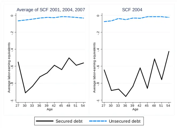
0 -.2 -.4 -.6 -.8 -1 A v er age l a bor -ea rni ng equ iv a len ts 27 30 33 36 39 42 45 48 51 54 Age Average of SCF 2001, 2004, 2007 0 -.2 -.4 -.6 -.8 -1 A v er age l a bor -ea rni ng equ iv a len ts 27 30 33 36 39 42 45 48 51 54 Age SCF 2004

Secured debt Unsecured debt

Figure 2: Average debt portfolio of consumers between ages 26 and 55 up to 90th percentile of the net worth distribution in the 2000s. Source: Authors’calculations based on the Survey of Consumer Finances (SCF). See the data appendix for variable de…nitions. Notes: The unit is the average of net labor earnings in the whole SCF sample. The axis labeling for age uses the midpoint of the age interval in the respective three-year age group. The graph plots the average for each age group.

the sample. Thus consumers with unsecured debt have less home equity than the rest of the sample.

2.3

U.S. consumer bankruptcy

The regulation for consumer bankruptcy in the U.S., relevant for the SCF 2004, is the Federal Bankruptcy Act of 1978. This act contains two Chapters for non-farming households. Consumers can choose to …le for personal bankruptcy under either Chapter 7 or Chapter 13. The main features of these two Chapters, which are important for our analysis, can be summarized as follows (see Sullivan et al., 1999, for further details).

Under Chapter 7 of the bankruptcy act, the debtor can write o¤ his unsecured debts but must surrender all his assets except for speci…ed exempt amounts. Most of the bankruptcy exemptions are speci…ed as homestead exemptions (see, for example, Grant and Koeniger, 2009). Secured debt is senior and has to be honored, however, so that bankruptcy exemptions only apply to the home equity which remains after servicing secured credit claims.7

Under Chapter 13, the debtor agrees to a repayment schedule for part or all of the debt and retains his assets. The repayment plan usually is speci…ed for three years but can take up to …ve years. Importantly, the debtor cannot repay less under Chapter 13 than what creditors would get paid under Chapter 7. Hence, we focus on Chapter 7 in our model since it places a lower bound on the unsecured-debt claims of the creditors. This is not a strong restriction since most consumers who …le for bankruptcy do so under Chapter 7 (70%) and many of the repayment plans initiated under Chapter 13 fail and are later converted into Chapter 7. If consumers …le for bankruptcy under Chapter 7, they are not allowed to …le for bankruptcy again within the next six years (see Sullivan et al., 1999).

The main reason for consumer bankruptcy, identi…ed by Sullivan et al. (2000), is earnings risk. Two thirds of the bankrupt consumers mention job related problems like wage cuts or unemployment. A …fth of bankrupt consumers reports health problems (multiple responses were permitted) where in 60% of these cases the implied income losses due to missed

work-7_{Our model abstracts from house price risk and negative home equity so that we do not discuss the}

regulation on mortgage foreclosures and bankruptcy. Data on charge-o¤ and delinquency rates by the Federal Reserve at http://www.federalreserve.gov/releases/chargeo¤/ show that real-estate loans have been essentially secure before 2007 with charge-o¤ and delinquency rates of less than a tenth of those of other consumer loans.

days, demotion or lost jobs are mentioned as the reason for bankruptcy. Therefore we focus on labor earnings shocks as a reason for bankruptcy in this paper.8 Having presented the key relevant facts, we are now ready to set up the model.

3

The model

We build on the life-cycle model of unsecured debt by Livshits et al. (2007). We assume that the economy is populated by a large number of consumers, indexed by i, who live for

J = 18 periods, where each period j has a length of three years. Life begins at age 23 and the …rst 14 periods (until age 65) are working periods in which people receive income shocks. In the last four periods consumers are in retirement and face no uncertainty. Life ends after age 76. Below we drop the index i for di¤erent consumers to simplify notation unless the distinction between consumers is particularly important.

Preferences. Consumers maximize expected lifetime utility. Utility is derived from a consumption basket (cj; fj)which is non-separable in non-durable consumption cj and the service ‡owfj from housing. We assume that one unit of the housing stock, whether rented or owned, provides units of this service ‡ow. For the quantitative application of the model we assume recursive utility since we want to have ‡exibility in the calibration concerning the strength of the intratemporal and intertemporal consumption smoothing motive. The utility is speci…ed as Uj = h (cj; fj)1 + E Uj1+1 1 1 i 1 1 ,

with expectation operatorE, discount factor , risk aversion 0, intertemporal elasticity of substitution 1= 0and

(cj; fj) = (cj) fj+f

1

.

8_{We abstract from medical expense shocks to contain the computational burden of our model with housing}

as an additional endogenous state variable. See Chatterjee et al. (2007) or Livshits et al. (2007) for models with health expense shocks.

The parameter = 1 if the consumer owns housing and = r _{with 0} r _{1 if the} consumer rents. As is common in the literature, the parameter r allows us to capture foregone utility of renters, for example due to hold-up problems which are left unmodelled. We call r _{rental e¢ ciency.}

The speci…cation of preferences implies that the demand for housing service ‡ows may be zero since consumers then rely on the constant autonomous level of the service ‡ow f >0, which is assumed to be small and positive. Furthermore, consumers prefer an early resolution of uncertainty if >1= , as will be the case in our calibration.

Our parametric assumptions about preferences encompass many of the previous numerical applications which we are aware of. The preferences would simplify to the standard CRRA case if = . Moreover, the Cobb-Douglas consumption basket is in line with empirical evidence on the substitutability between housing and non-durables (see Davis and Ortalo-Magné, 2011, and Fernández-Villaverde and Krueger, forthcoming, for further discussion and references).

Labor earnings. The log of labor earnings of consumeri at age j is given by

lnyij = j +zij,

where j is the deterministic labor endowment of the household with age 23 + 3(j 1) at the beginning of period j. The endowment j is hump-shaped over the life cycle and zij is a persistent income shock.

Assets and market arrangements. The stock of housing that creates the service ‡ow of utility can be either rented or owned. We denote the owned housing wealth by h. Owned housing can be used as collateral to secure debt but can only be adjusted at a cost. Alter-natively, housing can be rented at a price determined by a no-arbitrage condition. The price of renting one unit of housing equals the user cost ra_{+ , where r}a _{is the risk-free interest} rate on …nancial assets and is the rate at which housing depreciates.9

9_{As in Gervais (2002), we implicitly assume that …nancial institutions take on deposits and purchase}

Consumers hold portfolios of secured debt as _{0, unsecured debt a}u _{< 0, risk-free} …nancial assets au 0 and owned housing wealth h. Secured debt is backed by owner-occupied housing as collateral and bears an interest raters_{. Risk-free …nancial assetsa}u ₀ earn interest ra_{. We assume that there is a borrowing spread, r}s _{> r}a_{, due to a cost of} …nancial intermediation. We further assume that the cost of intermediation is larger for unsecured debt so that the interest rate for unsecured debt is at least ru _{> r}s _{> r}a_{. As we} discuss further when we calibrate the model, this is a common assumption which is realistic. Unsecured debt au _{<0 is not backed by collateral and we allow consumers to discharge} unsecured debt in bankruptcy procedures. Since creditors price the possibility of bankruptcy, the interest rate on unsecured debt consists of the base rate ru _{and an endogenous risk} premium. We present the pricing of unsecured debt by …nancial intermediaries in detail below.

Adjustment costs. Whereas …nancial assetsas _{and a}u _{can be adjusted costlessly by the} consumer, we assume that the adjustment of owned housingh is costly. These costs can be thought of as fees for real estate agents and generate realistic lumpy investment patterns for housing. Moreover, it sharpens the distinction between owner-occupied housing and non-durables in our model as adjustment costs are one key di¤erence between these two types of goods. Similar to Díaz and Luengo-Prado (2008), we specify the costs as

(h_j+1; hj) = 8 > > > < > > > : c+_fhj if hj+1 > hj 0 if (1 )hj hj+1 hj c_fhj if hj+1 <(1 )hj ,

where the adjustment cost is allowed to be asymmetric in the direction of adjustment. We attach asterisks to the portfolio choices to distinguish them from realizations after bank-ruptcy choice. Note that in our speci…cation of the adjustment cost function there is an interval of choices h_j+1 for which no adjustment costs need to be paid. The end points of this interval are the levels of housing if it depreciates and if it is fully maintained.10

10_{The numerical solution of the model will require discretization of choices. The above speci…cation is}

State variables and the timing of choices. Each consumer enters the period with the pair of endogenous state variables, net-…nancial assets aj asj +auj and owned housinghj. Two exogenous state variables are also relevant to the decision problem. These consist of the state of current income yj and of a moving indicator mj. This exogenous moving indicator determines if a consumer has to rent or if he can choose between either renting or owning the home. As in Díaz and Luengo-Prado (2008), a plausible calibration of exogenous variation in this moving indicator helps to capture realistic patterns of home ownership over the life cycle.

Given the endogenous and exogenous states the consumer chooses consumption and the asset portfolio. The asset returns accrue and the consumer enjoys utility before the new realizations of the exogenous state variables, yj+1 and mj+1, are drawn. The consumer

then decides whether to declare bankruptcy. The law of motion of the pair of endogenous state variables, aj+1 and hj+1 that enter the decision problem next period, depends on the

bankruptcy choice. We now characterize the constraints for the consumer choices and the bankruptcy procedure in more detail before we formulate the recursive problem.

Collateral constraint. The amount of secured debt of the consumer is bounded by the collateral constraint. Only owned housing net of adjustment costs can be used as collateral to secure debt so that we specify the collateral constraint as

as_j+1 min( ;1 c_f)h_j+1 , (1)

where is the exogenous maximum loan-to-value ratio imposed by the …nancial regulator. If < 1 c_f, the access to secured debt is more constrained than necessary to guarantee repayment in the presence of adjustment costs.

Budget constraint. If the consumer is hit by a moving shock, mj = 1, the consumer cannot own a home and thus cannot hold secured debt so thatas

j+1 =hj+1 = 0. The budget

constraint for a renter is

where the price qu_j( _j+1; yj; Bj) = 8 < : (1 +ra₎ 1 _{if a}u j+1 0 1 +ru j( j+1; yj; Bj) 1 if au j+1 <0 .

If the consumer holds unsecured debt, au

j+1 < 0, the price depends on the portfolio j+1

(as

j+1; auj+1; hj+1), the exogenous state of current incomeyj and the bankruptcy ‡agBj which equals 1 if the consumer has declared bankruptcy in the previous period and 0 otherwise. Since the moving shock is idiosyncratic and, unlike the income shock, not persistent, the price

qu

j( j+1; yj; Bj)does not depend explicitly on the exogenous statemj. The moving indicator mj a¤ects prices, however, through the restrictions which it imposes on the portfolio choices

j+1. We discuss the pricing of unsecured debt further below.

If mj = 1, the consumer can spend resources aj +hj +yj on non-durable consumption cj, the …nancial asset auj+1 and housing rentalfj, whereqh = 1=(1 ). Since the consumer has to divest the housing stock, adjustment costs are (0; hj).

If mj = 0, the consumer can choose between renting and owning. If the consumer rents, the budget constraint is as in (2). If the consumer owns, the budget constraint is:

q_jsas_j+1+qu_j( _j+1; yj; Bj)auj+1+q

h_h

j+1+ (hj+1; hj) +cj aj +hj+yj , (3) where the expenditure on housing is qh_h

j+1. In this case the owned housing wealth hj+1

creates a service ‡ow fj =hj+1 and can be used as collateral for secured debt asj+1 0with

a price qs

j = 1=(1 +rs).

Bankruptcy. At the time of bankruptcy …ling the consumer is obliged by law to reveal his …nancial status to the bankruptcy judge. In particular, the judge knows the amount of the owned housing wealthh_j+1 and the composition of …nancial debtas

j+1 and auj+1. Ifauj+1 0,

the consumer has no unsecured debt which can be written o¤ and bankruptcy is not an option. The interesting case is when au

j+1 < 0. Since secured debt asj+1 has priority and

needs to be paid irrespective of speci…ed home exemption levels, the bankruptcy judge …rst computes the amount of the owned housing wealth that remains after repaying all secured debt. Note that for rentersh_j+1 =as

unsecured debt is

hleft for unsecured = (1 c_f)h_j+1+as_j+1 .

The judge then determines the maximum amount which could be divested from the remaining housing wealth, given the exemption level hy _{speci…ed in the bankruptcy regulation. That}

amount is

max net divestment _{= max h}left for unsecured _hy_{;0 .}

The housing wealth used to repay unsecured debt is then equal to that maximum amount or less if the outstanding amount of unsecured debt is smaller:

hto unsecured = min max net divestment; au_j+1 .

As speci…ed in the U.S. bankruptcy law, the judge only sells the home if some of the home equity can be used to repay unsecured debt. Thus, the housing wealth which remains for the consumer after the bankruptcy procedure is

hB =

8 < :

hleft for unsecured _hto unsecured _if max net divestment _<0

h_j+1 if max net divestment _{= 0} ,

and net-…nancial assets are

aB =

8 < :

0 if max net divestment <0

as

j+1 if max net divestment = 0

where the consumer starts afresh without unsecured debt. The evolution of the assets can thus be summarized as

hj+1 = 8 < : h_j+1 if no bankruptcy hB(as_j+1; au_j+1; h_j+1) if bankruptcy , (4) aj+1 = 8 < : a_j+1 as j+1+auj+1 if no bankruptcy aB(as_j+1; au_j+1; h_j+1) if bankruptcy . (5)

The pricing of unsecured debt. The price of unsecured debt is determined by perfectly competitive …nancial intermediaries which observe current income yj, the portfolio j+1

(as

j+1; auj+1; hj+1), the bankruptcy ‡ag Bj and the age j of the consumer. As mentioned above, the price qu

j( j+1; yj; Bj) does not depend explicitly on the exogenous state mj since the moving shock is idiosyncratic and not persistent as the income shock.

The intermediaries price unsecured debt forming expectations about the draws of future income, the moving shock and the implied probability of bankruptcy. There is no cross-subsidization across consumers so that consumers with di¤erent portfolios, age or income state may receive a di¤erent interest quote.

De…ning the probability of bankruptcy as j( j+1; yj; Bj), the zero-pro…t condition implies that the price for unsecured debt is given by

q_ju( _j+1; yj; Bj) = 1 j( j+1; yj; Bj) qu (6) + j( j+1; yj; Bj)qu hto unsecured( _j+1) au j+1 ,

where qu _{= 1=(1+r}u_{). If the probability of bankruptcy is zero,}

j( j+1; yj; Bj) = 0, or if no unsecured debt is discharged when a consumer …les,hto unsecured( _j+1) = au_j+1 , then the risk premium on unsecured debt is zero: qu

j( j+1; yj; Bj) =qu. The probability of bankruptcy is zero, for example, if the consumer has declared bankruptcy in the previous period so that

Bj = 1.

The recursive formulation with optimal default. The decision problems of a con-sumer depend on the moving shock mj and on the bankruptcy decision in the previous period. Being hit by a moving shock (mj = 1) implies the restriction on portfolio choice h_j+1 = as

j+1 = 0. Having declared bankruptcy in the previous period restricts the

bank-ruptcy choice. This is consistent with the U.S. bankbank-ruptcy law which forbids consumers to …le for bankruptcy within six years after a previous bankruptcy procedure. Since a period has a length of three years in our model, we assume that no bankruptcy can be declared for one period.

If the consumer is not hit by a moving shock, mj = 0, he can choose whether to own or to rent housing. The value function

Vj(aj; hj; yj) = max Vjr(aj; hj; yj); Vjo(aj; hj; yj) denotes the envelope of the value function when renting,Vr

j(aj; hj; yj), and the value function when owning the home, Vo

j (aj; hj; yj). The value function V_jB(aj; hj; yj) = max h V_jr;B(aj; hj; yj); V o;B j (aj; hj; yj) i

denotes the envelope of the value functions for rentingV_jr;B(aj; hj; yj)and owningVjo;B(aj; hj; yj) if the consumer has declared bankruptcy in the previous period. If the consumer is hit by a moving shock,mj = 1, he cannot own the home and only the value functionsVjr(aj; hj; yj)and V_jr;B(aj; hj; yj) determine his optimal choices. We now specify how the value functions Vr

j (aj; hj; yj), Vjr;B(aj; hj; yj),Vjo(aj; hj; yj)and Vjo;B(aj; hj; yj) are obtained.

Let !j denote the probability of a moving shock mj = 1 at age j. The value of renting is Vr

j if no bankruptcy has been declared in the previous period:

V_jr(aj; hj; yj) = (7) max au j+1;fj (aj +hj +yj qju( j+1; yj;0)auj+1 (r a_{+ )q}h_f j (0; hj) | {z } cj ; fj)1 + !j+1E max Bj+1 [V_jr₊₁(a_j+1;0; yj+1);(1 )Vjr;B+1(0;0; yj+1)]1 +(1 !j+1)E max Bj+1 [Vj+1(aj+1;0; yj+1);(1 )VjB+1(0;0; yj+1)]1 1 1 1 1 , subject to(2),

where E is the expectation operator and 0 1 is an exogenous utility cost of bankruptcy. This can be interpreted as psychological pain or stigma (see Athreya, 2004).11

11_{In Athreya (2004) a penalty 0is subtracted from the value function. With recursive preferences we}

let0 1enter multiplicatively to ensure that the maximum value, computed in the expectation in (7), is positive.

The value of renting is V_jr;B if bankruptcy has been declared in the previous period: V_jr;B(aj; hj; yj) = (8) max au j+1;fj (aj +hj +yj qju( j+1; yj;1)auj+1 (r a_{+ )q}h_f j (0; hj) | {z } cj ; fj)1 + !j+1E Vjr+1(aj+1;0; yj+1)1 +(1 !j+1)E Vj+1(aj+1;0; yj+1)1 1 1 1 1 , subject to(2).

Note that this type of consumer no longer has the option to declare bankruptcy in the current period.

Recalling that fj =hj+1 for owners, the value of owning is Vjo if no bankruptcy has been declared in the previous period:

V_jo(aj; hj; yj) = (9) max as j+1;auj+1;hj+1 (aj +yj+hj qsja s j+1 q u j( j+1; yj;0)auj+1 q h_h j+1 (hj+1; hj) | {z } cj ; h_j+1)1 + !j+1E max Bj+1 [V_jr₊₁(a_j+1; h_j+1; yj+1);(1 )Vjr;B+1(a B_{; h}B_{; y} j+1)]1 +(1 !j+1)E max Bj+1 [Vj+1(aj+1; hj+1; yj+1);(1 )VjB+1(a B_{; h}B_{; y} j+1)]1 1 1 1 1 , subject to (1) and (3).

V_jo;B(aj; hj; yj) = (10) max as j+1;auj+1;hj+1 (aj +yj +hj qsja s j+1 q u j( j+1; yj;1)auj+1 q h_h j+1 (hj+1; hj) | {z } cj ; h_j+1)1 + !j+1E Vjr+1(aj+1; hj+1; yj+1)1 +(1 !j+1)E Vj+1(aj+1; hj+1; yj+1)1 1 1 1 1 , subject to (1) and (3).

Note that the decision problem of the owner contains the collateral constraint (1). Equations (7) and (9) show that the costs of bankruptcy are di¤erent for owners and renters. Both renters and owners are excluded from the option to declare bankruptcy and face an exogenous utility cost of bankruptcy . In addition, owners have to pay adjustment costs for forced home sales in the bankruptcy procedure, in situations where the housing stock after repaying secured debt exceeds the bankruptcy exemption, hleft for unsecured _{> h}y_.

The magnitude of the endogenous bankruptcy cost depends on the size of the owned house and is relevant for our later analysis of home equity as informal collateral and repayment commitment.

Equations (8) and (10) illustrate that we do not assume that consumers are excluded from credit markets after bankruptcy. This assumption is often imposed in models with unsecured debt to make bankruptcy costly enough. Since we have endogenous bankruptcy costs related to owned housing and the exclusion from the option to declare bankruptcy, we do not need this assumption which is at odds with empirical evidence on consumer borrowing after bankruptcy procedures.

Equilibrium de…nition. A recursive competitive equilibrium is characterized by the pol-icy functions for non-durable consumption, the portfolio choices and optimal default so that for given prices {ra; rs} of risk-free assets and secured debt:

value ifmj = 0, and the envelope of value functionsVjr(aj; hj; yj) and Vjr;B(aj; hj; yj) attains its maximal value if mj = 1.

(ii) the pricing scheme for unsecured debtqu

j( j+1; yj; Bj)satis…es the zero-pro…t condition (6), with default probabilities j( j+1; yj; Bj) being determined by optimal default.

Having presented the model and its recursive formulation we now solve the model nu-merically and calibrate it to match wealth and debt portfolios in the U.S.

4

Calibration and numerical results

The discrete choice in the bankruptcy decision and the presence of non-convex adjustment costs imply that we cannot use numerical algorithms for the constrained portfolio choice prob-lem which rely on the di¤erentiability of the value function as in Hintermaier and Koeniger (2010). Thus, we discretize portfolio choices and specify an equi-spaced grid foras

2[ 7:5; 0]

andau ₂[ 3; 0], with a distance between gridpoints of0:22in terms of annual average labor earnings. Forau

2[0; 90] we choose the same grid …neness at0but let the distance between gridpoints increase linearly for larger values ofau in order to economize on computation time. This results in 35 and 54 gridpoints for as _{and a}u_{, respectively. Choosing equi-spaced grids} for debt as < 0 and au < 0 ensures that consumers remain on the grid of possible values for the endogenous state variable a = as_{+ a}u _{with 88 gridpoints where a}

2 [ 7:5; 90]. We then specify the grid for the second endogenous state variableh₂[0; 45]with 148 gridpoints where the grid for his chosen to include the bankruptcy exemption value hy _{and the values}

of h implied by the grid for secured debt as at the collateral constraint (1).12 We check that, for the speci…ed grid, among the feasible housing choices there are choices for which no adjustment costs are incurred. We make sure that widening the bounds of the grid further does not a¤ect the results. Finally, the benchmark calibration allows for 5 Markov states

12_{The grid for the rental choices is speci…ed identically. We have checked that the results for the benchmark}

calibration are robust if we increase the number of gridpoints to 71 gridpoints foras_{, 113 gridpoints fora}u_,

with a distance between gridpoints of 0:11 in terms of annual average labor earnings, resulting in 183 gridpoints foraand 184 gridpoints for h. Due to the curse of dimensioniality, resulting both from a larger state space and choice set, computing time increased roughly by factor 10.

of the stochastic component of labor earnings, while we have checked the robustness of our benchmark results for 11 Markov states.

Since solving the model takes 13 hours on a PC of the current computing vintage using Fortran code, we do not perform a full grid search over the whole parameter space in our calibration. We solve the model in some regions of the parameter space, which we consider plausible, and then use the interpolation method of Kriging to check whether we can improve the model predictions in other parts of the parameter space.

Kriging is a geostatistical technique which, under certain assumptions, computes the best linear unbiased prediction for target statistics via interpolation on the parameter space and is closely related to regression analysis.13 _{Kriging has been used substantially in geostatistical}

sciences and has not been applied much in Economics, to the best of our knowledge. Since solving our model on the whole parameter space is prohibitively costly (as is drilling for oil everywhere on the planet in the geostatistical applications), the method is naturally applied in calibration exercises in order to predict model statistics at parameter combinations for which the model has not been explicitly solved and simulated.

4.1

Numerical algorithm

We start with the last period J. In that period a consumer cannot declare bankruptcy and optimally chooses consumption and the asset portfolio. Note that adjustment costs and the possibility to collateralize owned housing imply that for some parameter values it is not optimal for the consumer to sell all assets before death. We then compute the available resources, with and without …ling for bankruptcy in the previous period, on the state space A H Y and calculate the value functions VJ 1,VJB1, VJr 1 and V

r;B

J 1.14 The

functions allow us to determine those realizations for next period income and moving shocks for which a consumer with a given portfolio declares bankruptcy, i.e., (1 )VB

J 1 > VJ 1 or

(1 )V_Jr;B₁ > Vr

J 1. We then compute the price of unsecured debt for all income states and

feasible choices before we solve the maximization problem of the consumer to determine the

13_{See the description of the Matlab Kriging toolbox by Lophaven, Nielsen and Søndergaard (2002) for}

further references, which is available at http://www2.imm.dtu.dk/~hbn/dace/.

14_{Since the amount of owned housing after bankruptcy would in general fall o¤ the discretized grid, we}

convexify the value function using a weighted average of the value function at the two neighboring gridpoints, with weights that depend on the distance to the point which is o¤ the grid.

optimal choices. We continue with analogous computations for the previous period J 2

and so on until the beginning of life.

We use the model solution to simulate a population of 100,000 consumers whose initial exogenous and endogenous states at the beginning of life are determined in the following way. The stochastic income component is randomly drawn from the stationary income distribution and the initial conditions for owned housing and net-…nancial assets are drawn from the sample distribution of consumers with ages 23-25 in the SCF, applying the sampling weights provided in the SCF.15

4.2

Comparing the simulation output with SCF data

We make the output of the life-cycle model comparable across all cohorts which are observed in a speci…c SCF cross-section. This is achieved by reversing the correction for average income growth used for the calibration of the deterministic life-cycle earnings pro…le described in the appendix. We divide by the growth factor 1:01(age base age) _{where base age is the reference}

age for which no adjustment is necessary. In our model with income growth, this ensures that the unit of output of the life-cycle model is shrunk for cohorts which are relatively older at the time of survey. We then apply the relevant cohort weights from the SCF to replicate the age structure of the population surveyed. Synthesizing surveys from the simulated model this way guarantees that the implied statistics are directly comparable to those from the observed SCF data.

4.3

Calibration

4.3.1 Income before and after retirement

We now explain how we calibrate the income process using the SCF 2004.16 _{As is standard}

in the literature (see, for example, Yang, 2009, or Kaplan and Violante, 2010), consumers in our model are exposed to earnings shocks before retirement. We thus calibrate a stochastic

15_{We draw from more than 100,000 observations since we discard those few observations for consumers}

whose draw for the initial endowments would imply an empty budget set in the equilibrium of the model.

16_{We do not to use estimates for income processes based on PSID panel data because the PSID sample}

generates too little inequality in net worth. As mentioned above, the earnings dispersion observed in the SCF is larger than in other surveys that do not attempt to provide accurate data on the wealth distribution.

income process for the period before retirement in the life cycle and calibrate the individual-speci…c retirement bene…ts based on the U.S. social security system for the retirement period. The log of earnings yij of individual i at age j before retirement is additively separable in a deterministic age polynomial j and an idiosyncratic income shock zij so that

lnyij = j+zij , (11)

where the shockzij follows an AR(1) process

zij = zi;j 1+"ij. (12)

After retirement there are no income shocks and each individual receives retirement bene…ts from social security. We refer to the appendix for further details about the calibration of the income process.

4.3.2 Mobility shocks

The calibration of the age-dependent mobility shocks uses the moving rates from the Current Population Survey 2005 reported in Díaz and Luengo-Prado (2008), Table 2. The moving rate for our triennial periods is constructed with the one-year moving rate and the annualized …ve-year moving rate. Since some of the renting activity is endogenous in our model, the moving shocks should capture only the exogenous component. Thus, we downward adjust the moving rates from the CPS using survey answers on the reason to move for exogenous “non-housing reasons”, as in Díaz and Luengo-Prado (2008). The resulting moving rate captures moves due to unexpected changes in the family structure or natural disasters and is 50% of the total rate. The probability of moving within a 3-year period falls with age, from0:32 at age23 to0:05at age 71.

4.3.3 Benchmark parameters.

Table 2 displays the parameter values which we calibrate for our numerical solution. For the technology parameters we assume that homes depreciate at an annual rate of = 0:02.

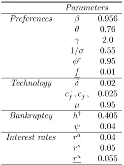
Parameters Preferences 0.956 0.76 2.0 1= 0.55 r _0.95 f 0.01 Technology 0.02 c+_f; c_f; 0.025 0.95 Bankruptcy hy _0.405 0.04 Interest rates ra _0.04 rs 0.05 ru _0.055

Table 2: Benchmark parameters for the calibrated numerical solution. Notes: The unit for

hy is the average of annual net labor earnings. Annualized parameters.

The adjustment costs are speci…ed symmetrically for upward and downward adjustments and are assumed to equal 2.5% of the stock, consistent with typical fees charged by real-estate brokers in the U.S. (Díaz and Luengo-Prado, 2010). These adjustment costs per se would imply that the consumer can use at most 97.5% of the housing stock to secure debt. Given the information of the Federal Deposit Insurance Corporation (FDIC) on real estate lending standards and supervisory loan-to-value limits, we calibrate access to secured consumer credit as slightly more restrictive with a loan-to-value ratio of 95%, = 0:95.17

The parameters for the bankruptcy procedure are set as follows. We set the value of the exempt home equity amounts equal to two …fths of average annual labor earnings which shall approximate the homestead exemption in the U.S. although there is signi…cant variation across U.S. states (Athreya, 2006). As we will discuss further below, the size of the exemption has little e¤ect on our results in strong contrast to Athreya (2006) or Pavan (2008) who do not analyze housing wealth, secured and unsecured debt jointly.

As in Livshits et al. (2007), we assume a small-open economy and set the annual risk-free lending rate to 4%. We assume a small transaction cost for debt so that the secured

17_{Information about supervisory loan-to-value limits is available at}

borrowing rate is 5% and the unsecured borrowing rate without the risk premiumru _{is 5.5%.} As we will see below, positive bankruptcy incidence in equilibrium implies an additional endogenous risk premium for unsecured debt. Allowing for interest spreads in the model is supported by empirical evidence in Davis, Kubler and Willen (2006), historical interest-rate data of the Federal Reserve (Table H.15) and is similar to assumptions in Athreya (2006) and Livshits et al. (2007).18

For the preference parameters, we setf= 0:01, a small and quantitatively negligible value, which allows consumers to consume no housing. We calibrate the remaining preference parameters , , , , r _{and to match the average statistics for the wealth and debt} portfolio and the home ownership rate for households up to the 90th percentile of the net worth distribution. The reason is that, as mentioned in Section 2.2, standard incomplete-market models cannot match the substantial wealth holdings in the top decile of the wealth distribution. Calibrating such a model to match average wealth in the whole sample would worsen the …t of the model for consumers up to the 90th percentile. These consumers would hold more wealth than observed the data, a prediction bias which is undesirable given that the focus of this paper is on debt portfolios.

Table 3 shows that for = 0:956, = 0:76,1= = 0:55, = 2, r _{= 0:95and = 0:04the} model matches the data targets well. The parameter values for patience, the weight of non-durable consumption in the consumption index, the intertemporal elasticity of substitution and risk aversion are within the range of commonly calibrated values. Rental e¢ ciency r₌

0:95helps to attain a realistic home ownership rate and the utility bankruptcy penalty = 0:04allows us to generate empirically observed unsecured debt holdings for renters. For = 0, unsecured debt would be prohibitively expensive for renters. Given that the preferences are homogeneous of degree 1, = 0:04can interpreted as a 4%smaller consumption basket. Concerning the incidence of bankruptcy reported in Table 3, we adjust the data target for bankruptcy reported in the SCF 2004 downward to 1.1% (1:67 2=3) since job-related shocks trigger bankruptcy in our model and two thirds of the bankruptcies are job related (Sullivan et al., 2000). The calibrated model predicts a smaller bankruptcy incidence of 0.4%, more similar to the data target for bankruptcy of 0.5% in Chatterjee et al. (2007).

SCF 2004 Model

Variable (1) (2)

Housing wealth (as fraction of net lab. earnings) 2.50 2.57 Net-…nancial assets (as fraction of net lab. earnings) -0.01 -0.01 Secured debt (as fraction of net lab. earnings) -0.75 -0.64 Unsecured debt (as fraction of net lab. earnings) -0.04 -0.03 Financial assets (as fraction of net lab. earnings) 0.77 0.66 Home ownership (% of sample) 64.4 66.7 Job-related bankruptcy (% of sample) 1.1 0.4

Table 3: Averages of the targets in the data and the model. Source: Authors’calculations based on the SCF and the model. Notes: *Bankruptcy incidence of 1.67 % in the data is multiplied by 2/3 for the fraction of job-related bankruptcies as reported in Sullivan et al. (2000). The unit is the average of net labor earnings.

This positive incidence of bankruptcy in equilibrium implies an average risk premium for unsecured debt of 2.1 percentage points. In addition to the results reported in Table 3, the model matches the incidence of debt rather well: 56% of consumers hold debt compared with 46% in the data, 46% hold secured debt compared with 39% in the data and 14% hold unsecured debt compared with 13% in the data. Finally, our model reproduces the empirical facts that consumers with unsecured debt are younger, have smaller labor earnings than the sample mean, own smaller but non-negligible amounts of housing wealth than the rest of the sample with substantial amounts of secured debt written against this collateral.

4.4

Life-cycle pro…les and cross-sectional age pro…les

After describing the calibration of the model and its ability to match our target statistics in the data, we now present the implications of our calibration for the cross-sectional age pro…les which are observed in the SCF. These pro…les have not been targeted explicitly by our calibration and thus give us a further indication of the model …t of the data. We …rst present the life-cyle pro…les of the model for the whole sample before computing the cross-sectional age pro…les for our sample of interest: prime-age consumers up to the 90th percentile of the net worth distribution.

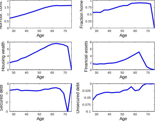
30 40 50 60 70 0 0.5 1 1.5 2 Age No n-d ur . co n s. 30 40 50 60 70 0 0.25 0.5 0.75 1 Age F raction h ome 30 40 50 60 70 0 2 4 6 8 Age H ousi ng w eal th 30 40 50 60 70 0 2 4 6 8 Age F in a nc ia l a ss et s 30 40 50 60 70 -3 -2 -1 0 Age S ec ured d ebt 30 40 50 60 70 -0.1 -0.075 -0.05 -0.025 0 Age U ns ec ured d ebt

Figure 3: Life-cycle pro…les predicted by the model. Source: Authors’calculations based on the model. Note: The unit is the average of net labor earnings.

of 100,000 consumers between ages 26 and 76.19 _{Non-durable consumption increases over}

the life cycle together with average earnings and housing wealth in our incomplete-markets life-cycle model. Financial assets display the familiar tent shape over the life cycle whereas housing wealth is hump-shaped. The home ownership rate steadily increases over the life-cycle before consumers sell their owned housing wealth at the end of life. Unsecured debt is largest (in absolute terms) for young consumers and then decreases with age.20 Secured debt …rst increases (in absolute terms) with age, then decreases before retirement, and increases again during the retirement period. As expected, consumers substantially reduce their home equity and …nancial assets during retirement. Home equity, that is housing wealth net of secured debt, drops by a large amount in the penultimate period when much of the …nancial assets have been depleted already.

These rather pronounced patterns towards the end of the retirement period clearly result from the assumption of a …nite life. In particular, the patterns of asset decumulation depend on the calibrated values for adjustment costs and rental e¢ ciency. Although the focus of this paper is not on explaining debt and wealth portfolios during retirement, we calibrate a more gradual reduction of home ownership in the retirement period to check that the model predictions for prime-age consumers are robust. Since this calibration requires di¤erent parameters for rental e¢ ciency or adjustment costs during retirement compared with the rest of life, we prefer our simpler calibration.

After presenting the life-cycle pro…les, we are now interested in how the cross-sectional age pro…les predicted by the model compare with the observed SCF cross-sections for our sample of interest. Figure 4 displays the average cross-sectional age pro…les for consumers between ages 26 and 55 up to the 90th percentile of the net worth distribution in the model (the solid graphs) and SCF data (the dashed graphs).21 _{In order to compare the life-cycle} 19_{At age 23 consumers start with a random draw from the SCF-data distribution of housing wealth and}

net-…nancial assets and a random draw for the income shock.

20_{The non-monotonic behavior of unsecured debt at age 60 is related to the last income shock before}

retirement which is “permanent”. The last shock determines retirement income (see the appendix on the calibration of the income process) and some consumers …nd it attractive to insure against this shock by holding unsecured debt which can be written o¤ if bankruptcy is declared. Indeed, we observe a spike in the bankruptcy incidence in the period of the last income shock (1% of consumers declare bankruptcy in the last period before retirement). The bankruptcy incidence then falls to zero during the retirement period when there is no more income uncertainty.

21_{Note that in the model, as for the average SCF statistics in Table 1, conditioning on consumers up to}

30 40 50 0 0.2 0.4 0.6 0.8 1 Age Fr act ion w ith home 30 40 50 0 0.5 1 1.5 2 2.5 3 3.5 Age H o usi ng w ealth 30 40 50 0 0.5 1 1.5 2 2.5 3 3.5 Age Financial as sets 30 40 50 -1 -0.8 -0.6 -0.4 -0.2 0 Age S ecure d deb t 30 40 50 -0.1 -0.08 -0.06 -0.04 -0.02 0 Age U nsec ur ed debt 30 40 50 0 0.01 0.02 0.03 0.04 0.05 Age Fr act ion bankrupt

Figure 4: Cross-sectional age pro…les predicted by the model (solid graph) and the data (dashed graph) for prime-age consumers with ages 26–55 up to the 90th percentile of the net worth distribution. Source: Authors’ calculations based on the model and the Survey of Consumer Finances (SCF) 2004. Notes: The unit is the average of net labor earnings. The bankruptcy incidence in the data is multiplied by 2/3 for the fraction of job-related bankruptcies as reported in Sullivan et al. (2000). See the data appendix for variable de…nitions.

model output with the SCFcross-section data, we have adjusted the simulation output of the model accounting for cohort e¤ects resulting from income growth (see Section 4.2). Figure 4 shows that the cross-sectional age pro…les predicted by the model match the SCF data pro…les remarkably well: home ownership rates, owner-occupied housing wealth and …nancial assets increase between ages 26 and 55, whereas secured and unsecured debt decrease between ages 26 and 55 in absolute terms. Noting the di¤erent scale for secured and unsecured in Figure 4, the model predicts that debt is mostly secured as in the data. Moreover, we …nd that about a third of young consumers with housing wealth at the beginning of life is at the collateral constraint. For the relevant parameters which produce a quantitative …t of the facts, consumers close to, or at, the collateral constraint with little housing equity hold the more expensive unsecured debt. Most consumers repay their unsecured debt and the bankruptcy incidence falls between ages 26 and 55 both in the model and the data. The model predicts somewhat more bankruptcies for young consumers than the SCF data which may not be of major concern, however, given that the cross-sectional age pro…le for bankruptcy is quite noisily measured in the data.

4.5

Sensitivity analysis

Given the good …t of the model with the SCF data, we perform three experiments in order to better understand the model. We compute special cases of the model in which consumers do not have access to secured debt, unsecured debt and the bankruptcy option, respectively. This will help to understand the importance of the debt instruments and the bankruptcy option in the model for intratemporal and intertemporal consumption smoothing. Moreover, the experiments provide intuition for the role of home equity as informal collateral which is of major interest in this paper.

Preferences in our model imply consumption smoothing across states and across time. We compute the variance of the logarithm of the consumption basket (including rented or owned housing wealth) as an indicator for intratemporal consumption smoothing and average total debt (the sum of secured and unsecured debt) as an indicator for the extent of intertemporal consumption smoothing. Figure 5 displays the results for these indicators for the benchmark calibration and our experiments.

30 40 50 0 0.1 0.2 0.3 0.4 0.5 0.6 0.7 0.8 0.9 1 Age V ar iance of log(cons.bas ket) Benchmark No secured No unsecured No bankrupt 30 40 50 -1.5 -1.25 -1 -0.75 -0.5 -0.25 0 Age D ebt Benchmark No secured No unsecured No bankrupt 30 40 50 0 0.5 1 1.5 2 2.5 3 3.5 Age H ome equity Benchmark No secured No unsecured No bankrupt

Figure 5: The variance of the log consumption basket, average debt and home equity for the benchmark and three experiments. Source: Authors’calculations based on the model. Notes: The unit is the average of net labor earnings. Debt is the sum of secured and unsecured debt. Home equity is housing wealth net of secured debt.

In our benchmark calibration the variance of the log consumption basket, plotted as the solid graph, has a concave shape for consumers between ages 26 and 55, as in the model without housing and secured debt in Livshits et al. (2007), Figure 3B. If agents do not have access to unsecured debt, the variance of the log consumption basket, plotted as the dash-dotted graph, increases by up to 0.1 for young consumers compared with the benchmark calibration. This is a sizeable increase of the variance by 25%. After age 40, the variance is very similar to the benchmark. As illustrated in the graph for total debt, young consumers take on less total debt (in absolute terms) to smooth consumption if they do not have access to unsecured debt and can only borrow against housing collateral. Unsecured debt is thus important for young consumers to smooth consumption across states and time.

If the consumer has no bankruptcy option, total debt (plotted as the dotted graph in Figure 5) increases substantially in absolute terms due to an increase in unsecured debt.22

We …nd that full repayment commitment reduces the risk premium on unsecured debt and thus allows consumers to smooth consumption more cheaply intertemporally. The e¤ect on intratemporal consumption smoothing is unclear, however, since bankruptcy allows to smooth consumption after the realization of bad income states. We …nd that the variance of the log consumption basket decreases for young consumers and increases after age 40 com-pared with the benchmark case, similar to results reported in Livshits et al. (2007), Figure 3B. Interestingly, Figure 5 also shows that home equity decreases if there is no bankruptcy option and thus full repayment commitment: both housing wealth and secured debt decrease in absolute terms but housing wealth decreases more strongly. At …rst glance, one might be tempted to read this …nding as pointing to a potential role of home equity as informal collat-eral. The next section demonstrates, however, that home equity does not provide informal collateral in our quantitative model.

If the consumer has no access to secured debt, average owned housing wealth falls nearly by the same amount so that average home equity is very close to the benchmark case. In Figure 5 this is illustrated by the dashed and the solid graph. Since the home ownership rate falls from 67% to 39%, this home equity is held by a much smaller fraction of consumers so

22_{The case with no bankruptcy option is implemented by setting = 1. This implies that the value is zero}

if bankruptcy is declared, which is strictly smaller than the strictly positive value under repayment. Thus, the max-operator in equations (7) and (9) is redundant and the problem is equivalent to a problem without a bankruptcy option.

that the home equity per owner is larger if there is no access to secured debt. Lack of access to secured debt implies that housing wealth equals home equity. This makes bankruptcy less attractive for owners who have …nanced their housing purchase with debt, since home equity is much larger than the exempt level in bankruptcy procedures for most owners. Indeed, consumers no longer declare bankruptcy in equilibrium in the model case without secured debt. Although all debt is unsecured debt in this case, banks are willing to lend unsecured debt so that average total debt is very similar to the benchmark case. Moreover, the age pro…le of the variance of the log-consumption basket is qualitatively similar to the case without a bankruptcy option, where the variance in the case without secured debt is quantitatively larger after age 40. In Figure 5 this illustrated by the dashed and the dotted graph.

5

Commitment by home equity?

Compared with the existing literature a new feature of our model is the joint analysis of housing wealth, secured and unsecured debt since we do not fully consolidate the household balance sheet by computing a single measure of net worth. As we will see, the joint analysis a¤ords new insights for the quantitative importance of committing by using home equity as informal collateral.

Home equity provides informal collateral for unsecured debt if home equity, net of adjust-ment cost, is above the exemption level hy _{= 0:405. In this case unsecured creditors receive}

some repayment since the bankruptcy judge will sell housing wealth in order to repay some of the unsecured debt. Thus, home equity above the exemption level hy _{makes bankruptcy}

less attractive for consumers, also because of the wasteful adjustment costs, and allows them cheaper access to unsecured debt since banks realize that home equity above the exemption level hy _{provides informal collateral.}

To gauge the quantitative importance of home equity as informal collateral in our model, Figure 6 plots the price for unsecured debt in our benchmark calibration as a function of unsecured debt for di¤erent values of housing wealth. As an example, we plot graphs for young consumers at ages 26–28 in the fourth income state. Since consumers who hold

-3 -2 -1 0 0 0.1 0.2 0.3 0.4 0.5 0.6 0.7 0.8 0.9 Unsecured debt Pr ic e (pe r annu m) Housing wealth = 0 -30 -2 -1 0 0.1 0.2 0.3 0.4 0.5 0.6 0.7 0.8 0.9 Unsecured debt Pr ic e (pe r annu m) Housing wealth = 1.7 -3 -2 -1 0 0 0.1 0.2 0.3 0.4 0.5 0.6 0.7 0.8 0.9 Unsecured debt Pr ic e (pe r annu m) Housing wealth = 5 -30 -2 -1 0 0.1 0.2 0.3 0.4 0.5 0.6 0.7 0.8 0.9 Unsecured debt Pr ic e (pe r annu m) Housing wealth = 8.1

Figure 6: The price of unsecured debt as a function of unsecured debt for di¤erent housing wealth. Source: Authors’calculations based on the model. Notes: Prices are per annum for consumers who are at the collateral constraint in the fourth income state at ages 26–28. The unit of unsecured debt is the average of annual net labor earnings.