䊚
A Prefix Code Matching Parallel Load-Balancing
Method for Solution-Adaptive Unstructured
Finite Element Graphs on Distributed
Memory Multicomputers
YEH-CHING CHUNG, CHING-JUNG LIAO,
DON-LIN YANG ychung, cjliao, [email protected]
Department of Information Engineering, Feng Chia Uni¨ersity, Taichung, Taiwan 407, ROC ŽRecei¨ed February 18, 1998; final¨ersion accepted No¨ember 13, 1998..
Ž .
Abstract. In this paper, we propose a prefix code matching parallel load-balancing method PCMPLB to efficiently deal with the load imbalance of solution-adaptive finite element application programs on distributed memory multicomputers. The main idea of the PCMPLB method is first to construct a prefix code tree for processors. Based on the prefix code tree, a schedule for performing load transfer among processors can be determined by concurrently and recursively dividing the tree into two subtrees and finding a maximum matching for processors in the two subtrees until the leaves of the prefix code tree are reached. We have implemented the PCMPLB method on an SP2 parallel machine and compared its performance with two load-balancing methods, the directed diffusion method and the multilevel diffusion method, and five mapping methods, the AErORB method, the AErMC method, the MLkP method, the PARTY library method, and the JOSTLE-MS method. An unstructured finite element graph Truss was used as a test sample. During the execution, Truss was refined five times. Three criteria, the execution time of mappingrload-balancing methods, the execution time of an application program under different mappingrload-balancing methods, and the speedups achieved by mappingr load-balancing methods for an application program, are used for the performance evaluation. The
Ž .
experimental results show that 1 if a mapping method is used for the initial partitioning and this mapping method or a load-balancing method is used in each refinement, the execution time of an
Ž .
application program under a load-balancing method is less than that of the mapping method. 2 The execution time of an application program under the PCMPLB method is less than that of the directed diffusion method and the multilevel diffusion method.
Keywords: distributed memory multicomputers, partitioning, mapping, remapping, load balancing, solution-adaptive unstructured finite element models
1. Introduction
The finite element method is widely used for the structural modeling of physical
w x
systems 27 . To solve a problem using the finite element method, in general, we need to establish the finite element graph of the problem. A finite element graph is a connected and undirected graph that consists of a number of finite elements. Each finite element is composed of a number of nodes. The number of nodes of a finite element is determined by an application. In Figure 1, an example of a 21-node finite element graph consisting of 24 finite elements is shown. Due to the
Ž
Figure 1. An example of a 21-node finite element graph with 24 finite elements the circled and
.
uncircled numbers denote the node numbers and finite element numbers, respectively .
properties of computation-intensiveness and computation-locality, it is very attrac-tive to implement the finite element method on distributed memory
multicomput-w x
ers 1, 41᎐42, 47᎐48 . In the context of parallelizing a finite element application
w x
program that uses iterative techniques to solve a system of equations 2᎐3 , a parallel program may be viewed as a collection of tasks represented by nodes of a finite element graph. Each node represents a particular amount of computation and can be executed independently.
To efficiently execute a finite element application program on a distributed memory multicomputer, we need to map nodes of the corresponding graph to processors of the multicomputer such that each processor has approximately the same amount of computational load and the communication among processors is
w x
minimized. Since this mapping problem is known to be NP-complete 13 , many
w
heuristic methods were proposed to find satisfactory suboptimal solutions 4᎐6, 8,
x
10᎐11, 14᎐15, 17᎐18, 24᎐26, 29, 31, 33, 35, 41, 43᎐44, 47᎐48 .
If the number of nodes of a finite element graph does not increase during the execution of a finite element application program, the mapping algorithm only needs to be performed once. For a solution-adaptive finite element application program, the number of nodes increases discretely due to the refinement of some finite elements during the execution. This may result in load imbalance of proces-sors. A node remapping or a load-balancing algorithm has to be performed many times in order to balance the computational load of processors while keeping the communication cost among processors as low as possible. For the node remapping approach, some mapping algorithms can be used to partition a finite element graph from scratch. For the load-balancing approach, some load-balancing algorithms can be used to perform the load balancing process according to the current load of processors. Since node remapping or load-balancing algorithms are performed at run-time, their execution must be fast and efficient.
In this paper, we propose a prefix code matching parallel load-balancing
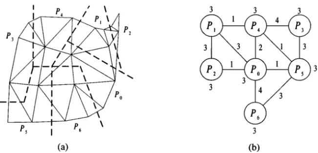
ŽPCMPLB method to efficiently deal with the load imbalance of solution-adaptive. finite element application programs on distributed memory multicomputers. In a finite element graph, the value of a node depends on the values of node and other nodes that are in the same finite elements of node. For example, in Figure 1, nodes 3, 5, and 6 form element 3, nodes 5, 6, and 9 form element 5, and nodes 6, 9, and 10 form element 8. The value of node 6 depends on the values of node 6, node 3, node 5, node 9, and node 10. When nodes of a solution-adaptive finite element graph were evenly distributed to processors by some mapping algorithms, two processors, Pi and Pj, need to communicate to each other if two nodes in the same finite element are mapped to Pi and Pj, respectively. According to this communication property of a partitioned finite element graph, we can get a processor graph from the mapping. In a processor graph, nodes represent the processors and edges represent the communication needed among processors. The weights associated with nodes and edges denote the computation and the
commu-Ž .
nication costs, respectively. Figure 2 a shows a mapping of Figure 1 on 7
proces-Ž . Ž .
sors. The corresponding processor graph of Figure 2 a is shown in Figure 2 b . When a finite element graph is refined at run-time, it may result in load imbalance of processors. To balance the computational load of processors, the PCMPLB method is first to construct a prefix code tree for processors according to the processor graph, where the leaves of the prefix code tree are processors. Based on the prefix code tree, a schedule for performing load transfer among processors can be determined by concurrently and recursively dividing the tree into two subtrees and finding a maximum matching for processors in the two subtrees until the leaves of the prefix code tree are reached.
We have implemented this method on an SP2 parallel machine and compared its
w
performance with two load-balancing methods, the directed diffusion method 9,
x w x
44 and the multilevel diffusion method 37᎐38 , and five mapping methods, the
Ž . Ž .
Figure 2. a A mapping of Figure 1 on 7 processors. b The corresponding processor graph of
Fig-Ž .
w x w x
AErORB method 4, 8, 29, 48 , the AErMC method 8, 10, 12, 14, 26 , the MLkP
w x w x
method 24 , the PARTY library method 35 , and the JOSTLE-MS method
w43᎐46 . An unstructured finite element graphx Truss was used as the test sample. During the execution, Truss was refined five times. Three criteria, the execution time of mappingrload-balancing methods, the execution time of an application program under different mappingrload-balancing methods, and the speedups achieved by mappingrload-balancing methods for an application program, are used
Ž . for the performance evaluation. The experimental results show that 1 if a mapping method is used for the initial partitioning and this mapping method or a load-balancing method is used in each refinement, the execution time of an application program under a load-balancing method is less than that of the
Ž .
mapping method. 2 The execution time of an application program under the PCMPLB method is less than that of the directed diffusion method and the multilevel diffusion method.
The paper is organized as follows. The related work is given in Section 2. In Section 3, the proposed prefix code matching parallel load-balancing method is described in detail. In Section 4, we present the cost model of mappingr load-bal-ancing methods for unstructured finite element graphs on distributed memory multicomputers. The performance evaluation and simulation results are also pre-sented in this section.
2. Related work
Many methods have been proposed to deal with the load unbalancing problems of solution-adaptive finite element graphs on distributed memory multicomputers in the literature. They can be classified into two categories, the remapping method and the load redistribution method. For the remapping method, many finite element graph mapping methods can be used as remapping methods. In general,
w x
they can be divided into five classes, the orthogonal sectionapproach 4, 8, 29, 48 ,
w x w x
the min-cut approach 8, 10, 12, 14, 26 , the spectral approach 5᎐6, 41 , the
w x w x
multile¨el approach 5᎐6, 19, 24᎐25 , and others 15, 31, 34, 41 . These methods
w x
were implemented in several graph partition libraries, such as Chaco 17 , DIME
w x48 , JOSTLE 45 , METIS 24w x w ᎐25 , PARTY 35 , Scotch 33 , and TOPx w x w x rDOMDEC
w x11 , etc., to solve graph partition problems. Since our main focus is on the load-balancing methods, we do not describe these mapping methods here.
For the load redistribution method, many load-balancing algorithms can be used
w x
as load redistribution methods. In 46 , a recent comparison study of dynamic load balancing strategies on highly parallel computers is given. The dimension exchange
Ž . w x
method DEM is applied to application programs without geometric structure 9 . It is conceptually designed for a hypercube system but may be applied to other
w x w x
topologies, such as k-ary n-cubes 51 . Ou and Ranka 32 proposed a linear programming-based method to solve the incremental graph partition problem. Wu
w39, 49 proposed the tree walking, the cube walking, and the mesh walking runx
time scheduling algorithms to balance the load of processors on tree-base, cube-base, and mesh-base paradigms, respectively.
w x
Hu and Blake 22 proposed a directed diffusion method that computes the diffusion solution by using an unsteady heat conduction equation while optimally minimizing the Euclidean norm of the data movement. They proved that the diffusion solution could be found by solving the linear equation. The diffusion solution is a vector with nelements. For any two elements i,j in , if iyj
is positive, then partition i needs to send iyj nodes to partition j. Otherwise,
w x
partition j needs to send jyi nodes to partition i. Heirich and Taylor 16 proposed a direct diffusive load balancing method for scalable multicomputers. They derived a reliable and scalable load balancing method based on properties of the parabolic heat equation u y␣ⵜ2us0.
t w x
Horton 20 proposed a multilevel diffusion method by recursively bisecting a communication graph into two subgraphs and balancing the load of processors in the two subgraphs. In each bisection, the two subgraphs are connected by one or more edges and the difference of processors in the two subgraphs is less than or equal to 1.
w x
Schloegel et al. 38 also proposed a multilevel diffusion scheme to construct a new partition of the graph incrementally. It contains three phases, a coarsening phase, a multilevel diffusion phase, and a multilevel refinement phase. A parallel
w x
multilevel diffusion algorithm was also described in 37 . These algorithms perform diffusion in a multilevel framework and minimize data movement without compris-ing the edge-cut. Their methods also include parameterized heuristics to specifi-cally optimize edge-cut, total data migration, and the maximum amount of data migrated in and out of any processor.
w x
Walshaw et al. 44 implemented a parallel partitioner and a directed diffusion
w x
repartitioner in JOSTLE 45 . The directed diffusion method is based on the
w x
diffusion solver proposed in 22 . It has two distinct phases, the load-balancing phase and the local refinement phase. In the load-balancing phase, the diffusion solution guides vertex migration to balance the load of processors. In the local refinement phase, a local view of the graph guides vertex migration to decrease the number of cut-edges between processors. They also developed a multilevel diffu-sion repartitioner in JOSTLE.
w x
Oliker and Biswas 30 presented a novel method to dynamically balance the processor workloads with a global view. Several novel features of their framework were described such as the dual graph repartition, the parallel mesh repartitioner, the optimal and heuristic remapping cost functions, the efficient data movement and refinement schemes, and the accurate metrics comparing the computational gain and the redistribution cost. They also developed generic metrics to model the remapping cost for multiprocessor systems.
3. The prefix code matching parallel load-balancing method
To deal with the load imbalance of a solution-adaptive finite element application program on a distributed memory multicomputer, a load-balancing algorithm needs to balance the load of processors and minimize the communication among proces-sors. Since a load-balancing algorithm is performed at run-time, the execution of a load-balancing algorithm must be fast and efficient. In this section, we will describe
a fast and efficient load-balancing method, the prefix code matching parallel
Ž .
load-balancing PCMPLB method, for solution-adaptive finite element application programs on distributed memory multicomputers in detail.
The main idea of the PCMPLB method is first to construct a prefix code tree for processors. Based on the prefix code tree, a schedule for performing load transfer among processors can be determined by concurrently and recursively dividing the tree into two subtrees and finding a maximum matching for processors in the two subtrees until the leaves of the prefix code tree are reached. Once a schedule is determined, a physical load transfer procedure can be carried out to minimize the communication overheads among processors. The PCMPLB method can be divided into the following four phases.
Phase 1: Obtain a processor graph G from the initial partition. Phase 2: Construct a prefix code tree for processors in G.
Phase 3: Determine the load transfer sequence by using matching theorem. Phase 4: Perform the load transfer.
In the following, we will describe them in detail.
3.1. The processor graph
In a finite element graph, the value of a node depends on the values of node and other nodes that are in the same finite elements of node . When nodes of a solution-adaptive finite element graph were distributed to processors by some mapping algorithms, two processors, Piand Pj, need to communicate to each other if two nodes in the same finite element are mapped to Pi and Pj, respectively. According to this communication property of a partitioned finite element graph, we can get a processor graph from the mapping. In a processor graph, nodes represent the processors and edges represent the communication needed among processors. The weights associated with nodes and edges denote the computation and the communication costs, respectively. We now give an example to explain it.
Ž .
Example 1. Figure 3 shows an example of a processor graph. Figure 3 a shows an initial partition of a 100-node finite element graph on 10 processors by using the
Ž .
MLkP method. In Figure 3 a , all processors are assigned 10 finite element nodes. After a refinement, the number of nodes assigned to processors P0,P1,P2,P3,P4,
P5,P6,P7,P8, and P9 are 10, 11, 11, 12, 10, 19, 16, 13, 13, and 13, respectively, and
Ž . Ž .
is shown in Figure 3 b . The corresponding processor graph of Figure 3 b is shown Ž .
in Figure 3 c .
3.2. The construction of a prefix code tree
Based on the processor graph, we can construct a prefix code tree. The algorithm
w x
for construction of a prefix code tree TP r e f i x is based on Huffman’s algorithm 23 and is given as follows.
Ž . Ž . Figure 3. An example of a processor graph. a The initial partitioned finite element graph. b The
Ž . Ž .
finite element graph after a refinement. c The corresponding processor graph obtained from b .
Ž .
Algorithm build prefix code tree G᎐ ᎐ ᎐
1 LetV be a set of P isolated vertices, where P is the number of processors in a processor graph G. Each vertex Pi in V is the root of a complete
Ž .
binary tree of height 0 with a weight wis1.
< <
2 While V )1
3
4 Find a tree T in V with the smallest root weight w. If there are two or more candidates, choose the one whose leaf nodes have the smallest degree in G.
5 For trees in V whose leaf nodes are adjacent to those in T, find a tree
T⬘with the smallest root weight w⬘. If there are two or more candidates, choose the one whose leaf nodes have the smallest degree in G.
Ž .
6 Create a new complete binary tree T* with root weight w*swqw⬘
and having T and T⬘as its left and right subtrees, respectively. 7 Place T* in V and deleteT and T⬘.
4 8
end of build prefix code tree᎐ ᎐ ᎐ ᎐ ᎐
We now give an example to explain algorithm build prefix code tree᎐ ᎐ ᎐ .
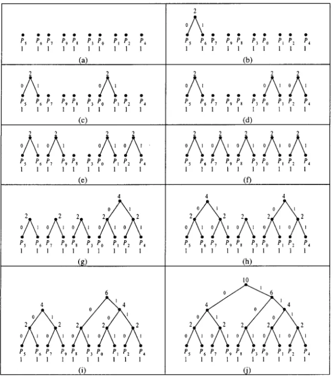
Example 2. An example of step by step construction of a prefix code Ž .
tree from the processor graph shown in Figure 3 c is given in Figure 4. The degrees of processors P0,P1,P2,P3,P4,P5,P6,P7,P8, and P9 are 3, 3, 3, 6, 4, 2, 4, 4, 4, and 5, respectively. The initial configuration is shown
Ž .
in Figure 4 a . In the first iteration of lines 2᎐8 of algorithm build pre᎐
-fix code tree᎐ ᎐ , P5 has the smallest degree among those trees with root weights1. P5 is selected as the candidate in line 4. In line 5, both P6
and P7 are adjacent to P5 with root weights1. The degrees of P6 and
P7 are the same. We choose P6 as the candidate because P6 has a smaller rank. P5 and P6 are then combined as a tree in line 6. After the execution of line 7, we obtain a new configuration as shown in Figure
Ž .
Ž . Figure 4. A step by step construction of a prefix code tree from Figure 3 c .
line 5. After the execution of lines 6 and 7, we obtain a new configura-Ž .
tion as shown in Figure 4 c . By continuing the iteration seven times, we Ž . Ž .
can obtain Figures 4 d ᎐4 j .
3.3. Determine a load transfer sequence by using matching theorem
Based on the prefix code tree and the processor graph, we can obtain a communi-cation pattern graph.
Ž .
Definition 1. Given a processor graph Gs V,E and a prefix code tree TP r e f i x,
Ž .
the communication pattern graph Gcs Vc,Ec of G andTP r e f i x is a subgraph of
Ž .
G. For every Pi,Pj gEc,Pi and Pj are in the left and the right subtrees of
TP r e f i x, respectively, and Pi,PjgVc.
The communication pattern graph has several properties that can be used to determine the load transfer sequence.
Ž .
Definition 2. A graph Gs V,E is called bipartiteif VsV1jV2 withV1lV2
Ž .
s, and every edge of G is of the form a,b with agV1 and bgV2.
Theorem 1. A communication pattern graph G is a bipartite graphc .
Ž .
Proof: According to Definition 1, for every Pi,Pj gEc,Pi and Pj are in the left and right subtrees of TP r e f i x, respectively. ThereforeGc is a bipartite graph. I
Definition 3. A subset M of Eis called a matching inG if its elements are edges and no two of them are adjacent in G; the two ends of an edge in Mare said to be matched under M. M is a maximum matching if G has no matching M⬘ with
<M⬘<)< <M.
Ž . Ž .
Theorem 2. Let Gs V,E be a bipartite graph with bipartition V1,V2 .Then G
< Ž .< < <
contains a matching that saturates e¨ery¨ertex in V if and only if N S1 G S for all
Ž .
S:V1,where N S is the set of all neighbors of¨ertices in S.
w x
Proof: The proof can be found in 7 . I
Ž .
Corollary 1. Let Gcs Vc,Ec be a communication pattern graph and V and VL R are the sets of processors in the left and the right subtrees of TP r e f i x,respeci¨ely,where VL,VR:Vc.Then we can find a maximum matching M from G such that for ec ¨ery
Ž .
element Pi,Pj gM,PigV and PL jgVR.
w x
Proof: From Theorem 2 and Hungarian method 7 , we know that a maximum
matching M fromGc can be found. I
From the communication pattern graph, we can determine a load transfer sequence for processors in the left and the right subtrees of a prefix code tree by using the matching theorem to find a maximum matching among the edges of the communication pattern graph. Due to the construction process used in Phase 2, we can also obtain communication pattern graphs from the left and the right subtrees of a prefix code tree. A load transfer sequence can be determined by concurrently and recursively performing the following steps,
Step 1. Divide a prefix code tree into two subtrees,
Step 3. Find a maximum matching for the communication pattern graph, and Step 4. Determine the number of finite element nodes to be transferred among
processors,
until a tree contains only one vertex.
Assume that a processor graph has P processors and a refined finite element graph has N nodes. We define NrP as the average load of a processor. The load of a processor is defined as the number of finite element nodes assigned to it. Let
Ž . Ž .
load Pi and quota Pi represent the load and the average load of processor Pi, respectively. The algorithm to determine a load transfer sequence is given as follows.
Ž .
Algorithm determine load transfer sequence G᎐ ᎐ ᎐ ,TP r e f i x
1 Let ST be a set that contains the prefix code tree obtained in Phase 2 and
seqs0;
< <
2 while ST -P r*P is the number of processors in G*r
Ž .
3 ᭙TP r e f i xgST,if the number of vertices inTP r e f i x)1 then
4 Let TL and TR be the left and the right subtrees of TP r e f i x, respec-tively;
5 Find the communication pattern graph Gc from the processor graphG
and the prefix code treeTP r e f i x;
Ž .<
6 Find a maximum matching Ms Pi,Qi Pi and Qi are processors in 4
TL and TR, respectively, and Pi and Qi are adjacent in G from Gc; Ž .
7 quota TR sthe sum of the average load of processors in TR; Ž .
8 load TR sthe sum of the load of processors inTR;
Ž Ž . Ž ..
9 if load TR )quota TR then
10 seqsseqq1; LSs e qs⭋; Ž . 11 For each Pi,Qi in M,do Ž Ž . Ž .. < < 12 ms load TR yquota TR rM; Ž Ž . .
13 if load Pi -m then flags0else flags1;
Ž .4
14 LSs e qsLSs e qj Pi,Qi,m,flag ;
Ž . Ž . Ž . Ž .
15 load Pi sload Pi ym; and load Qi sload Qi qm; 4
16 4 17
Ž Ž . Ž .
18 else if load TR -quota TR then
19 seqsseqq1; LSs e qs⭋; Ž . 20 For each Pi,Qi in M,do Ž Ž . Ž .. < < 21 ms quota TR yload TR rM; Ž Ž . .
22 if load Qi -m then flags0else flags1;
Ž .4
23 LSs e qsLSs e qj Qi,Pi,m,flag ;
Ž . Ž . Ž . Ž .
24 load Pi sload Pi qm; and load Qi sload Qi ym; 4
25 4 26
27 PlaceTL andTR in ST and deleteTP r e f i x from ST; 4
28 4 29
r* Exception Handling *r
Ž Ž . .
30if ᭚ SP,RP,m, 0 gLSi, where is1, . . . ,seq then
Ž .
31 For each processor Pi, reset load Pi to its initial value;
Ž .
32 for ks1;kFseq;kq q
Ž .
33 For each element SP,RP,m,flag in LSk,do
Ž Ž . .
34 if load SP -m then flags0else flags1;
Ž . Ž . Ž . Ž . Ž .
35 if flags1 then load SP sload SP ym;load RP sload RP
4
qm
36 else
ŽŽ .
37 if SP,RP,m,flag can be performed with other elements in
. Ž .4
38 LSs e q in parallel then LSs e qsLSs e qj SP,RP,m,flag
Ž .4 4
39 else seqq q; LSs e qs SP,RP,m,flag ;
Ž .4 40 LSksLSky SP,RP,m,flag ; 4 41 4 42 4 43 4 44
end of determine load transfer sequence᎐ ᎐ ᎐ ᎐ ᎐
In the above description, lines 2᎐29 construct a load transfer sequence,
LS1,LS2, . . . ,LSs e q, according to the processor graph, the prefix code tree, and the matching theorem. Each step LSi in a load transfer sequence may contain more than one element. It means that the load transfer process for each processor pair in LSi can be performed in parallel. Lines 30᎐44 form an exception handling
Ž . Ž .
process. For an element SP,RP,m,flag in LSi, it is possible that load SP -m. In this case, if we perform the load transfer process, processor SP fails to send the desired nodes to processor RP. To avoid this situation, in the exception handling
Ž .
process, we postpone the execution of all elements SP,RP,m, 0 in LSi by moving them to the end of the sequence. We have the following theorem.
Theorem 3. By executing the load transfer sequence obtained from algorithm deter
-mine load transfer sequence᎐ ᎐ ᎐ , the load of processors can be fully balanced.
Proof: Assume that a processor graph has P processors and a refined finite element graph has N nodes, where N is divisible by P. According to lines 2᎐29, we know that a load transfer sequence, LS1,LS2, . . . ,LSs e q, can be generated. Each
Ž .
LSi is generated by lines 9᎐26, where is1, . . . ,seq. For a processor SP RP in ŽSP,RP,m,flag. of LS1,LS2, . . . ,LSs e q, it needs to send receiveŽ . m finite
ele-Ž . Ž .
ment nodes to from processorRP SP . Due to the method used to determine the load transfer numbers in lines 9᎐26, after a sequence of send and receive operations, the number of nodes in each processor will be equal to NrP. We have the following two cases.
Ž .
Case 1. If the value of flag of each element SP,RP,m,flag in LS1,LS2, , . . .LSs e q is equal to 1; that is, the load ofSP is always greater than or equal tom,
then the load of processors can be balanced after executing the load transfer sequence produced by lines 2᎐29. In this case, the load transfer sequence is obtained according to the communication pattern graphs and the maximum
match-u v
ing. The value of seq is equal to logP .
Ž .
Case 2. If there exists some elements SP,RP,m, 0 in LS1,LS2, . . . ,LSs e q, then a new load transfer sequence, LSX1,LSX2, . . . ,LSXs e q, is produced by lines 30᎐44. Since lines 30᎐44 only alter the execution order of elements in LS1,LS2, . . . ,LSs e q, the load transfer pairs and the number of finite element nodes needed to be transferred between processors in the load transfer pair in LSX1, . . . ,LSXs e q, are the same as those in LS1, . . . ,LSs e q. Therefore, if we can claim that the value of flag
Ž . X X X
of each element SP,RP,m,flag in LS1,LS2, . . . ,LSs e q, is equal to 1, then the load of processors can be balanced after the load transfer sequence
LS1X,LSX2, . . . ,LSXs e q, is performed.
Ž .
Let CGs V,E be a communication graph, where V is the set of processors
Ž .
that appear in the first two positions of elements SP, RP,m, flag in
LS1X,LSX2, . . . ,LSXs e q⬘, and E is the set of arcs that represent the sendrreceive
Ž . X X X
relations of SP and RP for elements SP,RP,m,flag in LS1,LS2, . . . ,LSs e q⬘. Obviously, CG is a digraph. Assume that there exists some elements ŽSP,RP,m,flag.in LS1X,LSX2, . . . ,LSXs e q⬘ in which the values of flag are equal to 0. According to lines 30᎐44, these elements are in LSXk, . . . ,LSXs e q⬘, where k)1. When we perform load transfer according to LSX1,LSX2, . . . ,LSXs e q⬘, whenever a processor sends nodes to another processor, we remove the corresponding sendrreceive relation from CG. After steps LSX1, . . . ,LSXky1 are performed, we have a communication graph CG⬘ that corresponds to the sendrreceive relations
Ž . X X
of elements SP,RP,m,flag in LSk, . . . ,LSs e q⬘. Since the value of flag for each
Ž . X X
element SP,RP,m,flag in LSk, . . . ,LSs e q⬘ is equal to 0, each processor in CG⬘
needs to receive nodes from other processors of CG⬘in order to balance its load. Therefore, the in-degree of each vertex in CG⬘ is greater than or equal to 1. It implies that CG⬘ contains loops. However, the construction of a load transfer sequence in lines 2᎐29 is based on the bipartite graphs and the maximum matching. CG contains no loops. Since CG⬘ is a subgraph of CG, it implies that
CG⬘ contains no loops either. This contradicts our assumption. Therefore, the
Ž . X X X
value of flag for each element SP,RP,m,flag in LS1,LS2, . . . ,LSs e q⬘ is equal to 1. In this case, the load transfer sequence is obtained according to lines 2᎐29 and
Ž .
lines 30᎐44. The number of elements SP,RP,m,flag that can be generated in
u v u v
lines 2᎐29 is less than or equal to logP = Pr2 . Therefore, the number of steps of the load transfer sequence generated by lines 30᎐44 is less than or equal to
ulogPv=uPr2 , i.e.,v seq⬘FulogPv=uPr2 .v I
We now give an example to explain the behavior of algorithm determine᎐ load transfer sequence᎐ ᎐ .
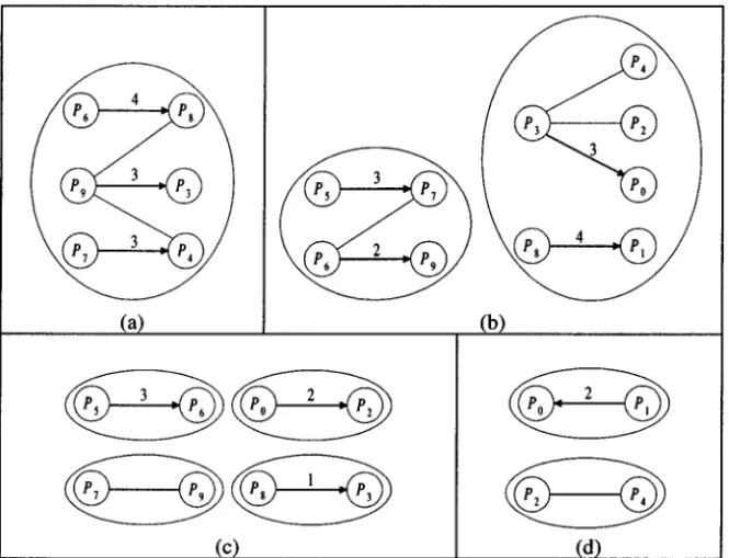
Example 3. Figure 5 shows the communication pattern graphs and the corre-sponding maximum matching for the example shown in Figures 3 and 4 step by step
Ž . when performing algorithm determine load transfer sequence᎐ ᎐ ᎐ . Figure 5 a shows the communication pattern graph for the prefix code tree with root at level 1. In
Ž . Ž .
Figure 5. The matching of the communication pattern graph. a The first matching. b The second
Ž . Ž .
matching. c The third matching. d The fourth matching.
Ž .
Figure 5 a , an arrow is an element of a matching. The number associated with an arrow denotes the number of finite element nodes that a processor needs to send
4
to another processor. In this case, TLs P5,P6,P7,P9,TRs P0,P1,P2,P3,
4 Ž . Ž . Ž . Ž .
P4,P8 ,load TL s61,load TR s67,quota TL s51, and quota TR s77. Ac-cording to line 20 of algorithm determine load transfer sequence᎐ ᎐ ᎐ , the processors in
TR need to receive 10 nodes from the processors in TL. From the communication
Ž . Ž .
pattern graph and the matching theorem, we have LS1s P6,P8, 4, 1 , P7,P4, 3, 1 , ŽP9,P3, 3, 1 . Figure 5 b to Figure 5 d show the communication pattern graphs.4 Ž . Ž . and the corresponding maximum matching for the prefix code trees with roots at levels 2, 3, and 4, respectively. After the execution of lines 2᎐29 of algorithm
determine load transfer sequence᎐ ᎐ ᎐ , we have the following load transfer sequence.
Ž . Ž . Ž .4 LS1s P6,P8, 4, 1 , P9,P3, 3, 1 , P7,P4, 3, 1 ; Ž . Ž . Ž . Ž .4 LS2s P5,P7, 3, 1 , P6,P9, 2, 1 , P3,P0, 3, 1 , P8,P1, 4, 1 ; Ž . Ž . Ž .4 LS3s P5,P6, 3, 1 , P0,P2, 2, 1 , P8,P3, 1, 1 ; Ž .4 LS4s P1,P0, 2, 1 . Ž .
Since the value of flag of each element SP,RP,m,flag in LS1, . . . ,LS4 is equal to 1, the execution of algorithm determine load transfer sequence᎐ ᎐ ᎐ is terminated.
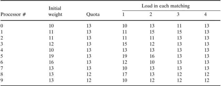
Table 1. The load of each processor in each matching
Load in each matching Initial
Processor噛 weight Quota 1 2 3 4
0 10 13 10 13 11 13 1 11 13 11 15 15 13 2 11 13 11 11 13 13 3 12 13 15 12 13 13 4 10 13 13 13 13 13 5 19 13 19 16 13 13 6 16 13 12 10 13 13 7 13 13 10 13 13 13 8 13 12 17 13 12 12 9 13 12 10 12 12 12
Table 1 shows the initial load of each processor, the quota of each processor, and the load of each processor after each matching for the given example.
3.4. Perform the physical load transfer
After the determination of the load transfer sequence, the physical load transfer can be carried out among the processors according to the load transfer sequence in parallel. The goals of the physical load transfer are balancing the load of proces-sors and minimizing the communication cost among procesproces-sors. Assume that processor Pi needs to send m finite element nodes to processor Qi. To minimize the communication cost between processors Pi and Qi,Pi sends finite element
Ž .
nodes that are adjacent to those in Qi we called these nodes as boundary nodes to Qi. If the number of boundary nodes is greater than m, boundary nodes with smaller degrees will be sent from Pi to Qi. If the number of boundary nodes is less than m, the boundary nodes and nodes that are adjacent to the boundary nodes will be sent from Pi to Qi.
The algorithm of the PCMPLB method is summarized as follows.
Ž .
Algorithm Prefix Code Matching Parallel Load Balancing P᎐ ᎐ ᎐ ᎐ ᎐ ,N
r*P is the number of processors and N is the number of finite element nodes *r
1. Obtain a processor graph G from the initial partition; Ž .
2. Tsbuild prefix code tree G᎐ ᎐ ᎐ ;
Ž .
3. determine load transfer sequence G᎐ ᎐ ᎐ ,T
4. Transfer the finite element nodes according to the load transfer sequence in parallel;
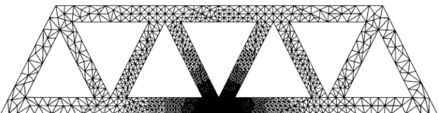
Ž . Figure 6. The test sampleTruss 7325 nodes, 14024 elements .
4. Performance evaluation and experimental results
We have implemented the PCMPLB method on an SP2 parallel machine and compared its performance with two load-balancing methods, the directed diffusion
Ž .w x Ž .w x
method DD 45 and the multilevel diffusion method MD 45 , and five mapping
w x w x
methods, the AErMC method 8 , the AErORB method 8 , the JOSTLE-MS
w x w x w x
method 45 , the MLkP method 24 , and the PARTY library method 35 . Three criteria, the execution time of mappingrload-balancing methods, the computation time of an application program under different mappingrload-balancing methods, and the speedups achieved by the mappingrload-balancing methods for an applica-tion program, are used for the performance evaluaapplica-tion.
In dealing with the unstructured finite element graphs, the distributed irregular
Ž . w x
mesh environment DIME 48 is used. DIME is a programming environment for doing distributed calculations with unstructured triangular meshes. The mesh covers a two-dimensional manifold, whose boundaries may be defined by straight lines, arcs of circles, or Bezier cubic sections. It also provides functions for creating, manipulating, and refining unstructured triangular meshes. Since the number of nodes in an unstructured triangular mesh cannot be over 10,000 in DIME, in this paper, we only use DIME to generate the initial test sample. From the initial test graph, we use our refining algorithms and data structures to generate the desired test graphs. The initial test graph used for the performance evaluation is shown in Figure 6. The number of nodes and elements for the test graph after each refinement are shown in Table 2. For the presentation purpose,
Table 2. The number of nodes and elements of the test graphTruss
Refinement Initial Ž . Samples 0 1 2 3 4 5 Truss Node噛 18407 23570 29202 36622 46817 57081 Element噛 35817 46028 57181 71895 92101 112494
the number of nodes and the number of finite elements shown in Figure 6 are less than those shown in Table 2.
To emulate the execution of a solution-adaptive finite element application program on an SP2 parallel machine, we have the following steps. First, we read the initial finite element graph. Then we use the AErMC method, the AErORB method, the JOSTLE-MS method, the MLkP method, or the PARTY library method to map nodes of the initial finite element graph to processors. After the mapping, the computation of each processor is carried out. In our example, the
Ž .
computation is to solve Laplaces’s equation Laplace solver . The algorithm of
w x
solving Laplaces’s equation is similar to that of 2 . Since it is difficult to predict the number of iterations for the convergence of a Laplace solver, we assume that the maximum number of iterations executed by our Laplace solver is 1000. When the computation is converged, the first refined finite element graph is read. To balance the computational load of processors, the AErMC method, the AErORB method, the JOSTLE-MS method, the MLkP method, the PARTY library method, the directed diffusion method, the multilevel diffusion method, or the PCMPLB method is applied. After a mappingrload-balancing method is performed, the computation for each processor is carried out. The mesh refinement, load balanc-ing, and computation processes are performed in turn until the execution of a solution-adaptive finite element application program is completed.
By combining the initial mapping methods and methods for load balancing, there are twenty methods used for the performance evaluation. We defined Ms
AErMC, AErORB, JOSTLE-MS, MLkP, PARTY, AErMCrDD, AErORBrDD, JOSTLE-MSrDD, MLkPrDD, PARTYrDD, AErMCrMD, A ErO R BrM D , J O S T L E -M SrM D , M LkPrM D , P A R T YrM D , A ErM CrP C M P L B , A ErO R BrP C M P L B , JO STL E -M SrP C M P L B ,
4
MLkPrPCMPLB, PARTYrPCMPLB . In M, AErORB means that the AErORB method is used to perform the initial mapping and the AErORB method is used to balance the computational load of processors in each refine-ment. AErORBrPCMPLB means that the AErORB method is used to perform the initial mapping and the PCMPLB method is used to balance the computational load of processors in each refinement.
4.1. The cost model for mapping unstructured solution-adapti¨e finite element models on distributed memory multicomputers
To map an N-node finite element graph on a P-processor distributed memory multicomputer, we need to assign nodes of the graph to processors of the multicomputer. There are PN mappings. The execution time of a finite element
graph on a distributed memory multicomputer under a particular mappingr load-balancing method Li can be defined as follows:
Ž .
where Tp ar Li is the execution time of a finite element application program on a
Ž .
distributed memory multicomputer under Li,Tc o m p Li,Pj is the computation cost
Ž .
of processor Pj under Li, andTc o m m Li,Pj is the communication cost of processor
Pj under Li, where is1, . . . ,PN and js0, . . . ,Py1.
The cost model used in Equation 1 is assuming a synchronous communication mode in which each processor goes through a computation phase followed by a communication phase. Therefore, the computation cost of processor Pj under a mappingrload-balancing method Li can be defined as follows:
Tc o m p
Ž
Li,Pj.
sS=load PiŽ
j.
=Tt a sk,Ž .
2 where S is the number of iterations performed by a finite element method,Ž .
load Pi j is the number of nodes of a finite element graph assigned to processor Pj, andTt a sk is the time for a processor to execute a task.
In our communication model, we assume that every processor can communicate with all other processors in one step. In general, it is possible to overlap the
Ž .
communication with the computation. In this case, Tc o m m Li,Pj may not always reflect the true communication cost since it could be partially overlapped with that
Ž .
of the computation. However, Tc o m m Li,Pj can provide a good estimate for the communication cost. Since we use a synchronous communication mode,
Ž .
Tc o m m Li,Pj can be defined as follows:
Tc o m m
Ž
Li,Pj.
sS=Ž
␦=Ts et u pq=Tc.
,Ž .
3 whereS is the number of iterations performed by a finite element method,␦ is the number of processors that processor Pj has to send data to in each iteration,Ts et u pis the setup time of the IrO channel, is the total number of bytes that processor
Pj has to send out in each iteration, and Tc is the data transmission time of the IrO channel per byte.
Let Ts e q denote the execution time of a finite element graph on a distributed memory multicomputer with one processor. The speedup resulted from a map-pingrload-balancing method Li for an application program is defined as
Ts e q
Speedup L
Ž
i.
s ,Ž .
4Tp ar
Ž
Li.
Ž .
LetT Li denote the time for the Laplace solver to execute one iteration for the
ith refinement of the test finite element graph under a mappingrload-balancing method, where is0, 1, . . . , 5 and LgM. For the presentation purpose, we assume that the initial finite element graph is the 0th refined finite element graph.
Ž .
T Li is defined as follows:
The total execution time of test finite element graphs on a distributed memory multicomputer is defined as follows:
5
Tt o t al
Ž
L.
sTe x ecŽ
L.
qÝ
T LiŽ
.
=Si,Ž .
6is0
Ž .
where Tt o t al L is the total execution time of the test samples under a mappingrload-balancing method L on a distributed memory multicomputer, Lg
Ž .
M,Te x ec L is the total execution time of a mappingrload-balancing method L
for test samples, and Si is the number of iterations executed by the Laplace solver for the ith refinement. From Equation 6, we can derive the speedup achieved by a mappingrload-balancing method as follows:
Ý5is0Seqi=Si
Speedup L
Ž
.
s 5 ,Ž .
7Te x ec
Ž
L.
qÝis0T LiŽ
.
=SiŽ .
whereSpeedup L is the speedup achieved by a mappingrload-balancing Lfor test samples, LgM, and Seqi is the time for the Laplace solver to execute one iteration for the ith refinement of test graphs in sequential.
The maximum speedup achieved by a mappingrload-balancing Lcan be derived Ž .
by setting the value of Si to ⬁. In this case, Te x ec L is negligible. We have the following equation:
Ý5is0Seqi
Speedupma x
Ž
L.
s 5 .Ž .
8Ýis0T Li
Ž
.
Ž .where Speedupma x L is the maximum speedup achieved by mappingr load-balanc-ing Land LgM.
4.2. Comparisons of the execution time of mappingrload-balancing methods
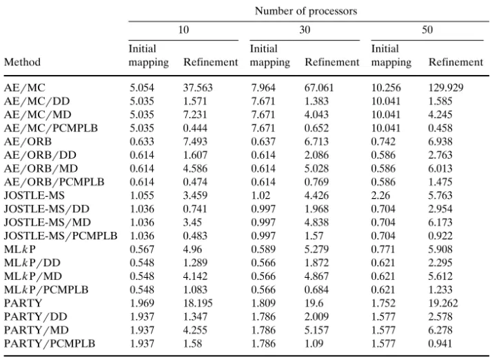
The execution times of different mappingrload-balancing methods for Truss on the 10, 30, and 50 processors of an SP2 parallel machine are shown in Table 3. In Table 3, we list the initial mapping time and the refinement time for mappingrload-balancing methods. The initial mapping time is the execution time of mapping methods to map finite element nodes of the initial test sample to processors. The refinement time is the sum of the execution time of mappingrload-balancing methods to balance the load of processors after each refinement. Since we deal with the load balancing issue in this paper, we will focus on the refinement time comparison of mappingrload-balancing methods. From Table 3, we can see that, in general, the refinement time of load-balancing
Ž .
methods is less than that of the mapping methods. The reasons are 1 the mapping methods have a higher time complexity than those of the load-balancing methods;
Table 3. The execution time of different mappingrload-balancing methods for the test sample on different numbers of processors
Number of processors
10 30 50
Initial Initial Initial
Method mapping Refinement mapping Refinement mapping Refinement
AErMC 5.054 37.563 7.964 67.061 10.256 129.929 AErMCrDD 5.035 1.571 7.671 1.383 10.041 1.585 AErMCrMD 5.035 7.231 7.671 4.043 10.041 4.245 AErMCrPCMPLB 5.035 0.444 7.671 0.652 10.041 0.458 AErORB 0.633 7.493 0.637 6.713 0.742 6.938 AErORBrDD 0.614 1.607 0.614 2.086 0.586 2.763 AErORBrMD 0.614 4.586 0.614 5.028 0.586 6.013 AErORBrPCMPLB 0.614 0.474 0.614 0.769 0.586 1.475 JOSTLE-MS 1.055 3.459 1.02 4.426 2.26 5.763 JOSTLE-MSrDD 1.036 0.741 0.997 1.968 0.704 2.954 JOSTLE-MSrMD 1.036 3.45 0.997 4.838 0.704 6.173 JOSTLE-MSrPCMPLB 1.036 0.483 0.997 1.57 0.704 0.922 MLkP 0.567 4.96 0.589 5.279 0.771 5.908 MLkPrDD 0.548 1.289 0.566 1.872 0.621 2.295 MLkPrMD 0.548 4.142 0.566 4.867 0.621 5.612 MLkPrPCMPLB 0.548 1.083 0.566 0.684 0.621 1.233 PARTY 1.969 18.195 1.809 19.6 1.752 19.262 PARTYrDD 1.937 1.347 1.786 2.009 1.577 2.578 PARTYrMD 1.937 4.255 1.786 5.157 1.577 6.278 PARTYrPCMPLB 1.937 1.58 1.786 1.09 1.577 0.941
Time unit: seconds
Ž .
and 2 the mapping methods need to perform gather-scatter operations that are time consuming in each refinement.
For the same initial mapping method, the refinement time of the PCMPLB method, in general, is less than that of the directed diffusion and the multilevel diffusion methods. The reasons are as follows:
Ž .1 The PCMPLB method has less time complexity than those of the directed diffusion and the multilevel diffusion methods.
Ž .2 The number of data movement steps among processors in the PCMPLAB method is less than those of the directed diffusion method and the multilevel diffusion method.
4.3. Comparisons of the execution time of the test sample under different mappingr load-balancing methods
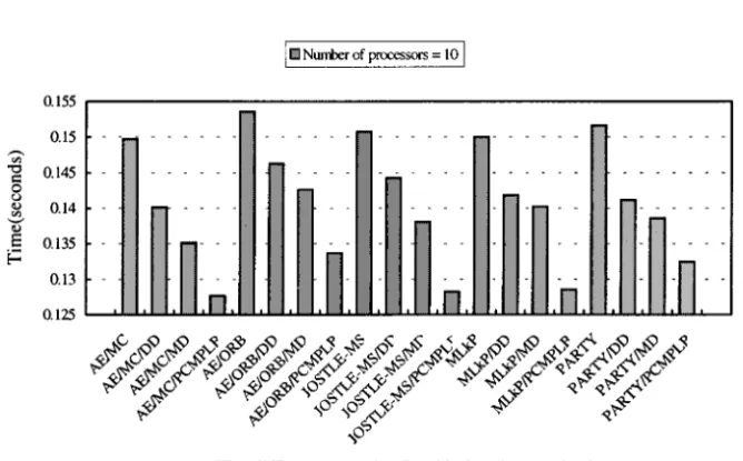
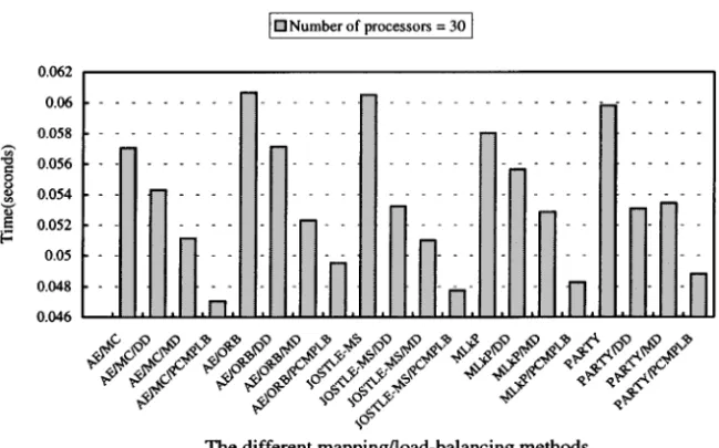
Ž
The times for a Laplace solver to execute one iteration computationq .
meth-ods on the 10, 30, and 50 processors of an SP2 parallel machine are shown in Figure 7, Figure 8, and Figure 9, respectively. Since we assume a synchronous communication model, the total time for a Laplace solver to complete its job is the sum of the computation time and the communication time. From Figure 7 to Figure 9, we can see that if the initial mapping is performed by a mapping method Žfor example AErORB and the same mapping method or a load-balancing.
Ž .
method DD, MD, PCMPLB is performed for each refinement, the execution time of a Laplace solver under the proposed load-balancing method is less than that of other methods. The reasons are as follows:
Ž .1 In the PCMPLB method, data migration is done between adjacent processors. This local data migration mechanism can reduce the communication cost of a Laplace Solver.
Ž .2 The PCMPLB method can fully balance the load of processors. In JOSTLE-MS, MLkP, and PARTY, 3%᎐5% load imbalance are allowed due to the trade-off between the computation and the communication costs. The DD and MD methods may not be able to balance the load of processors sometimes. This load imbalance may result in high computation cost.
Ž .
Figure 7. The time for Laplace solver to execute one iteration computationqcommunication for the test sample under different mappingrload-balancing methods on 10 processors.
Ž . Figure 8. The time for Laplace solver to execute one iteration computationqcommunication for the test sample under different mappingrload-balancing methods on 30 processors.
Ž .
Figure 9. The time for Laplace solver to execute one iteration computationqcommunication for the test sample under different mappingrload-balancing methods on 50 processors.
4.4. Comparisons of the speedups under the mappingrload-balancing methods for the test sample
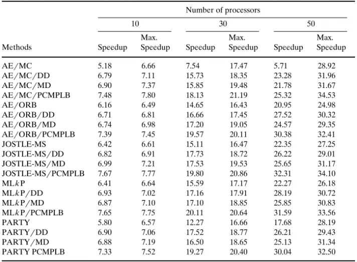
The speedups and the maximum speedups under the mappingrload-balancing methods on the 10, 30, and 50 processors of an SP2 parallel machine for the test sample are shown in Table 4. From Table 4, we can see that if the initial mapping
Ž .
is performed by a mapping method for example AErORB and the same mapping
Ž .
method or a load-balancing method DD, MD, PCMPLB is performed for each refinement, the proposed load-balancing method has the best speedup among mappingrload-balancing methods.
From Table 4, we can also see that if the initial mapping is performed by a
Ž .
mapping method for example AErORB and the same mapping method or a
Ž .
load-balancing method DD, MD, PCMPLB is performed for each refinement, the proposed load-balancing method has the best maximum speedup among mappingrload-balancing methods. For the mapping methods, AErMC has the best maximum speedups for test samples. For the load-balancing methods, AErMCrPCMPLB has the best maximum speedups for test samples. From Table 4, we can see that if a better initial mapping method is used, a better maximum speedup can be expected when the PCMPLB method is used in each refinement.
Table 4. The speedups and maximum speedups for the test sample under the mappingrload-balancing methods on an SP2 parallel machine
Number of processors
10 30 50
Max. Max. Max.
Methods Speedup Speedup Speedup Speedup Speedup Speedup
AErMC 5.18 6.66 7.54 17.47 5.71 28.92 AErMCrDD 6.79 7.11 15.73 18.35 23.28 31.96 AErMCrMD 6.90 7.37 15.85 19.48 21.78 31.67 AErMCrPCMPLB 7.48 7.80 18.13 21.19 25.32 34.53 AErORB 6.16 6.49 14.65 16.43 20.95 24.98 AErORBrDD 6.71 6.81 16.66 17.45 27.52 30.32 AErORBrMD 6.74 6.98 17.20 19.05 24.57 29.35 AErORBrPCMPLB 7.39 7.45 19.57 20.11 30.38 32.41 JOSTLE-MS 6.42 6.61 15.11 16.47 22.35 27.25 JOSTLE-MSrDD 6.82 6.91 17.73 18.72 26.22 29.01 JOSTLE-MSrMD 6.99 7.21 17.53 19.53 25.65 31.17 JOSTLE-MSrPCMPLB 7.67 7.77 19.80 20.86 32.31 34.10 MLkP 6.41 6.64 15.59 17.17 22.27 26.18 MLkPrDD 6.93 7.02 17.16 17.91 28.19 30.72 MLkPrMD 6.87 7.10 17.10 18.85 25.85 30.83 MLkPrPCMPLB 7.65 7.75 20.11 20.64 31.59 33.56 PARTY 5.80 6.57 12.27 16.66 17.68 28.19 PARTYrDD 6.90 7.06 17.52 18.77 26.21 29.43 PARTYrMD 6.88 7.19 16.50 18.65 25.13 31.34 PARTY PCMPLB 7.33 7.52 19.27 20.40 30.04 32.50
5. Conclusions
In this paper, we have proposed a prefix code matching parallel load balancing method, the PCMPLB method, to deal with the load unbalancing problems of solution-adaptive finite element application programs. We have implemented this method on an SP2 parallel machine and compared its performance with two load-balancing methods, the directed diffusion method and the multilevel diffusion method, and five mapping methods, the AErMC method, the AErORB method, the JOSTLE-MS method, the MLkP method, and the PARTY library method. An unstructured finite element graph Truss was used as the test sample. Three criteria, the execution time of mappingrload-balancing methods, the execution time of a solution-adaptive finite element application program under different mappingrload-balancing methods, and the speedups under mappingr load-balanc-ing methods for a solution-adaptive finite element application program, are used
Ž . for the performance evaluation. The experimental results show that 1 if a mapping method is used for the initial partitioning and this mapping method or a load-balancing method is used in each refinement, the execution time of an application program under a load-balancing method is shorter than that of the
Ž .
mapping method. 2 The execution time of an application program under the PCMPLB method is shorter than that of the directed diffusion method and the multilevel diffusion method.
Acknowledgments
The authors would like to thank Dr. Robert Preis, Professor Karypis, and Professor Chris Walshaw for providing the PARTY, the METIS, and JOSTLE software packages.
The work of this paper was partially supported by the National Science Council of Republic of China under contract NSC-87-2231-E-035-010.
References
1. I. G. Angus, G. C. Fox, J. S. Kim, and D. W. Walker.Sol¨ing Problems on Concurrent Processors, Vol. 2. Prentice-Hall, Englewood Cliffs, N. J., 1990.
2. C. Aykanat, F. Ozguner, F. Ercal, and P. Sadayaooan. Iterative algorithms for solution of large¨
Ž .
sparse systems of linear equations on hypercubes. IEEE Trans. on Computers, 37 12 :1554᎐1568, 1988.
3. C. Aykanat, F. Ozguner, S. Martin, and S. M. Doraivelu. Parallelization of a finite element¨ application program on a hypercube multiprocessor.Hypercube Multiprocessor, 662᎐673, 1987. 4. S. B. Baden. Programming abstractions for dynamically partitioning and coordinating localized
scientific calculations running on multiprocessors.SIAM Journal on Scientific and Statistical Comput
-Ž .
ing, 12 1 :145᎐157, 1991.
5. S. T. Barnard and H. D. Simon. Fast multilevel implementation of recursive spectral bisection for
Ž .
6. S. T. Barnard and H. D. Simon. A parallel implementation of multilevel recursive spectral bisection for application to adaptive unstructured meshes. Proceedings of the Se¨enth SIAM Conference on Parallel Processing for Scientific Computing, pp. 627᎐632. San Francisco, Feb. 1995.
7. J. A. Bondy and U. S. R. Murty.Graph Theory with Applications. Elsevier North Holland, New York, 1976.
8. Y. C. Chung and C. J. Liao, A processor oriented partitioning method for mapping unstructured finite element models on SP2 parallel machines. Technical report. Institute of Information Engi-neering, Feng Chia University, Taichung, Taiwan, 1996.
9. G. Cybenko. Dynamic load balancing for distributed memory multiprocessors. Journal of Parallel Ž .
and Distributed Computing, 7 2 :279᎐301, 1989.
10. F. Ercal, J. Ramanujam, and P. Sadayappan. Task allocation onto a hypercube by recursive mincut bipartitioning. Journal of Parallel and Distributed Computing, 10:35᎐44, 1990.
11. C. Farhat and H. D. Simon. TOPrDOMDECᎏa software tool for mesh partitioning and parallel processing. Technical report RNR-93-011. NASA Ames Research Center, 1993.
12. C. M. Fiduccia and R. M. Mattheyes. A linear-time heuristic for improving network partitions.
Proceeding of the 19th IEEE Design Automation Conference, pp. 175᎐181, 1982.
13. M. R. Garey and D. S. Johnson.Computers and Intractability, A Guide to Theory of NP-Completeness. Freeman, San Francisco, 1979.
14. J. R. Gilbert and E. Zmijewski. A parallel graph partitioning algorithm for a message-passing
Ž .
multiprocessor. International Journal of Parallel Programming, 16 6 :427᎐449, 1987.
15. J. R. Gilbert, G. L. Miller, and S. H. Teng. Geometric mesh partitioning: implementation and experiments. Proceedings of 9th International Parallel Processing Symposium, pp. 418᎐427. Santa Barbara, Calif. Apr. 1995.
16. A. Heirich and S. Taylor. A Parabolic Load Balancing Method,Proceeding of ICPP’95, pp. 192᎐202, 1995.
17. B. Hendrickson and R. Leland. The Chaco user’s guide: version 2.0. Technical report SAND94-2692. Sandia National Laboratories, Albuquerque, NM, Oct. 1994.
18. B. Hendrickson and R. Leland. An improved spectral graph partitioning algorithm for mapping
Ž .
parallel computations.SIAM Journal on Scientific Computing, 16 2 :452᎐469, 1995.
19. B. Hendrickson and R. Leland. An multilevel algorithm for partitioning graphs. Proceeding of Supercomputing’95, Dec. 1995.
20. G. Horton. A multi-level diffusion method for dynamic load balancing. Parallel Computing, 19:209᎐218, 1993.
21. S. H. Hosseini, B. Litow, M. Malkawi, J. Mcpherson, and K. Vairavan. Analysis of a graph coloring based distributed load balancing algorithm. Journal of Parallel and Distributed Computing,
Ž .
10 2 :160᎐166, 1990.
22. Y. F. Hu and R. J. Blake. An optimal dynamic load balancing algorithm. Technical report DL-P-95-011. Daresbury Laboratory, Warrington, UK, 1995.
23. D. A. Huffman. A method for the construction of minimum redundancy codes. Proceedings of the IRE 40, pp. 1098᎐1101, 1952.
24. G. Karypis and V. Kumar. Multilevel k-way partitioning scheme for irregular graphs. Technical report 95-064. Department of Computer Science, University of Minnesota, Minneapolis, 1995. 25. G. Karypis and V. Kumar. A fast and high quality multilevel scheme for partitioning irregular
graphs. Technical report 95-035. Department of Computer Science, University of Minnesota, Minneapolis, 1995.
26. B. W. Kernigham and S. Lin. An efficient heuristic procedure for partitioning graphs. Bell Syst.
Ž .
Tech. J. 49 2 :292᎐370, 1970.
27. L. Lapidus and C. F. Pinder. Numerical Solution of Partial Differential Equations in Science and Engineering. Wiley, New York, 1983.
28. F. C. H. Lin, and R. M. Keller. The gradient model load balancing method.IEEE Trans.Software Ž .
Engineering, SE-13 1 :32᎐38, 1987.
29. D. M. Nicol. Rectilinear partitioning of irregular data parallel computations.Journal of Parallel and Ž .
Distributed Computing, 23 2 :119᎐134, 1994.
30. L. Oliker and R. Biswas. Efficient load balancing and data remapping for adaptive grid calculations. Technical report, NASA Ames Research Center, Moffett Field, Calif., 1997.
31. C. W. Ou, S. Ranka, and G. Fox. Fast and parallel mapping algorithms for irregular problems.The Ž .
Journal of Supercomputing, 10 2 :119᎐140, 1996.
32. C. W. Ou and S. Ranka. Parallel incremental graph partitioning. IEEE Trans. Parallel and Ž .
Distributed Systems, 8 8 :884᎐896, 1997.
33. F. Pellegrini and J. Roman. Scotch: a software package for static mapping by dual recursive bipartitioning of process and architecture graphs.Proceedings of HPCN’96, pp. 493᎐498, Apr. 1996. 34. J. R. Pilkington and S. B. Baden. Dynamic partitioning of non-uniform structured workloads with
Ž .
spacefilling curves. IEEE Trans.Parallel and Distributed Systems, 7 3 :288᎐300, 1996.
35. R. Preis and R. Diekmann. The PARTY partitioningᎏlibrary user guideᎏversion 1.1. Heniz Nexdorf Institute Universitat, Paderborn, Germany, Sep. 1996.¨
36. S. Ranka, Y. Won, and S. Sahni. Programming a hypercube multicomputer. IEEE Software,
Ž .
5 5 :69᎐77, 1988.
37. K. Schloegel, G. Karypis, and V. Kumar. Parallel multilevel diffusion algorithms for repartitioning of adaptive meshes. Technical report噛97-014. University of Minnesota, Department of Computer Science and Army HPC Center, 1997.
38. K. Schloegel, G. Karypis, and V. Kumar. Multilevel diffusion schemes for repartitioning of adaptive meshes. Technical report噛97-013. University of Minnesota, Department of Computer Science, Jun. 1997.
Ž .
39. W. Shu and M. Y. Wu. Runtime incremental parallel scheduling RIPS on distributed memory
Ž .
computers.IEEE Trans.Parallel and Distributed Systems, 7 6 :637᎐649, 1996.
40. W. Shu and M. Y. Wu. The direct dimension exchange method for load balancing in k-aryn-cubes.
Proceedings of Eighth IEEE Symposium on Parallel and Distributed Processing, pp. 366᎐369, New Orleans, Oct. 1996.
41. H. D. Simon. Partitioning of unstructured problems for parallel processing.Computing Systems in Ž .
Engineering, 2 2r3 :135᎐148, 1991.
42. C. H. Walshaw and M. Berzins. Dynamic load-balancing for PDE solvers on adaptive unstructured
Ž .
meshes.Concurrency: Practice and Experience, 7 1 :17᎐28, 1995.
43. C. H. Walshaw, M. Cross, and M. G. Everett. A localized algorithm for optimizing unstructured
Ž .
mesh partitions.The International Journal of Supercomputer Applications, 9 4 :280᎐295, 1995. 44. C. Walshaw, M. Cross, and M. G. Everett. Dynamic mesh partitioning: a unified optimisation and
load-balancing algorithm. Technical Report 95rIMr06. University of Greenwich, London, SE18 6PF, UK, Dec. 1995.
45. C. Walshaw.The Jostle User Manual:Version 2.0. University of Greenwich, London, UK, July, 1997. 46. M. Willebeek-LeMair and A. P. Reeves. Strategies for dynamic load balancing on highly parallel
Ž .
computers.IEEE Trans.Parallel and Distributed Systems, 4 9 :979᎐993, 1993.
47. R. D. Williams. Performance of dynamic load balancing algorithms for unstructured mesh
calcula-Ž .
tions.Councurrency: Practice and Experience, 3 5 :457᎐481, 1991.
48. R. D. Williams. DIME: Distributed Irregular Mesh En¨ironment. California Institute of Technology, 1990.
49. M. Y. Wu. On runtime parallel scheduling for processor load balancing. IEEE Trans. Parallel and Ž .
Distributed Systems, 8 2 :173᎐186, 1997.
50. C. Z. Xu and F. C. M. Lau. Analysis of the generalized dimension exchange method for dynamic
Ž .
load balancing. Journal of Parallel and Distributed Computing, 16 4 :385᎐393, 1992.
51. C. Z. Xu and F. C. M. Lau. The generalized dimension exchange method for load balancing ink-ary
Ž .