w or k i ng pa p ers
16 | 2011
June 2011
The analyses, opinions and fi ndings of these papers represent the views of the authors, they are not necessarily
those of the Banco de Portugal or the Eurosystem MOMENT CONDITIONS MODEL AVERAGING WITH AN
APPLICATION TO A FORWARD-LOOKING MONETARY POLICY REACTION FUNCTION
Luis F. Martins
Please address correspondence to Banco de Portugal Av. Almirante Reis 71, 1150-012 Lisboa, Portugal; [email protected]
BANCO DE PORTUGAL Av. Almirante Reis, 71 1150-012 Lisboa
www.bportugal.pt
Edition
Economics and Research Department
Pre-press and Distribution Administrative Services Department Documentation, Editing and Museum Division Editing and Publishing Unit
Printing
Administrative Services Department Logistics Division Lisbon, June 2011 Number of copies 150 ISBN 978-989-678-085-2 ISSN 0870-0117 (print) ISSN 2182-0422 (online)
Moment Conditions Model Averaging with an
Application to a Forward-Looking Monetary
Policy Reaction Function
Luis F. Martins
Department of Quantitative Methods and UNIDE, ISCTE-IUL, Portugal ([email protected]) This version: October 3rd, 2009
Abstract
In this paper, we examine the empirical validity of the baseline version of the forward-looking monetary policy reaction function proposed by Clarida, Gali, and Gertler (2000). For that purpose, we propose a moment conditions model averaging estimator in the Generalized Method of Moments and Generalized Empirical Likelihood setups. We derive some of their asymptotic properties under correctly speci…ed and misspeci…ed models. Although the model averaging estimates and the standard procedures point to a stabilizing policy rule during the Paul Volcker and Alan Greenspan tenures but not so during the pre-Volker period, our results cast serious doubts on the signi…cance of the cyclical output variable as a forcing variable in the FED funds dynamics during the Volcker-Greenspan period.
Keywords: Forward-Looking Monetary Policy Rule; Stabilizing Policy; Generalized Method of Moments; Generalized Empirical Likelihood; Model Selection; Model Averaging; Misspeci…cation
JEL Classi…cation: C22; C52; E43; E52
This study was conducted while the author was visiting the Economics and Research Department (ERD) for a short-term scholarship. The author acknowledges …nancial support from the ERD, Portuguese Central Bank (PCB), and thanks its members for useful comments. The analysis, opinions and …ndings of this paper represent the views of the author, they are not necessarily those of the PCB or the Eurosystem.
1
Introduction
The forward-looking monetary policy reaction function proposed by Clarida, Gali, and Gertler (2000, henceforth CGG), based on Clarida, Gali, and Gertler (1998), has become a fundamental macroeconomic speci…cation in the context of the United States monetary policy in the postwar. In this model, the central bank forms beliefs about the future state of the economy based on the available information so far. The target rate depends on the expected in‡ation and output gaps with respect to their equilibrium values. Moreover, the monetary authorities do not immediately set the actual interest rate to its targeted counterpart but rather adjusts it smoothly over time. They employ the Generalized Method of Moments (GMM) methodology to estimate the monetary policy using the Federal Funds rate as the instrument of policy making1. In particular,
they suggest that the FED monetary policy during the Paul Volcker and Alan Greenspan period was more stable than during the …fteen or so years prior to Volcker’s appointment. The reasoning for this claim is that the Volcker-Greenspan policy appeared to be much more sensitive to changes in the expected in‡ation.
In this study, we re-evaluate the empirical validity of the baseline model discussed by CGG. For that purpose, we propose a new estimation method, which we call moment conditions model averaging estimator, in the GMM and Generalized Empirical Likelihood (GEL) setups. For completeness, we also employ existent moment and model selection criteria methods and the Empirical Likelihood (EL) estimation approach. We do so for several reasons. First, the CGG papers rely on a standard two-step GMM estimator, which may deviate substantially from its small sample distribution - as discussed in Hansen, Heaton and Yaron (1996), for example, and
in the two special issues of the Journal of Business and Economic Statistics (1996, vol. 14(3)
and 2002, vol. 20(4)) dedicated to GMM. Furthermore, the GMM estimation is not invariant to the speci…cation of the moment conditions, which means that the results depend on the normalization adopted for the estimation. Another drawback is that the results hinge on the weighting matrix used in the estimation2.
Given these disappointing properties of GMM, it has recently been proposed the GEL class 1There has been a considerable interest in the properties of the GMM estimator to the analysis of time series
dependent data. In fact, since the seminal contribution by Hansen (1982), one has witnessed the remarkable growth of the theoretical and empirical research on this issue over the recent decades. One of the main reasons why it became so popular in moment conditions models is its computational accessibility.
2In CGG paper, it is not clear what weighting matrix is used. If by "optimal" they mean the HAC matrix
of estimators. Newey and Smith (2004) have shown that while GMM and GEL estimators have identical …rst-order asymptotic properties, the latter are higher order e¢ cient, in the sense that these estimators are able to eliminate some sources of GMM biases. For example, they show that the bias of the EL estimator does not grow with the number of moment conditions, unlike GMM. Similar properties have been established by Anatolyev (2005), in a time series setting.
The second main reason for re-evaluating the empirical results by CGG concerns the econo-metric analysis of model selection in the context of moment condition models. In the standard GMM and GEL estimation approaches (as in CGG, for the case of GMM), parameter estimates are obtained with a given/…xed list of instruments (moment conditions, in general). On the other hand, in model selection, one ranks the available moment conditions models (combina-tions of instruments, in the linear IV case) according to the particular goal undertaken. Instead of just one, in model selection there are "many" competing models.
Model selection based on information criteria, hypothesis testing or shrinkage-type estimat-ors has already been studied in the GMM and GEL framework. See, for example, Smith (1992) and Smith and Ramalho (2002) for model testing and Caner (2009) for a LASSO-type GMM estimator. Out of these three lines of model selection research, we only apply the information criteria to the CGG model. Based upon the evidence that the rejection of the J-statistic is an indicator that some moment conditions are invalid, Andrews (1999) conceived a GMM inform-ation criteria procedure for consistently selecting the correct moment conditions. Andrews and Lu (2001) extend Andrews’paper to the case of jointly picking the moments and the parameter (model) vector, that is, imposing zero restrictions on the parameters. Hong, Preston and Shum (2003) extend these two previous papers to the GEL framework. Hall, Inoue, Jana and Shin (2007) take a di¤erent approach: The information criteria used for moment selection is based on the entropy of the limiting distribution of the GMM estimator.
We pursue an alternative methodological direction in model selection – Model Averaging (MA). In MA the estimation procedure is based on a weighted combination of all candidate models/estimators. The weights are chosen according to some relevant criterion. To smooth estimators across several models is a neat strategy to improve the bias and variance balance. Studies on least squares (Hansen, 2005), likelihood-based (see, for example, Hjort and Claeskens, 2003) and Bayesian (see, for example, Hoeting, Madigan, Raftery and Volinsky, 1999) MA have already been developed. At the notable study of Bruce Hansen, in the regression setup, it is through the well-known Mallows criterion that the weights are estimated. To our best knowledge, there is no published work yet in GMM/GEL MA estimators.
Thus, we propose GMM and GEL model averaging estimators and discuss some of their asymptotic properties under correctly speci…ed and misspeci…ed models. We show that the MA GMM asymptotic theory under misspeci…cation is not standard in the sense that the consistency and distributional results depend on the weighting matrices and the pseudo-true values. The optimal MA weights are found by means of particular moment and model selection criteria as de…ned at Andrews (1999), Andrews and Lu (2001), Hong, Preston and Shum (2003) and Hall et all (2007).
Although the MA estimates and the standard procedures point to the same conclusion, which is the evidence for a stabilizing policy rule during the Paul Volcker and Alan Greenspan tenures but not so during the pre-Volker period with respect to in‡ation, our results raise serious doubts on the signi…cance of the cyclical output variable as a forcing variable in the FED funds dynamics during the Volcker-Greenspan period. Contrary to our results, CGG found that the parameter associated with output gap was statistical signi…cant for most of the policy rule speci…cations. Before us, Jondeau, Le-Bihan and Gallès (2004) also questioned this result at CGG using standard GMM, CU and MLE methods.
In the next two sections, we brie‡y review the forward-looking monetary policy rule pro-posed by CGG and the econometrics of moment conditions models. In Section 4, we discuss the existence of a linear combination of instruments that give rise to a GMM/GEL estimator that attains the Chamberlain e¢ ciency bound relative to the set of all available instruments. The approach on moment conditions model averaging is presented in Section 5. The empirical application of the existing methods and the MA procedure to the baseline CGG model is in Section 6 and a conclusion …nalizes this paper.
2
Forward-Looking Monetary Policy Reaction Function
In order to provide a strong empirical evidence that the FED monetary policy during the Paul Volcker and Alan Greenspan period was more stable than during the …fteen or so years prior to Volcker’s appointment, Clarida, Gali, and Gertler (2000), based on Clarida, Gali, and Gertler (1998), estimates a policy rule for which the central bank has forward-looking expectations. Due to this type of speci…cation, they used the GMM methodology to estimate the monetary policy with the Federal Funds rate as the instrument of policy making during the aforementioned periods. In this paper, we illustrate the merits of our approach on GMM model averaging using the CGG forward-looking speci…cation of the monetary policy. To better understand the main
aspects of model, we now discuss the monetary policy dynamics following their work in a very close manner3.
CGG derived the forward-looking monetary policy reaction function without specifying a central bank’s objective function that would lead to an optimal monetary instrument rule. The baseline policy rule for the target nominal interest rate (nominal Federal Funds rate) at period
t; it;is given by
it =i + (Et t;k ) + Etxt;q; (1)
where t;k is the percent change in the price level between periods t and t+k; expressed in
annual rates, andxt;qis a measure of the average output gap betweentandt+q:The output gap
is de…ned as the percent deviation between actual GDP and the corresponding target. Moreover, denotes the target for in‡ation and, by model construction,i is the desired nominal interest rate when both the in‡ation rate and output are expected to be at their target levels. Et is the
expectation operator conditional on the information set available at time t; t: Hence, Et t;k
should be read as E( t;kj t):
In this model, the central bank forms beliefs about the future state of the economy based on the available information so far. The target rate at period t; it; is a linear function of the expected in‡ation and output gaps with respect to their target levels. The interest rate policy rules tend to be stabilizing for >1 and for >0 (the monetary rules are more likely to be
destabilizing for 1and <0);as model (1) is equivalent to
rt =r + ( 1) (Et t;k ) + Etxt;q; (2)
wherer =i is the equilibrium real interest rate andrt =it Et t;k is the (ex-ante) real
interest rate target. Here, stability occurs as a result of low real interest rates which stimulate economic activity and in‡ation.
Another key feature of the model is that the monetary authorities do not immediately set the actual interest rate to its targeted counterpart. To be in line with the literature, let us assume that the actual interest rate deviate randomly from the target rate due to monetary shocks et;
such that Et 1et= 0;and that the adjustment goes smooth over time according to
(L)it= (1 )it +et; (3)
with the pth order autoregressive lag polynomial (L) = 1 1L ::: pLp and
1 (1) = 1+:::+ p: (4)
3
The partial adjustment of the actual rate to the target value is observed through the equation
it= 1it 1+:::+ pit p+ (1 )it +et; (5)
whereitdepends on a linear combination of its past values and on the current target rate (plus
a zero mean exogenous interest rate shock). The parameter is interpreted as the degree of
smoothing of interest rate changes.
The CGG policy reaction rule for it results from combining the target nominal policy (1)
and the partial adjustment model that adjusts it gradually towardsit;(5). Substituting terms,
yields
it= 1it 1+:::+ pit p+ (1 ) [ + Et t;k+ Etxt;q] +et; (6)
where
=i =r + (1 ) : (7)
By the law of iterated expectations, equation (6) can be written as
it= 1it 1+:::+ pit p+ (1 ) [ + t+k+ xt+q] +"t; (8)
where the innovation "t follows the process
"t=et (1 ) [ ( t+k Et t+k) + (xt+q Etxt+q)]: (9)
The most appropriate estimation method to the unknown quantities ; ; and is GMM
(or GEL, for that matter)4. Indeed, the forecast errors t+k Et t+k and xt+q Etxt+q are,
by construction, orthogonal to any variable at the information set t and, most likely,
correl-ated with t+k and xt+q: The instrumental variables zt that belong to t are, most probably,
correlated with pastit; t+k and xt+q;as well.
In this paper, we build upon theoretical results on averaging GMM (and GEL) estimators. In this sense, we take the scenario of studying a macroeconomic model but, for which, there is possibly not a unique set of instruments to estimate the unknown parameters. To …x ideas, let
p; qand kbe any given values. For a particular set of instrumentsi(collected in ami 1vector
zt(i))one can de…ne a speci…c model Mi with orthogonality conditions
E it 1it 1 ::: pit p (1 ) [ + t+k+ xt+q] zt(i) = 0; (10)
which most likely provide distinct GMM estimates for di¤erent i:
4In this model, is identi…able but not i and ;jointly (notice that is identi…ed through
t+k). Thus, with the argument that is of some interest in the characterization of the monetary policy, following CGG, the parameter of interest subject to estimation is andi is measured as the observed sample average.
3
Econometric Framework
In this section, we review the most important and well-established results regarding the GMM and GEL estimation procedures as well as the moment and model selection criteria in moment condition models.
3.1 Moment Conditions Model
LetMbe the collection of candidate moment conditions models. Here,Mis a countable/…nite
or an uncountable set and a modelMi belongs to the family of modelsM:Mi 2 M:The "true"
model may or may not be a member of M: Take any particular moment conditions model,
Mi;which, in our application, is characterized by a particular set of instruments (for example,
model (10) in CGG setup). When the number of instruments is large, it is possible that no value of the parameter vector simultaneously satis…es all the moment restrictions exactly in the population, resulting in a misspeci…ed model. Next, we distinguish a correctly speci…ed model from a misspeci…ed one, as in Hall and Inoue (2003).
Correctly Speci…ed Model Consider the estimation of ap-dimensional parameter vector
0 = ( 0;1; :::; 0;p)2 <p based on m p moment conditions of the form
E[g(yt; 0)] E[gt( 0)] = 0; (11)
for all t; where, usually, g(yt; 0) gt( 0) = "(xt; 0) zt for some set of variables xt and
instrumentsztsuch thatyt= (x0t; z0t)0:When"tis univariate,gt( 0) =zt"(xt; 0)andztism 1;
which, for the linear regression model,5
gt( 0) =zt yt x0t 0 and E[zt yt x0t 0 ] = 0: (12)
Due to linearity, gt( ) is most certainly an unbounded function in the data: sup y
0g(y; ) = 1
for any and any unit vector :
Them pJacobian matrix is de…ned as
G( 0) G=E @g(yt; ) @ 0 = 0 ! (13) 5There should be no confusion in terms of notation: In the general case, y
t is the set of all variables in the model; In the linear case,ytis the dependent variable andxtthe covariates. Similarly,xtat the monetary model is the economic variable "output gap" and not a prede…ned set of covariates.
and, under some regularity conditions, a CLT can be invoked: p T 1 T T X t=1 g(yt; 0) ! d !Nm(0; S( 0)); (14)
asT ! 1;where the long-run variance of the processfg(yt; 0)gis somem mpositive de…nite matrix S( 0) S = lim T!1V ar " T 1=2 T X t=1 g(yt; 0) # : (15)
In the linear case,
G=E ztx 0 t and S= limT !1V ar " T 1=2 T X t=1 zt yt x0t 0 # ; (16)
which, under no-dependence (martingale di¤erence sequence),
S= 0=E gt( 0)gt( 0)0 =E ztzt0"2t : (17)
De…nition 1 (Correctly speci…ed model): The model is said to be correctly speci…ed if there
exists a unique value 0 in <p such that
E[g(yt; 0)] = 0: (18)
In this de…nition, the orthogonality condition isE[g(yt; 0)] = 0 and the identi…cation con-dition (uniqueness) results fromG full-column ranked6.
Misspeci…ed Model De…nition 2 (Misspeci…ed model): A model is said to be misspeci…ed
if there is no value of which satis…es the orthogonality condition, that is,
E[g(yt; )] = ( ) (19)
where : ! <m such that k ( )k>0 for all 2 :
In the previous de…nition, E[g(yt; )] is assumed to be constant for all t (it rules out
mis-speci…cation due to structural instability). Also, m > pbecause ifm=p then there must exist
some value of such that E[g(yt; )] = 0: This is a non-local misspeci…cation as we are not
considering local misspeci…cation where E[g(yt; 0)] =T 1=2 ; 6= 0;say.
According to Schennach (2007), in a misspeci…ed model infkE[g(yt; )]k > 0; whereas for
linear models, Maasoumi and Phillips (1982) de…ne misspeci…cation by E(zt"t) = ": Chen,
6
In this paper,we are not considering the many and weak instruments issues in the linear IV model nor weak identi…cation in the general GMM estimation procedure.
Hong and Shum (2007), among others, de…ne a misspeci…ed model di¤erently. For each 2 ;
letP = PjRg(y; )dP = 0 be a nonparametric family of measures forywhich are consistent
with the moment conditions. Then, we can de…ne P =[ 2 P as the family of measures that
are compatible with the moment conditions model. The model P is misspeci…ed if the true
population distribution P0 2 P= (in fact, P and P are induced by g and should be read as Pg
and Pg;instead).
So that an extremum estimator has a well de…ned probability limit in a misspeci…ed model, we need to impose the following identi…cation condition.
Assumption 1 (Identi…cation for a misspeci…ed model): There exists a pseudo-true value
2 such that Q0( ) < Q0( );8 2 n f g; where Q0( ) is the population objective
function, that is,
= arg minQ0( ): (20)
Note that two di¤erent estimators may converge to di¤erent pseudo-values (due to two
di¤erent well-de…ned objective functions). Given the existence of ; we de…ne the following
quantities: ( ) =E[g(yt; )]; (21) G = E @g(yt; ) @ 0 = ! ; and S = lim T!1V ar " T 1=2 T X t=1 (g(yt; ) ) # (positive de…nite).
In the linear model, G =G: Under some conditions given at Hall and Inoue (2003),
p T 1 T T X t=1 (g(yt; ) ) ! d !Nm(0; S ); asT ! 1: (22)
When the number of moment conditions is large, it is possible that no value of
simultan-eously satis…es all the moment restrictions exactly in the population, resulting in a misspeci…ed model. Another reason for considering misspeci…cation stems from the fact that most models are only approximations to the underlying phenomena. Although the imperfections of the model can be, in some cases, avoided through the use of speci…cation tests, the consequences on estim-ation may have little impact on the results. Also, misspeci…ed (and parsimonious) models may have reasonable predictive properties. Just like in MLE, the object of interest is the pseudo-true value of the parameter vector, which may not be unique since distinct objective functions may be speci…ed.
3.2 Estimation Procedures
In order to estimate (consistently and e¢ ciently) the unknown quantities 0or ;we discuss the typical estimation procedures in moment condition models: GMM (IV for linear models), CUE
and GEL. For a sample of sizeT; de…ne the sample counterparts of the population moments as
b gT( ) = 1 T T X t=1 g(yt; );GbT ( ) = 1 T T X t=1 @g(yt; ) @ 0 and (23) b
ST( ) = (HAC formula. See Den Haan and Levin, 1996, for example).
For the linear model,
b gT ( ) = 1 T T X t=1 zt yt x0t and GbT( ) = 1 T T X t=1 ztx 0 t= Z0X T : (24)
The GMM estimator is de…ned as
bGM M;T (W) = arg min 2 bgT( )
0
WTbgT( ); (25)
where WT is a weighting matrix such that WT
p
! W;a positive de…nite matrix. When m > p;
the asymptotic variance of pT bGM M;T 0 depends on the plimWT = W: For the
two-step e¢ cient estimator, WT = SbT bF S
1
b
ST1; where bF S is a …rst-step consistent GMM
estimator (take WT =Im;for example):
bEGM M;T = arg min 2 bgT( )
0 b
ST1bgT( ); (26)
where the random matrix SbT p
!S; asT ! 1:The GMM estimator depends on the weighting
matrixSbT1which is in‡uenced by the choice made for a …rst step consistent estimator. To over-come this issue, the continuous-updating (CU-GMM) objective function contains the weighting
matrix as a function itself of the unknown :
bCU E;T = arg min 2 bgT( )
0b
ST ( )bgT( ); (27)
where SbT is the generalized inverse ofSbT:
Solving for at FOC of the GMM objective function for the linear model,
1 T T X t=1 ztx0t !0 WT 1 T T X t=1 zt yt x0t ! = 0; (28)
we obtain the IV estimator
For the time-series version, WT = SbT1 evaluated at bF S = ((X0Z) (Z0X)) 1(X0Z) (Z0y);
whereas for the homoskecedastic with an error variance of one and no-dependence cross-section version,WT = T1 PTt=1ztzt0
1
= ZT0Z 1 (…rst step estimator calculated using the inverse of an instrument cross product matrix as the weighting matrix).
Given the often disappointing small sample properties of the GMM estimator, alternative methods have been proposed recently such as those belonging to the GEL class of estimators. Newey and Smith (2004) demonstrate that, while GMM and GEL estimators have identical …rst-order asymptotic properties, the latter are able to eliminate some sources of GMM biases. In particular, the bias of the EL estimator does not grow with the number of moment conditions, unlike GMM. Similar properties have been recently established by Anatolyev (2005), in a time series setting. This author demonstrates that, in the presence of correlation in g(yt; ), the
smoothed GEL estimator of Kitamura and Stutzer (1997) is e¢ cient, obtained by smoothing the moment function with the truncated kernel, so that it solves the saddle point problem
bSGEL;T = arg min 2 2supT( ) 1 T TXKT t=KT+1 [ 0gtT ( )] (30) with gtT ( ) = 1 2KT + 1 KT X k= KT g(yt k; ): (31) Here, T ( ) =f : 0 gtT( )2O; t=KT + 1; :::; T KTg; (32)
where the open setO includes the zero number and is them 1vector of lagrange multipliers
each associated with the jth moment condition, j = 1; :::; m: Moreover, the real function :
< ! < is twice di¤erentiable and concave on O and de…nes the speci…c GEL estimator. When
(v) = (1 +v)2=2; the GEL estimator coincides with the CUE of Hansen et al (1996). If
(v) = ln(1 v)we have the EL estimator of Kitamura (1997), whereas (v) = exp(v)leads to
the ET case presented by Kitamura and Stutzer (1997). In thei:i:d: case, the Newey and Smith
(2004) GEL typology sets KT = 0: The SEL variant, in particular, removes important sources
of bias associated with the GMM, namely the correlation between the moment function and its derivative7, as well as third-order biases. Furthermore, Anatolyev (2005) shows that even when there is no serial correlation, using smoothing and an appropriate HAC weight matrix, as in Andrews (1991) or Newey and West (1994), leads to a reduction in estimation biases.
7
It has been shown that, under some regularity conditions, the GMM and the GEL estimators have some probability limit and converge in distribution to some random variable under a correct or misspeci…ed model. These results are summarized in the following lines.
Correctly Speci…ed Model Under correct model speci…cation, the estimators are
con-sistent: bGM M;T p
! 0 and bGEL;T p
! 0; as T ! 1: Also, the EGMM and the GEL are
(…rst-order) equivalent: p n 0 @ bT 0 b 1 A d !Np+m(0; diag(V; P)); (33) where V = G0S 1G 1 and P =S 1 S 1GV G0S 1: (34)
Recall that for linear IV, G=E(ztx0t) and S depends on the properties of fzt"tg fgtg: For
the GMM estimator with an arbitrary weighting matrix WT;
p
T bGM M;T 0
d
!N 0; G0W G 1 G0W SW G G0W G 1 : (35)
The EGMM estimator is e¢ cient in the sense that it attains the smallest asymptotic variance
over the class of GMM estimators with alternative weighting matrices WT for a given set of
moment conditions. Chamberlain (1987) shows that the EGMM estimator is semiparametrically e¢ cient, that is,
G0S 1G 1 = E xtzt0 S 1E ztx0t
1
(36) is the lower bound for the variance of any estimation procedure based solely on the information
E[g(yt; 0)] = 0 and with unknown distribution. The GEL estimator also attain this e¢ ciency bound. It can also be shown that adding moment conditions improves asymptotic e¢ ciency but it increases the small sample bias (and it can increase the small sample variance).
Misspeci…ed Model The limiting distribution theory of the GMM estimator under
mis-speci…cation is derived by Hall and Inoue (2003). Its importance can be justi…ed through the
rejection of the model using the J-statistic and the need to keep the whole set of moment
conditions. The combination of overidenti…cation and misspeci…cation leads to a GMM
estim-ator whose plim depends on the limit of the weigthing matrix and whose limiting distribution
depends on the limiting distribution of the elements of the weigthing matrix (its rate of conver-gence included). As a consequence, there is no one single limiting distribution theory for the
GMM estimator8. This fact has also been proved by Maasoumi and Phillips (1982) for the IV estimator in linear models and a particular weighting matrix - the matrix ZT0Z 1:
The identi…cation condition states that there exists (W) 2 such that Q0( (W)) <
Q0( );8 2 n f (W)g;whereQ0( ) =E[g(yt; )]0W E[g(yt; )]:That is, the GMM
estim-atorbT is consistent for the pseudo-true value
(W) = arg minE[g(yt; )]0W E[g(yt; )]; (37) where b Q( ) = 1 TJT ( ) =gbT ( ) 0 WTbgT ( ) p !E[g(yt; )]0W E[g(yt; )] =Q0( ) (38) uniformly in ;ifWT p !W:
Hall and Inuoe (2003) consider four cases, each with its own speci…c limiting
distribu-tion. Whenever WT =W for all T or
p
T(WT W) is asymptotically normal,
p
T bT
converges in distribution to a normal process with zero expectation and a variance that de-pends on several quantities and distinct from the correctly speci…ed model. The …rst case
includes the FS estimation, WT = Im; and the second case includes another FS estimator,
WT = T1 PTt=1ztzt0
1 p
! E(ztzt0) =W;and a second step estimator based on the assumption
that fzt(yt x0t ) g is a martingale di¤erence sequence,
WT = 1 T T X t=1 h zt yt x0tbT (1) b 1 i h zt yt x0tbT (1) b 1 i0! 1 (39)
where bT(1) denotes the GMM estimator on the …rst-step such that plimbT (1) = (1) and
bT (1) (1) = Op T 1=2 and b 1 =bgT bT(1) : In the third case, WT is the inverse of a
centred HAC estimator, WT =SbT bT (1)
1 ;where b ST bT (1) = TX1 i= T+1 !(i=bT)ei; (40) with ei= 8 < : 1 T PT t=i+1 h zt yt x0tbT (1) b 1 i h zt i yt i x0t ibT (1) b 1 i0 ; ifi 0 1 T PT t= i+1 h zt+i yt+i x0t+ibT(1) b 1 i h zt yt x0tbT (1) b 1 i0 ; ifi <0 (41)
Let (2) = S 1 : If the bandwidth does not increase too quickly, qbT
T bT (2) (2)
converges in distribution to a normal process with zero or non-zero expectation and a certain 8
The iterated GMM changes its distribution at each iteration! Also, inference on the pseudo-true values is troubling. Finally, we no longer have …rst-order equivalence.
variance; Otherwise, bkT bT
p
!constant (degenerates), where k > 0 is the characteristic exponent of the kernel. Finally, the case whereWT is the inverse of a uncentred HAC estimator:
bT bT converges in probability to a constant, in most of the cases.
Contrary to the GMM procedure, the limiting properties of the GEL class of estimators un-der misspeci…cation has not been fully un-derived yet. Recently, Schennach (2007) provides some results for the EL and the ET estimators under some speci…c conditions. She proves that the
EL estimator may cease to be pT-consistent in the i:i:d: setting under model misspeci…cation
and unbounded moment conditions (relevant for the linear IV estimator) even when their
ex-pectations are bounded. The objective functionQ0( )is a KLIC discrepancy measure for which
the EL pseudo-value does not exist becauselog 1 + 0g(yt; ) is ill-de…ned for unboundedg:
Without a non-zero ;one cannot de…ne a EL pseudo-true which satis…es the model moment
conditions. The existence and de…nition of a EL pseudo-true value for which the EL estimator converges is still to be discussed. For bounded conditions and misspeci…cation, pT-consistent of the EL estimator is possible.
In contrast, the ET estimator avoids this problem because, even with unbounded moments,
its objective does not restrict the values for :Therefore, the ET is more robust than EL
un-der misspeci…cation since their pseudo-true values are well-de…ned9. In her paper, Schennach
proposes a hybrid estimator, the so-called ETEL (Exponentially Tilted Empirical Likelihood), that combines the EL and the ET estimators to exhibit the advantages of both. Under
misspe-ci…cation, she shows that the ETEL avoids EL’s pitfalls maintaining root pT convergence with
pseudo-true values ( ; )that are generically well de…ned.
3.3 Moments and Model Selection Criteria
Due to the well-known bias/variance trade-o¤ in any estimation method, in this section we present the main existing results on how to choose among a …nite number of instruments/moment conditions in the GMM and GEL setup. Donald and Newey (2001) discuss on how to choose among a list of instruments in a system of linear simultaneous equations using the 2SLS and LIML instrumental variables estimators. In this setup, one chooses the (optimal) instruments, with the corresponding estimator, such that the estimated mean square error is minimized. In the GMM and GEL literature, the choice of moments is achieved according to some general
9
Schennach (2007) refers to a 2000 paper by Yuichi Kitamura to justify the existence of a …nite asymptotic variance at thepT-rate limiting distribution of the ET under misspeci…cation.
information criteria instead10. The procedures described below assume that the selected moment conditions (the correct model itself) is not misspeci…ed. On the other hand, the papers by Hall and Inoue (2003) and Schennach (2007) on misspeci…ed models do not treat the issue of model selection.
Based upon the evidence that the rejection of the J-statistic is an indicator that some
moment conditions are invalid, Andrews (1999) conceived a GMM procedure for consistently
selecting the correct moment conditions. Following his notation, let mdenote the total number
of available moment conditions and let the GMM moment selection criteria for a given model be de…ned as
M SCT (c) =JT(c) T(jcj p); (42)
wherec2 <mis a moment selection vector that represents a list of "selected" moment conditions
(subset ofg);jcjdenotes the cardinality (number) of the "selected" momentsc(jcj m); JT (c)is
theJ-statistic computed using the "selected" momentsc;jcj pis the number of overidentifying
restrictions and T = o(T) is a sequence that de…nes the selection criterion: T = 2 for the
AIC; T = logT for the BIC; and T =Qlog logT for some Q > 2 for the HQ-type criterion.
De…ning the unit-simplex set
C = c2 <mn f0g:cj = 0 or1;81 j m; wherec= (c1; :::; cm)0 ; (43)
c is a vector of zeros (excluded conditions) and ones (included conditions) and jcj=Pmj cj for
c2C:Accordingly, for a GMM estimator based on the moment conditions c;bT(c);
JT (c) =Tinf 2 bgT c( ) 0 WT(c)bgT c( ) =TbgT c bT (c) 0 WT (c)gbT c bT (c) ; (44)
where WT (c) is the jcj jcjweight matrix employed with the moment conditionsgbT c( ):
The moment selection criteria estimator is de…ned as b
cmsc= arg min
c2CM SCT(c) = arg minc2C (JT (c) T (jcj p)); (45)
where C C; with f0g 2 C; is some parameter space for the moment selection vector. The
estimator bcmsc picks the moment conditions c over C such that the increase in JT (c) that
typically occurs when moment conditions are added (even if correct) is o¤set by the "bonus term" T (jcj p) that rewards selection vectors that utilize more moment conditions. Under
1 0Quite often, empirical information criteria are used when proved to be consistent in choosing the correct
some technical conditions, Andrews (1999) shows thatbcis a consistent11estimator ofc0;assumed to be the single "correct" selection vector. If, additionally, one assumes thatE(gc0( )) = 0 has
a unique solution 0 2 (the "true" value of ;set atc0);thenbc consistently estimates bothc0
and 0:
At Andrews (1999), the selection of corrects moments is conditional on correct modeling. Andrews and Lu (2001) extend Andrews’paper to the case of jointly picking the moments and the parameter (model) vector, that is, imposing zero restrictions on the parameters. Now, let
(b; c) denote a pair of model and moment selection vectors andjbjandjcjdenote the number of
parameter from the vector (not necessarily all of them) and moments, respectively, selected
by (b; c):The MMSC selects the pair (b; c) that minimizes JT (b; c) T (jcj jbj);where
JT (b; c) =T inf [b]2 [b] b gT c [b] 0 WT (b; c)bgT c [b] =TbgT c bT (b; c) 0 WT(b; c)bgT c bT (b; c) : (46)
Here, bT (b; c) 2 [b] is the GMM estimator based on the model and moments selection
(b; c): It can be shown that the pair bbmmsc;bcmmsc is a consistent estimator. Hong, Preston
and Shum (2003) extend these two previous papers to the GEL framework: At the de…nition of MMSC, replace JT(b; c) by GELT(b; c) = 2Tmin [b] sup c 1 T TXKT t=KT+1 0 cgtT c( [b]) ; (47) where gtT c [b] = 2KT1+1 PKT k= KT gc yt k; [b] :
4
Model Averaging Instruments
So far, the literature on moment conditions models has essentially focused on estimation meth-ods fora given model and on optimally selectinga model among a list of candidate alternatives. In this section, we build upon the principle that gains can be obtained once we consider all the available moment conditions in hand and average them out to obtain an alternative estimator. Although the setup could be de…ned for generalgfunctions, we take the special case of linear IV moment conditions because averaging instruments makes the study more interesting and appeal-ing. After de…ning some key concepts and optimality criteria we present instrument averaging under correct and misspeci…ed models which, in this case, imply valid and invalid instruments. 1 1The GMM-AIC is not consistent and it has positive probability (even asymptotically) of selecting too few
If one is not willing to do instrument averaging without dropping invalid instruments, then previous to the analysis of model averaging under correct speci…cation one can do instruments selection as proposed by Andrews (1999), Andrews and Lu (2001) and Hong, Preston and Shum (2003).
4.1 De…nitions
For am-dimensional vectorzt; t= 1; :::; T of available (valid or invalid) instruments, withm p;
de…ne ap mmatrix z of p linear combinations of the instruments such thatzet = zt is
p-dimensional. De…ne the set of all possible instrument averages (up to a constant)
Zt=fzet :zte= zt; for somep m matrix such that 6= 0 and 11= 1g: (48)
For a well-de…ned criteria, the goal is to …nd an optimal weightbthat give rise to a selected vector b
zte2 Ztin a way that the estimation of an overidenti…ed system is reduced to one that is exactly
identi…ed. We build optimal instruments instead of selecting instruments (as in Andrews, 1999 and Donald and Newey, 2001, among others). In our optimality criteria, the resulting estimator ought to be consistent and, whenever possible, attain the Chamberlain e¢ ciency bound relative to the setzt:When averaging instruments we do not consider the standard information criteria
since all the instruments are assumed to be used: c= m (vector of ones) and jcj=m:
4.2 Correct Speci…cation
The identi…cation condition under a correctly speci…ed model does not change with a linear transformation of the instruments. In fact, if 0is unique in model (12) then the same parameter of interest solves
E zte yt x0t 0 = E zt yt x0t 0 = 0; (49)
for any given :Moreover,
G( ) G =E ztext0 = E ztx0t = G (50) and S( ) S = lim T!1V ar " T 1=2 T X t=1 zte yt x0t 0 # = S 0; (51)
both p p matrices. The IV estimator for this exactly identi…ed model (the weight matrixWT
does not play any role) is known to equal
b ;T = Ze0X 1Ze0y= Z0X 1 Z0y= T X t=1 ztx0t ! 1 T X t=1 ztyt ! (52)
with an asymptotic variance given by
V =G 1S G0 1= ( G) 1 S 0 G0 0 1: (53)
To …nd the optimal matrix ; we need the estimator b ;T to have an asymptotic variance
that equal the Chamberlain e¢ ciency bound relative to the setzt; E xtz0t S 1E ztx0t
1
= G0S 1G 1:The result is presented in the following Theorem.
Theorem 1 (MA instruments in correctly speci…ed models): Assume that model (12) is cor-rectly speci…ed. The e¢ cient general IV estimator (29) coincides to the IV estimator with MA instruments bT = Zb0X 1Zb0y= T X t=1 b ztx0t ! 1 T X t=1 b ztyt ! ; (54)
where the optimal instruments are given by bzt=bozt with weights
bo= 1 T T X t=1 xtzt0 ! b ST1 (55)
which attains the e¢ ciency bound E xtz
0 t S 1E ztx 0 t 1 :
Proof: It is straightforward to show that
( G) 1 S 0 G0 0 1 = G0S 1G 1 (56)
is solved for o =E xtz
0
t S 1 =G0S 1; up to a constant. See also Anatoliev (2005) for more
details. QED.
TheJ-statistic with MA instruments is the same as the original one:
JT( o) = Tinf 2 1 T T X t=1 oz t yt x0t !0 S 1( o) 1 T T X t=1 oz t yt x0t ! (57) = Tinf 2 1 T T X t=1 zt yt x0t !0 S 1 1 T T X t=1 zt yt x0t ! =JT because o0 oS o0 1 o=S 1G G0S 1SS 1G 1G0S 1 =S 1G G0S 1G 1G0S 1 (58)
equals S 1 when we post(pre)-multiply both sides by G0 (G).
The matrix o is not necessarily an "averaging" matrix. So that o is some sort of (instru-ment) weighting matrix it would have to be true that oij 0 and Pj oij = 1for alli= 1; :::; p
combinations. That is not usually the case for o =E xtzt0 S 1; which depends onE xtzt0
and S 1: Recall that the GEL and the GMM estimators are …rst-order equivalent. For these
4.3 Misspeci…cation
Building MA instruments under the assumption that not all of them are valid but none to be discarded is more challenging than under correct model speci…cation. The task remains the
same: Reduce them-dimensional misspeci…ed model to ap-dimensional model according to some
optimally criteria. Regardless of the estimation method, by averaging the instruments we no
longer have a misspeci…ed model because when m = p there must exist some value of such
that E[g(yt; )] = 0:That is, the original model is misspeci…ed
E[zt yt x0t ] = ( ); (59)
where : ! <m such that k ( )k > 0 for all 2 but the average model is correctly
speci…ed
E zte yt x0t 0 = E zt yt x0t 0 = 0; (60)
for any given : Consequently, for any given ;there must exist some (call it, 0( ) 0 )
such that12
( 0 ) ( 0 ) = 0p 1;k ( 0 )k>0for 0 2 : (61)
Consider the GMM estimation procedure. Contrary to the well-speci…ed model case, it is not guaranteed that the pseudo-true value
(W) = arg minE zt yt x0t 0W E zt yt x0t ; (62)
for the larger misspeci…ed model, coincide with the true value
0( ) = arg minE zet yt x0t 0E zte yt x0t =E ztx0t
1
E( ztyt); (63)
for the just-identi…ed averaged model. For a given ;
E zet yt x0t 0 0E zet yt x0t 0 = 0; (64)
whereas, for a given W;
E zt yt x0t W 0W E zt yt x0t W = ( W)0W ( W)>0; (65)
becauseW is assumed to be positive de…nite andk ( W)k>0:The assumption ofrank(W) =
mis important because it rules out the case where both true values coincide forW = 0 ;which
1 2We maintain the assumption of identi…cation in any misspeci…ed or correctly speci…ed model. Moreover, we
assume that them pfree variables of the homogeneous system ( 0 ) = 0p 1are not zero (them 1solution
is of reduced rank,rank( 0 ) =p < m:Despite di¤erent values at the objective function, both
true values coincide for the following mapping between and W :
Theorem 2 (True-values in correctly and misspeci…ed models): For
=E xtzt0 W; (66)
the true value 0( ) and the pseudo-true value (W) coincide.
Proof: Solving the FOCE(xtzt0)W E[zt(yt x0t )] = 0 with respect to ;we have
(W) = E xtzt0 W E ztx0t
1
E xtzt0 W E(ztyt); (67)
which equals 0( ) =E( ztx0t)
1
E(ztyt)when =E(xtz0t)W noting thatE(E(xtz0t)W ztx0t) =
E(xtz0t)W E(ztx0t):QED.
So that the two GMM estimators (overidenti…ed and misspeci…ed model and the just-identi…ed and correctly speci…ed model) converge in probability to the same value, =E(xtzt0)W:
Hence, in this case, for a given W;we have
E xtz0t W ( W) = 0p 1 where W = (67) with k ( W)k>0: (68)
For the e¢ cient case we saw previously that W = S 1 implying o = E(xtzt0)S 1:Naturally,
forzbt=bzt;where b= 1 T T X t=1 xtz0t ! WT; (69)
the two GMM estimators coincide (see (29) and (54) withbztde…ned in the previous line). For
WT =SbT bT (1)
1
;de…ned by (40), this is a two-step estimator and it attains the e¢ ciency
bound E xtz 0 t S 1E ztx 0 t 1 :
According to Hall and Inoue (2003), the distribution and its rate of convergence depends
on W (limiting distribution of the elements of WT including its rate of convergence). We …rst
consider the cases where the general IV estimator ispT-consistent. In case (i),WT =W for all
T andpT bT d !N(0; 1);where 1= E xtz0t W E ztx0t 1 0 B B B @ E(xtz0t)W 11W E(ztx0t) + E(xtz0t)W 12+ 21W E(ztx0t) + 22 1 C C C A E xtz 0 t W E ztx0t 1 (70) and ij are the asymptotic variances-covariances of the processesT 1=2PTt=1(zt(yt x0t ) )
and pT T1 PTt=1ztx0t E(ztx0t)
0
asymptotic e¢ ciency as the estimator without misspeci…cation, VW = ( G) 1 S 0 G0 0 1 = E xtzt0 W E ztx0t 1 E xtz0t W SW E ztx0t E xtzt0 W E ztx0t 1 ; (71) it must hold E xtzt0 W SW E ztxt0 +E xtzt0 W 12+ 21W E ztx0t + 22=E xtz0t W SW E ztx0t ; (72) that is, D1 E xtz0t W 12+ 21W E ztx0t + 22= 0; (73)
a condition that is hardly met. The e¢ ciency "di¤erence" D1 will let us conclude how
mis-speci…cation contaminates the e¢ ciency of the GMM estimator. If D1 is positive de…nite then
e¢ ciency drops; otherwise, ifD1is negative de…nite misspeci…cation leads to e¢ ciency gains. For a givenW;ifE(xtzt0)W 12is PD, then so it isD1because 22is PD. In case (ii),
p
T(WT W)
converges to a normal distribution. Then, pT bT
d
! N(0; 2); where 2 is similar to
1 but includes extra terms (asymptotic variances-covariances of p
T(WT W) and the two
processes in case (i)) in the inside brackets. In this case, the e¢ ciency "di¤erence" is
D2 D1+E xtzt0 33E ztx0t +E xtzt0 W 13E ztx0t
+E xtzt0 31W E ztx0t + 23E ztx0t +E xtz0t 32: (74)
With respect to the last two cases, the rate of convergence of the general IV estimator is smaller than pT or it is even degenerated. In case (iii), where WT is the inverse of a centred
HAC estimator, the limiting law depends on the rate of increase of the bandwidthbT;converging
to a normal (can even have a nonzero mean) or being degenerated. In case (iv), where WT is
the inverse of a uncentred HAC estimator, bT bT converges in probability to a constant
in most of the cases. For more details, see Section 2.3 of this paper or Hall and Inuoe (2003). Now, let 6=E(xtz0t)W for all possibleW;up to a constant. In this case, the two estimators
do not coincide nor converge in probability to the same value, which makes any comparison unreasonable and purely mathematical. The general IV estimator (29) converges in probability
to (67) and has the above distribution, which depends on W;whereas the IV estimator for the
just-identi…ed model with (restricted) MA instruments has the following properties.
De…nition 3 (IV estimator with restricted MA instruments): For a given p mweight matrix
overidenti…ed and misspeci…ed model, de…ne the IV estimator with MA instruments as bT = Ze0X 1Ze0y= T X t=1 ztx0t ! 1 T X t=1 ztyt ! ; (75) where ze t = zt and p T bT 0 !d N(0; V ); (76) where 0 = (63) and V =G 1S G0 1 = E ztx0t 1 S 0 E xtz0t 0 1 6 =VW: (77)
Very often,bT is unfeasible (not arbitrarily given nor observable) and a consistent estimator
for is required. Ruling out the e¢ cient case where b = T1 PTt=1xtzt0 SbT bT(1)
1
;or any other b such that plimb= =E(xtzt0)W;the asymptotic distribution is derived through
p T bTb 0 = 2 4 1 T T X t=1 bztx0t !03 5 1 p T 1 T T X t=1 bzt yt x0t 0 ! ; (78)
under the assumption that a CLT can be invoked for the process f zt(yt x0t 0 )g for some
=plimb:
The theory behind GEL estimators using averaged instruments is not pursued due to the lack of established results under misspeci…ed results. As explained in the third chapter, Schennach
(2007) proves that the EL estimator may cease to be pT-consistent but a pseudo-true value
for which the EL estimator converges is not well-de…ned besides its limit distribution being
unknown. With respect to the ET we only know that it is pT-consistent. This is a topic that
deserve further developments as, contrary to the GMM case, the GEL pseudo-true value does
not necessarily depend on a matrix such asW:
5
Model Averaging Estimators
In model averaging instruments we are not averaging estimators but only instruments. In that approach, we estimate the model once after obtaining an optimal set of instruments. The quantity of interest is this best linear combination of instruments. In this section, we present a methodology where we average a list of candidate estimators to obtain a truly averaged one. The optimal weights associated with each estimator are to be chosen according to some criteria. By the fact that the criteria need not be unique, it is important to notice that more than one weighted estimator can be de…ned. In moment conditions models, averaged estimators can be
discussed for general g functions, which have the linear IV as a special case. Next, we de…ne a model averaging estimator and then we de…ne the criteria to …nd the weights and discuss the statistical properties of the averaged estimator under correct and misspeci…ed models.
5.1 De…nitions
Following some previous notation, let m denote the full set of available moment conditions and
c2 <m a moment selection vector that belongs to the unit-simplex
C = c2 <mn f0g:cj = 0 or1;81 j m; wherec= (c1; :::; cm)0 : (79)
Quantities such asbgT c( ); WT c andbT care obtained after deleting the moments corresponding
tocj = 0:For example,bgT c( )is ajcj 1 vector.
Let!= !1; :::; !jCj 0 be a weight vector in the unit-simplex in<jCj;where
jCj= 2m p 1 X j=0 0 @ m j 1 A= m X j=p 0 @ m j 1 A; (80)
with the binomial coe¢ cients 0
@ m
j 1
A = j!(m jm! )! which reads m choose j13; is the number of
di¤erent elements at C: Hm = ( ! 2[0;1]jCj:X c2C !c = 1 ) : (81)
A model average estimator of the unknown p 1 vector is
bT(!) =X
c2C
!cbT c: (82)
Clearly, no model average occurs when !c = 1 for some c and !c0 = 0 for c0 6= c in which
bT (!) =bT c :
For an arbitrarily given! we have an estimator bT (!): But ! is assumed to be unknown
and, therefore, needs to be estimated according to some criterion. In this paper, we suggest
two alternative data-based criteria to optimally …nd estimated weights !b with corresponding
averaged estimate bT(b!) =X c2C b !cbT c: (83) 1 3
To the total of combinations2mwe need to excludePpj=01
0 @ m
j
1
The …rst criteria is based on the asymptotic distribution of bT(!); which depends on !:
WheneverbT(!)is
p
T-consistent,! can be chosen such that it minimizes the asymptotic vari-ance (and the MSE as well). In this scenario, we need to distinguish the cases of correct model speci…cation and of model misspeci…cation. This is dealt bellow in the text. The analysis of the distributional properties ofbT (!)is also useful for the understanding of the asymptotic
distribu-tion of the model averaging estimators that arise from any other criterion. The minimizadistribu-tion of a weighted asymptotic variance-covariance matrix can be related to one of the moment selection criteria suggested by Hall et al (2007). Contrary to Andrews (1999), they suggest selecting a model according to the relevant moment selection criterion
RM SCT(c) = ln Vbc + T (jcj p)=T; (84)
where the e¢ cient GMM variance-covariance matrix Vbc is evaluated atbT c: This note can also
be relevant to what follows next.
In the other criterion, the selection of the weight vector ! is based on the existing moment selection criteria, namely, the M SCT (c) (see (42)) and the GELT (c) (see (47)), evaluated at
the estimatorbT (!):The empirical M SC selected weight vector is de…ned as
b ! = arg min !2Hm M SCT c(!) = arg min !2Hm (JT c(!) T (jcj p)); (85)
where, for a chosen set of moment conditions cand a givenWT c (usually,WT c=SbT c1);
JT c(!) =TbgT c bT(!)
0
WT cbgT c bT (!) : (86)
To achieve maximum e¢ ciency, one can pick c = m; a vector of ones that implies using the
whole set of moment conditions (in this case,jcj=mand, in terms of notation,"c"is dropped):
JT(!) =TgbT bT(!)
0
WTbgT bT (!) : (87)
For the linear IV case,
JT c(!) =T 1 T T X t=1 zc;t yt x0t X c2C !cbT c !!0 WT c 1 T T X t=1 zc;t yt x0t X c2C !cbT c !! : (88)
The corresponding GEL selected weight vector (withc= m and KT = 0;for sake of simplicity
of exposition) is b != arg min !2Hm (GELT (!) T (m p)); (89) where GELT (!) = 2Tsup (!) 1 T T X t=1 (!)0bgT bT (!) : (90)
One may think of an alternative averaged MSC criterion. In this case, the empirical selected weight vector is de…ned as
b != arg min !2Hm AM SCT(!) = arg min !2Hm X c2C !cM SCT c; (91) where M SCT c=JT c T (jcj p) and JT c=TbgT c bT c 0 WT cbgT c bT c : (92)
Note that, in general,
JT(!) =TbgT bT(!) 0 WTbgT bT (!) 6= X c2C !cTbgc;T bT c 0 WcTbgc;T bT c = X c2C !cJT c: (93) The GEL counterpart is
b
!= arg min
!2Hm
AGELT (!) = arg min
!2Hm X c2C !c(GELT c T(jcj p)); (94) where (for KT = 0) GELT c= 2Tmin 2 supc 1 T T X t=1 0 cgT c( ) : (95)
Nonetheless, this criteria is not interesting in practice because, obviously, the optimal weights are given by !bc = 1 and !bc = 0; otherwise. This is because the AMSC criteria is linear in !
and, therefore, no weight is given other than to the selected (smallest) MSC model. Hence, the MA GMM estimator coincides with the estimator for the selected model by means of the MSC. TheM SCT (!)criteria is a (normalized) weighted squared loss for correctly speci…ed models,
up to the constant T(m p): The loss function is LT (!) = T1JT(!) (see (87)) that can be
decomposed as
b
gT bT (!) 0
0
WT bgT bT (!) 0 (96)
where the vector bgT bT (!) is an estimator of E[gt( 0)] = 0 and for which the distance is weighted by WT:The risk function is
RT(!) =E(LT (!)) =E bgT bT (!)
0
WT bgT bT (!) : (97)
Therefore, for a …xed ! and WT;the quantity T1M SCT(!) is an unbiased estimator of the risk
function up to a o(1) constant, that is,
E 1 TM SCT (!) =E 1 TJT (!) + 1 T T (m p) =RT (!) +o(1): (98)
For misspeci…ed models, the relationship between T1M SCT (!)andRT (!)is hard to establish14.
With respect to the AM SCT (!) criteria, it is also the J statistic that dominates
asymp-totically: 1 TAM SCT (!) = X c2C !c 1 TJT c 1 T T X c2C !c(jcj p) = X c2C !c 1 TJT c+o(1); (99) where T1JT c=bgT c bT c 0 WT cbgT c bT c :As long asWT c p !Wc; 1 TJT c( ) =bgT c( ) 0 WT cgbT c( ) p !E[gc(yt; )]0WcE[gc(yt; )]; (100)
asT ! 1;a result that holds for correct or misspeci…ed models. Hence,T1AM SCT(!)converges
in probability to a linear combination of the plim T1JT c bT c
0
s and where each weight is
given by !c: Once again, deriving plim T1JT c bT c ; c 2 C; in misspeci…ed models is not
straightforward. On the other hand, in correctly speci…ed models, ifplim T1JT c bT c = 0for
all c2 C then ! cannot be identi…ed asymptotically because, in this case, Pc2C!cT1JT c ! 0
for all !:
Any of the solutions b! are found by numerical algorithms. The solution solves a constraint optimization problem in which the constraints are nonnegativity (!c 2 [0;1]; for all c) and a
summation that equals one (Pc2C!c = 1). The solution!b can put zero weights on some of the
candidate models, specially for largejCj(largem):The (asymptotic) distribution of!b is beyond the scope of this paper. This is not an easy exercise (we do not even know for the case of least squares MA estimators - see Hansen, 2007, for details) despite its relevance for inference such as a null of !c= 0; c2C:
Still, some open questions deserve special attention. First, does the choice of c at the
criteria M SCT c(!) condition the solution b!? Our guess is that !b is not neutral to c when
using M SCT c(!):It might be reasonable to admit that M SCT c(!) draws a solution !b where
b
!c = 1 :Pc2C!bcbT c=bT candJT c(!) =b JT c:Second, and maybe the most interesting question,
will models with invalid instruments (misspeci…ed moment conditions) get zero weight? If so, the criteria suggested in this paper using MA estimators can be interpreted as equivalent procedures to those of Andrews (1999), Andrews and Lu (2001), Hong, Preston and Shum (2003).
1 4
Basically, the MA estimatorbT(!) converges to a linear combination of pseudo-true values, each depending onW;andEhgt plimbT(!)
i
5.2 Correct Speci…cation
For a given!;the limit statistical properties ofbT (!) =Pc2C!cbT cfollow a linear combination
of the random processes bT c; c 2 C: Under correct model speci…cation, the plimbT c = 0 for all c 2 C and bT c is
p
T-gaussian (this is true for both GMM and GEL) and the asymptotic
variance of the GMMbT cis Vc= G 0 cWcGc 1 G0cWcScWcGc G 0 cWcGc 1 : (101)
Recall thatGc =E(zc;tx0t);for the linear IV case. The asymptotic variance of the GEL estimator
and the e¢ cient GMM Wc =Sc 1 is given by
Vc = G
0
cSc 1Gc
1
: (102)
Hence, for a …xed !;bT(!)is also consistent and also
p
T-normal.
Theorem 3 (Distribution of MA estimator under correct speci…cation): Assume that the model
is correctly speci…ed. As T ! 1;for any ! 2Hm;
bT(!)!p 0; (103)
where bT c; c2C;is the GMM or the GEL estimator. Moreover, for the GMM estimator,
p T bT (!) 0 d ! =X c2C !c c; (104)
where the k 1random variable c N(0; Vc);with Vc = (101):For the e¢ cient GMM or the
GEL estimator, Vc = G 0 cSc 1Gc 1 : (105)
The limit process is gaussian with zero expectation.
Proof: Consistency follows from
bT (!) =X c2C !cbT c p !X c2C !c 0 = 0: (106)
The asymptotic distribution follows from the limiting law forpT bT c 0 noting that
p T bT(!) 0 equals p T X c2C !cbT c X c2C !c 0 ! =X c2C !c p T bT c 0 (107)
because Pc2C!c = 1: Alternatively, the result can be shown by taking the FOC for a given
c2C;
b
GT c bT c
0
and expand bgT c bT c around bgT c( 0) using the Mean Value Theorem: b GT c bT c 0 WT cbgT c( 0) +GbT c bT c 0 WT cGbT c T c bT c 0 = 0; (109)
where T c is some value "between"bT c and 0:Rearranging terms, p T bT c 0 = GbT c bT c 0 WT cGbT c T c 1 b GT c bT c 0 WT c p TbgT c( 0); (110) where, for the linear IV case,
b GT c bT c =GbT c T c = 1 T T X t=1 ztx0t: (111)
Finally, is gaussian because it is a linear combination of normal variables and it has zero
expectation because E( c) = 0; c2C:QED.
In general, the variance of does not equal the (squared) weighted sum of variancesVc;that
is, V ( ) =V X c2C !c c ! 6 =X c2C !2cV ( c): (112)
This is because there are pairs c1; c2 2 C; c1 =6 c2;such that c1 and c2 are not independent,
in particular when c1 and c2 have common moment conditions. It is also not unusual to have
distinct moment conditions with positive correlation.
In terms of the smallestV ( ) it is not clear that it is attained for !c = 1;where c = m;
and !c0 = 0; for allc0 6=c (the MA estimator coincides with the estimator obtained using the
whole set of moment conditions). For sake of simplicity, consider the e¢ cient case (102). We conjecture that it is not always true that, for all p-dimensional vector 6= 0;
0V ( ) 0V ( ) ; (113) where V ( ) =V m =E m 0m = G0S 1G 1 (114) and V ( ) = E X c2C !c c ! X c2C !c c !0! = X c2C !2c G0cSc 1Gc 1 + X c1;c22C c16=c2 !c1!c2E c1 0c2 : (115)
In practice, …nding the argument!bthat minimizes the asymptotic variance ofpT bT (!) 0 can be achieved by means of the minimization of the trace ofV ( ) :
tr(V ( )) =X c2C !2c:tr G0cSc1Gc 1 + X c1;c22C c16=c2 !c1!c2tr E c1 0c2 : (116) Replacing V ( c) = G0cS 1 c Gc 1
by a consistent estimator, larger weights given to
mod-els c with more moment conditions (for e¢ ciency matters15) can be o¤set by the covariances
E c1 0
c2 :Also, the optimal weight vector!b in terms of asymptotic variance is not necessarily
the same as the best weight in small samples.
In summary, despite knowing the asymptotic law of the MA estimator, uniformly in !; the
variance criterion to choose the optimal vectorb!is not that handy in practice. Fortunately, there are alternative criteria based on the existing moment selection criteriaM SCT(c)andGELT (c)
although !b needs to be found by numerical algorithms and whose (asymptotic) properties are
yet to be known.
5.3 Misspeci…cation
In this section, we assume model misspeci…cation in the sense that, for c = m;
E[gc (yt; )] = c ( ); (117)
where c : ! <m such that k
c ( )k > 0 for all 2 ; although there might exist some
other ec6=c such that
E[gec(yt; 0)] = 0: (118)
Here, we assume that not all the moment conditions are necessarily introducing model misspe-ci…cation (this is more likely to happen in the case of instruments). Adding conditions may increase (asymptotic) e¢ ciency but will create model misspeci…cation and bias. In terms of
notation, we may use either gm or g (similar for c among others). We restrict attention to
the MA GMM estimator, following the results by Hall and Inoue (2003). As explained be-fore, Schennach (2007) does not provide an asymptotic theory for the GEL estimator under misspeci…cation and the ETEL estimator is beyond the scope of this paper16.
1 5Recall that adding moment conditions improves asymptotic e¢ ciency.
1 6Schennach (2007) derives the asymptotic distribution of the ETEL estimator under misspeci…cation. It is
p
T-consistent and gaussian and therefore it would be interesting to study the properties of a MA ETEL estimator under model misspeci…cation.
Under model misspeci…cation, the GMM estimatorbT cis consistent for the pseudo-true value c(Wc) = arg minE[gc(yt; )]0WcE[gc(yt; )]; (119) where 1 TJT c( ) =bgT c( ) 0 WT cbgT c( ) p !E[gc(yt; )]0WcE[gc(yt; )] (120) ifWT c p
!Wc:The way we assumed model misspeci…cation implies that necessarily m is a
pseudo-true value that depends onWm W but there may exist a true unknown c(Wc) = 0
for some c6= m and for allWc:Consequently, k ( )k>0 but c( c(Wc)) = c( 0) = 0;for somec6= m:
Next, we derive the asymptotic properties of the MA GMM estimatorbT(!) =Pc2C!cbT c:
Clearly, for a …xed! and as T ! 1;
plimbT(!) = X c2C !c:plimbT c= X c2C !c c(Wc) X c2C !c c: (121)
Note that the plimbT(!) is a linear combination of the pseudo-values c; each depending on
Wc: This means that the plimbT (!) depends on the choice for WT c; c 2 C: That is, for each
given model c one can specify di¤erent weight matrices WT c that converge in probability to
distinct matrices Wc; which, consequently, will imply di¤erent probability limits for the MA
estimator bT (!):
The rate of convergence at which bT (!) converge to Pc2C!c c is in‡uenced by the way
WT c converges to Wc; for each given model c 2 C: In some cases, bT(!) is
p
T-gaussian but it might happen that the distribution collapses or diverges in the limit (recall the four cases of convergence of the GMM estimator under model misspeci…cation.) Due to the equality
aT X c2C !cbT c X c2C !c c ! =X c2C !caT bT c c = X c2C !c aT aT c aT c bT c c ; (122)
where the rate of convergence of the MA GMM estimator is aT ! 1; as T ! 1; the MA
estimator bT (!) is
p
T-gaussian whenever WT c is chosen in a way that aT = aT c =
p
T
and pT bT c c is gaussian for at least one c 2 C and when aT c bT c c = Op(1)
and p
T
aT c = o(1) for the remaining models c: This covers the case of all models c 2 C having
p
T bT c c asymptotic normality. Assuming thataT c bT c c =Op(1)for some aT c;
for allc;the distribution of the MA GMM estimator collapses or diverges in the limit depending on the orders of magnitude aT
To simplify the analysis we consider a "local" speci…cation, in the spirit of White (1982) for
the MLE. Suppose that the pseudo-true value is indexed by the sample size throughWcT :
c;T (WcT) c;T = arg minE[gc(yt; )]0WcTE[gc(yt; )]: (123)
WithWT c p
!Wc;we have something like c;T = c+op(1):The "local" characteristic of this
setup is a result of the following assumption.
Assumption 1 (Local model misspeci…cation): Assume that, for all c 2 C; the function
c : ! <m is such that
p
T c( c;T)!0; as T ! 1: (124)
The previous assumption17 keeps the key properties of c of time-invariance andk c( )k>0
for all 2 :Now, we add the "local" condition that the sequence c;T is such that c( c;T) =
o T 1=2 ;which means that there exists a sequence c;T responsible for a model misspeci…cation
that disappears at a rate that is faster than pT : As expected, by imposing "local"
misspeci…c-ation, the MA GMM estimator is now gaussian and pT- consistent, as the correctly speci…ed
case, regardless of the rate of convergence ofWT c toWc:
Theorem 4 (Distribution of MA GMM estimator under misspeci…cation): Assume that the
model is misspeci…ed according to Assumption 1. As T ! 1;for any ! 2Hm;
bT (!)!p X
c2C
!c c(Wc); (125)
where bT c; c2C;is the GMM estimator and c = (119): Moreover, for the GMM estimator,
p T bT(!) X c2C !c c;T ! d ! =X c2C !c c; (126)
where the k 1 random variable c N(0; V c);with
V c= G 0 cWcG c 1 G0cWcS cWcG c G 0 cWcG c 1 : (127) Here, c c( c) =E[gc(yt; c)]; (128) G c = E @gc(yt; ) @ 0 = c ! ; and (129) S c = lim T!1V ar " T 1=2 T X t=1 (gc(yt; c) c) # : (130) 1 7
Local misspeci…cation is usually de…ned asS 1=2ET[g(yt; 0)] =T 1=2 ;where is a vector of …nite constants.
For Wc =S c1; c2C; V c = G 0 cS c1G c 1 : (131)
The limit process is gaussian with zero expectation.
Proof: Consistency was shown above. To derive the asymptotic distribution we start with the MVT (see the proof of Theorem 3)
b GT c bT c 0 WT cbgT c( c;T) +GbT c bT c 0 WT cGbT c T c bT c c;T = 0; (132)
where T c is some value "between"bT c and c;T:Rearranging terms,
p T bT c c;T = GbT c bT c 0 WT cGbT c T c 1 b GT c bT c 0 WT c p TbgT c( c;T): (133)
Then, for a …xed !;
p T bT (!) X c2C !c c;T ! (134) = X c2C !c GbT c bT c 0 WT cGbT c T c 1 b GT c bT c 0 WT c p TbgT c( c;T) = X c2C !c GbT c bT c 0 WT cGbT c T c 1 b GT c bT c 0 WT c p T(gbT c( c;T) c( c;T)) X c2C !c GbT c bT c 0 WT cGbT c T c 1 b GT c bT c 0 WT c p T c( c;T) = X c2C !c GbT c bT c 0 WT cGbT c T c 1 b GT c bT c 0 WT c p T(gbT c( c;T) c( c;T)) +op(1);
by Assumption 1, which converges in distribution to Pc2C!c c;where c N(0; V c); with
V c= G 0 cWcG c 1 G0cWcS cWcG c G 0 cWcG c 1 : (135) QED.
A few comments are worth mentioning. The Assumption 1 is important to guarantee a zero
expectation of : If, instead, the sequence c;T is such that c( c;T) = O T 1=2 ; that is,
p
T c( c;T) p
! e c 6= 0;for allc2C;then the expectation of is
X c2C !c G 0 cWcG c 1 G0cWce c 6= 018: (136)
Another key feature is that the plimbT (!) can be regarded as a linear combination of a true
value and pseudo-true values when it is accepted that, for some modelsc6= m;there is correct
1 8
Notice that this is still a "local" misspeci…cation result as c( c;T) p
speci…cation. This follows from the decomposition plimbT (!) = X c2C !c c = X c2C0 !c 0+ X c2C !c c(Wc) = !0 0+ (1 !0) X c2C !c 1 !0 c (Wc); (137)
where !0 = Pc2C0!c and C0 is the set of correctly speci…ed models. The larger C0 is, the "closer" to 0 the plimbT(!) gets. Finally, picking the optimal weight !b is even harder than
the correctly speci…ed case: The plimbT (!) and the variance of depend on the arbitrarily
choice for Wc for all models c2 C:Hopefully, the alternative criteria based on M SCT(c) and
GELT (c) lead to !;b found by numerical algorithms.
6
Empirical Results
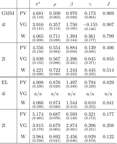
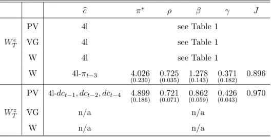
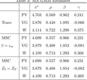
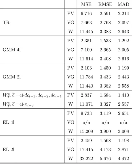
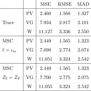
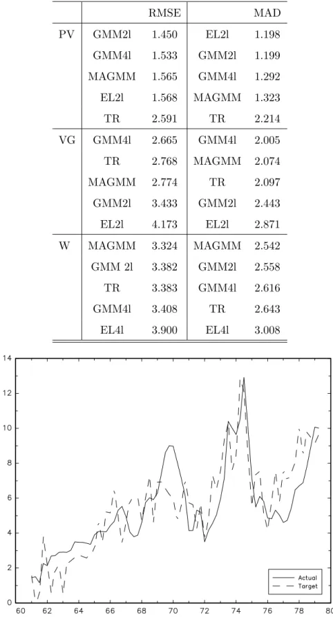
In this section, we estimate the CGG forward-looking monetary policy reaction function for the same period as theirs by GMM and extend the analysis to the GEL and model averaging approaches. The relative merits of each approach are evaluated by building error measures of the di¤erences between the actual and the targeted FED funds rate during the last four decades of the twentieth century.
6.1 A Monetary Policy Rule
We apply the MA GMM approach to the CGG benchmark model. Recall that for any AR lag
p and in‡ation and output delays kand q; the CGG model is given by
it= 1it 1+:::+ pit p+ (1 ) [ + Et t;k+ Etxt;q] +et; (138)
where = i : We adopt their baseline speci…cation for which k = q = 1 (one period
forward) and where the monetary authorities set an expected interest rate that is a linear combination of the target rate and the observed rate at the two previous periods,p= 219 :
it= 1it 1+ 2it 2+ (1 ) [ + Et t+1+ Etxt+1] +et: (139)
Moreover, we take their baseline in‡ation and "output gap" measures. These are the (annualized) rate of change of the GDP de‡ator between two subsequent quarters and the series constructed 1 9CGG also consider the more realistic cases ofk= 4andq= 1and ofk= 4andq= 2but concluded that the