Worcester Polytechnic Institute
Digital WPI
Masters Theses (All Theses, All Years) Electronic Theses and Dissertations
2006-05-03
Association Rule Based Classification
Senthil Kumar Palanisamy
Worcester Polytechnic Institute
Follow this and additional works at:https://digitalcommons.wpi.edu/etd-theses
This thesis is brought to you for free and open access byDigital WPI. It has been accepted for inclusion in Masters Theses (All Theses, All Years) by an authorized administrator of Digital WPI. For more information, please [email protected].
Repository Citation
Palanisamy, Senthil Kumar, "Association Rule Based Classification" (2006).Masters Theses (All Theses, All Years). 661.
Association Rule Based Classification
by
Senthil K. Palanisamy
A Thesis
Submitted to the Faculty
of the
WORCESTER POLYTECHNIC INSTITUTE
In partial fulfillment of the requirements for the
Degree of Master of Science
in
Computer Science
May 2006
APPROVED:
Professor Carolina Ruiz, Thesis Advisor
Professor Matthew Ward, Thesis Reader
Abstract
In this thesis, we focused on the construction of classification models based on association rules. Although association rules have been predominantly used for data exploration and description, the interest in using them for prediction has rapidly increased in the data mining community. In order to mine only rules that can be used for classification, we modified the well known association rule mining algo-rithm Apriori to handle user-defined input constraints. We considered constraints that require the presence/absence of particular items, or that limit the number of items, in the antecedents and/or the consequents of the rules. We developed a char-acterization of those itemsets that will potentially form rules that satisfy the given constraints. This characterization allows us to prune during itemset construction itemsets such that neither they nor any of their supersets will form valid rules. This improves the time performance of itemset construction. Using this charac-terization, we implemented a classification system based on association rules and compared the performance of several model construction methods, including CBA, and several model deployment modes to make predictions. Although the data min-ing community has dealt only with the classification of smin-ingle-valued attributes, there are several domains in which the classification target is set-valued. Hence, we enhanced our classification system with a novel approach to handle the prediction of set-valued class attributes. Since the traditional classification accuracy measure is inappropriate in this context, we developed an evaluation method for set-valued classification based on the E-Measure. Furthermore, we enhanced our algorithm by not relying on the typical support/confidence framework, and instead mining for the best possible rules above a user-defined minimum confidence and within a desired
range for the number of rules. This avoids long mining times that might produce large collections of rules with low predictive power. For this purpose, we developed a heuristic function to determine an initial minimum support and then adjusted it using a binary search strategy until a number of rules within the given range was obtained. We implemented all of our techniques described above in WEKA, an open source suite of machine learning algorithms. We used several datasets from the UCI Machine Learning Repository to test and evaluate our techniques.
Acknowledgement
I would like to thank Prof. Carolina Ruiz for her guidance and encouragement in completing the thesis. This would not have been possible if not for her belief in me. I am also grateful to Prof. Matthew Ward for his comments in shaping the thesis. I would also like to thank fellow students of Knowledge Discovery and Data Mining Group (KDDRG) at WPI for their insights and advice when I needed. I cannot thank enough my wife, Elisabeth, for all her support and encouragement in completing this work. Finally, I would like to dedicate this work to my parents who have been there all along to support me.
Contents
1 Introduction 1
1.1 Overview . . . 1
1.2 Problem Statement . . . 4
2 Background and Related Work 6 2.1 Association Rules . . . 6
2.1.1 Problem Description . . . 7
2.1.2 Apriori Algorithm . . . 7
2.2 Classification . . . 9
2.2.1 Classifier Performance . . . 11
2.3 Classification Association Rules . . . 13
2.4 Other Classifiers . . . 14
2.4.1 Zero-R . . . 14
2.4.2 J4.8 . . . 14
2.5 The WEKA System . . . 14
3 Classification of Single-Valued Class Attributes 17 3.1 Classification based on Association Rules (CBA) . . . 17
3.2 Post Pruning Classification Association Rules . . . 20
3.3.1 Generating Classification Association Rules . . . 22
3.3.2 Generating Rules with Semantic Constraints . . . 22
3.3.3 Classification Models . . . 28
3.3.4 Single Rule and Multiple Rules Classification . . . 30
3.4 Implementation . . . 32
3.5 Experimental Evaluation . . . 38
3.5.1 Evaluation Metrics . . . 38
3.5.2 Experimental Results . . . 40
4 Adaptive Minimum Support 45 4.1 Adaptive Minimum Support . . . 45
4.2 Approach . . . 46
4.3 Initial MinSupport Selection . . . 47
4.4 Adaptive Minimal Support Algorithm . . . 48
4.5 Experiments . . . 50
4.5.1 Experiment Design . . . 50
4.5.2 Summary . . . 52
5 Classification of Multi-Valued Attributes 53 5.1 Association Rule Mining with Set-Valued Attributes . . . 53
5.2 Classification with Set-Valued Class Attribute . . . 54
5.2.1 Set-Valued Class Prediction . . . 54
5.2.2 E-Measure . . . 54
5.2.3 Building Classification Models . . . 56
5.2.4 Model Prediction . . . 58
5.3 Experimental Evaluation . . . 60
5.4 Further Experiments . . . 64
6 Conclusions and Future work 66
6.1 Itemset Pruning . . . 66
6.2 Classification Models . . . 67
6.2.1 Single-Valued . . . 67
6.2.2 Set-Valued . . . 68
List of Figures
2.1 Generation of candidate itemsets and frequent itemsets from the
dataset in Table 2.1 when support count is 3 . . . 10
2.2 Generated rules from frequent itemsets with confidence greater than or equal to 50% . . . 11
3.1 Architecture of WPI Classification System . . . 33
3.2 Parameter Menu For Associative Classification . . . 34
3.3 Parameter Menu for Our Extended Association Rule Mining . . . 39
4.1 Sample Run . . . 52
List of Tables
2.1 Subset of the contact-lenses data set . . . 8
3.1 Attribute-values renumbered to give lower numbers to required at-tributes . . . 23 3.2 Candidate itemsets in the second level of itemset generation . . . 26 3.3 Candidates itemsets in the third level of itemset generation . . . 27 3.4 Generated itemsets and their support in the third level of itemset
generation . . . 27 3.5 Dataset Properties . . . 41 3.6 Experimental Parameters . . . 41 3.7 Comparison of Constraint-based Pruning vs. Non-Pruning for
Mush-room Dataset . . . 41 3.8 Comparison of Constraint-based Pruning vs. Non-Pruning for
Census-Income Dataset . . . 42 3.9 Comparison of Constraint-based Pruning vs. Non-Pruning for
Forest-Cover Dataset . . . 42 3.10 CBA, ARM, J48 and Zero-R on Sonar Dataset (minsupp = 1%,
min-Conf = 50%) . . . 43 3.11 CBA, ARM, Zero-R and J48 on Census-Income Dataset (minsupp =
3.12 CBA, ARM, J48 and Zero-R on Mushroom Dataset (minsupp = 1%,
minConf = 50%) . . . 44
3.13 CBA, ARM, J48 and Zero-R on Forest Cover Dataset (minsupp = 1%, minConf = 50%) . . . 44
4.1 Dataset Properties . . . 51
4.2 Comparison of binary vs linear minSupport strategies in autos dataset 51 4.3 Comparison of binary vs linear minSupport strategies in mushroom dataset . . . 52
5.1 Classifier Model. C stands for confidence and S stands for support . . 58
5.2 Instance whose classification will be predicted . . . 59
5.3 Experimental Parameters . . . 60
5.4 Properties of Movie Dataset . . . 61
5.5 Adaptive Classification-CBA over the Movie Dataset . . . 63
5.6 Adaptive Classification-AR over the Movie Dataset . . . 63
5.7 Non-Adaptive Classification using CBA and AR over the Movie Dataset 64 5.8 Set-Valued Based Classification of Motifs . . . 65
Chapter 1
Introduction
1.1
Overview
Knowledge Discovery and Data Mining (KDD) is playing an important role in ex-tracting knowledge in this era of data overflow. KDD consists of many methods and techniques that can be applied to different data to extract knowledge. Some of the methods include association, classification, and clustering. In this work, we primarily focus on association and classification.
Association rule mining is the discovery of association relationships among a set of items in a dataset. Association rule mining has become an important data mining technique due to the descriptive and easily understandable nature of the rules. Al-though association rule mining was introduced to extract associations from market basket data [AIS93], it has proved useful in many other domains (e.g. microarray data analysis, recommender systems, and network intrusion detection). In the do-main of market basket analysis, data consists of transactions where each is a set of items purchased by a customer. A common way of measuring the usefulness of association rules is to use the support-confidence framework introduced by [AIS93].
Support of a rule is the percentage of transactions that carry all the items in the rule, and the confidence is the percentage of the transactions that carry all the items in the rule among those transactions that carry the items in the antecedent of the rule.
The problem of association rule mining can be stated as: Given a dataset of transactions, a threshold support (minsupport), and a threshold confidence ( min-confidence); Generate all association rules from the set of transactions that have support greater than or equal to minsupport and confidence greater than or equal to minconfidence.
Classification is another method of data mining. Classification can be defined as learning a function that maps (classifies) a data instance into one of several predefined class labels [Mit97]. The data from which a classification function or model is learned is known as the training set. A separate testing set is used to test the classifying ability of the learned model or function. Examples of classification models include decision trees, Bayesian models, and neural nets. When classification models are constructed from rules, often they are represented as a decision list (a list of rules where the order of rules corresponds to the significance of the rules). Classification rules are of the form P → c, where P is a pattern in the training data and c is a predefined class label (target).
As part of this thesis, we study and compare different ways of building models or classifiers from association rules. Given that association rules are descriptive in nature, they are useful in learning about relationships in the data. The learned relationships can be helpful in analyzing the domain. But usefulness of the rules can be further extended if predictive models can be extracted from the rules. Given that the number of rules produced is a function of the minsupport and the minconfidence thresholds, the challenge is to generate an appropriate number of rules that can be
useful in developing predictive models.
Association rule based classification is introduced in [LHM98]. They propose an Apriori like algorithm called CBA-RG for generating rules and another algorithm called CBA-CB for building the classifier. The rules generated by CBA-RG are called classification association rules (CARs), as they have a predefined class label or target. From the generated CARs, a subset is selected based on the heuristic criterion that the subset of rules can classify the training set accurately.
Many other classification systems have been built based on association rules [ZAC02] and [YLW01]. In our work, we have implemented an association rule-based classifier system in the WEKA [FW00] framework. WEKA is a data mining sys-tem developed at the University of Waikato and has become very popular among the academic community working on data mining. We have chosen to develop this system in WEKA as we realize the usefulness of having such a classifier in the WEKA environment. To generate classification association rules, we make use of the AprioriSetsAndSequences algorithm [Pra04] with some optimizations. Apri-oriSetsAndSequences is an extended version of the Apriori algorithm that is capable of mining associations from set-valued and temporal datasets. We have optimized the AprioriSetsAndSequences algorithm to generate only itemsets that can poten-tially yield classification rules that we desire (with the class label as the consequent). More generally, we have adapted the algorithm to generate only rules that satisfy user specified constraints. We achieve this by integrating these constraints into the mining phase so that we can use the constraints to prune itemsets that would not yield rules of the type that the user desires.
We have also extended our classification system to handle set-valued classes. To the best of our knowledge, the problem of multi-class classification has not been studied in the association rule mining domain. We evaluate our system with gene
expression data and compare our results with previous projects which have used this application domain.
In many cases, the number of rules produced by an association rule mining system is either too low or too high to be useful. Therefore, a goal of this thesis is to experiment with techniques to limit the cardinality of the set of association rules to predefined ranges. We hope to achieve this by using an adaptive minimum support approach [LAR02], where the support is modified based on the cardinality of the set of association rules, until the cardinality matches the predefined range.
1.2
Problem Statement
The overall goal of this thesis is to design and develop a classification system that is based on Association Rule Mining in the WEKA environment. Our problem can be further broken down as follows:
• Adapt the Apriori algorithm to generate classification association rules (CARs) efficiently.
• Build Classification Models.
– Build a framework to generate models from CARs.
– Provide different modes for deploying a model in order to classify novel instances.
– Extend the framework to handle set-valued class attributes.
• Implement an adaptive scheme that searches for an optimal minimum support threshold allowing the user to specify only the desired range of rules and the minimum confidence threshold.
As part of our extensions to the classification system to handle set-valued class labels, we propose and discuss two different methods for predicting set-valued at-tributes. In this regard, we use the notions of E-measure [LG94] and F-measure [LG94] from information theory to compare the predicted set attribute with the actual set attribute.
Chapter 2
Background and Related Work
In this chapter, we introduce association rules, classification, and integrated asso-ciative classification. Also, we look at different existing classification systems built upon association rule mining systems.
2.1
Association Rules
Association rule mining was introduced in [AIS93] as a way to find associative pat-terns from market basket data. The market basket data consist of transactions where a transaction is a set of items purchased by a customer. The motivation for applying this data mining approach on market basket data was to learn about buying patterns and use that information in catalog design, and store layout design. Since then, association rule mining has been studied and applied in many other domains (e.g. credit card fraud, network intrusion detection, genetic data analysis). In every domain, there is a need to analyze data to identify patterns associating different attributes. Association rule mining addresses this need.
Many association rule mining algorithms have been proposed in the data mining literature. Apriori [AS94] and FP-growth [HPY00] are two of them. Apriori uses
the property, all nonempty subsets of an frequent itemset must also be frequent [AS94] to prune the search space. Apriori follows a breadth-first-search strategy while FP-growth follows a depth-first search strategy. Several extensions of the basic association rule mining algorithm have been published. One of them is the CBA-RG algorithm [LHM98], which adapts Apriori to generate classification association rules efficiently. The generated rules are used in CBA-CB [LHM98] to extract a classification model. We have implemented CBA-CB as part of our model building system. Other extensions to Apriori include mining rules with constraints [SVA97a].
2.1.1
Problem Description
The general problem of association rule mining is: Given a data set of transac-tions where each transaction is a set of items, a minimum support threshold and a minimum confidence threshold, find all the rules in the data set that satisfy the specified support and confidence thresholds. Let I be a set of items, D be a data set containing transactions (i.e, sets of items in I) and t be a transaction. An association rule mined from D will be of a form X → Y, where X, Y ⊂ I and X ∩Y = ∅. The support of the rule is the percentage of transactions in D that contain both X and Y. The confidence is, out of all the transactions that contain X, the percentage that contain Y as well. Confidence of a rule can be computed as support{X∪Y} ÷support{X}. The confidence of a rule measures the strength of the rule (correlation between the antecedent and the consequent) while the support measures the frequency of the antecedent and the consequent together.
2.1.2
Apriori Algorithm
The Apriori algorithm was introduced in [AS94] as a way to generate association rules from market basket data. The Apriori algorithm is a two stage process: A
frequent itemset (itemsets that satisfy minimum support threshold) mining stage and a rule generation stage (rules that satisfy minimum confidence threshold).
In Table 2.1, we show a subset of the contact-lenses data set from the University of California Irvine (UCI) Machine Learning Repository [KPSB00]. We will generate association rules from this data set (Figure 2.1).
age astigmatism tear-prod-rate contact-lenses
young no normal soft
young yes reduced none
young yes normal hard
pre-presbyopic no reduced none
pre-presbyopic no normal soft
pre-presbyopic yes normal hard
pre-presbyopic yes normal none
presbyopic no reduced none
presbyopic no normal none
presbyopic yes reduced none
presbyopic yes normal hard
Table 2.1: Subset of the contact-lenses data set
Each attribute-value pair is referred to as an item. For brevity, attribute-value pairs are denoted only by their values. For example, age = young will be written as young.
2.1.2.1 The Frequent Itemset Mining Stage
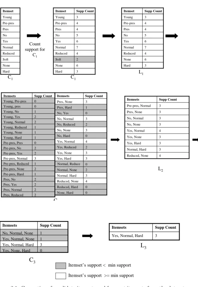
In the first iteration of Apriori’s frequent itemset mining stage, each item becomes part of the 1-item candidate set C1. The algorithm makes a pass over the data set to count support for C1, see Figure 2.1. Those itemsets satisfying the minimum support will form L1, the set of frequent itemsets of size 1. The ones that have support less than the minimum support threshold are shown in gray in Figure 2.1.
To generate candidates of size 2 (C2) itemsets, the level 1 collection of frequent itemsets is joined with itself. This join is denoted by L1 on L1 and is equal to the
collection of all set unions of different itemsets in L1. The algorithm scans the database for support of the items in C2. Those itemsets satisfying the minimum support condition will form L2.
When generating candidates of size 3 (C3), L2 on L2 is performed but with a condition. Apriori assumes that the items in an itemset are sorted according to a predefined order (e.g. lexicographic order). The join, Lk on Lk for k > 1, has the
condition that for two itemsets from Lk to be joined, the first k−1 item(s) must
be the same in both itemsets. This ensures that the generated candidate is of size k and that most of the subsets of the set are frequent. Before counting support for all the items in C3, the Apriori property is applied. The Apriori property [AS94] states that all nonempty subsets of an itemset must be frequent for this itemset to be frequent. The Apriori property prunes the search space.
The Apriori algorithm continues to generate frequent itemsets until it cannot generate any more candidate itemsets.
2.1.2.2 The Rule Generation Stage
The frequent itemsets produced are used to generate association rules that satisfy minimum support and minimum confidence. For each frequent itemset, all possible splits of the itemset into two part (antecedent and consequent) are generated and the rule so generated is outputted by the Apriori if the rule satisfies the minimum confidence condition as seen in Figure 2.2.
2.2
Classification
Classification is the process of learning a function or a model from a data set (training data) so that the function can be used to predict the classification of a novel instance,
Itemset Hard None Soft Reduced Normal Yes No Pres Pre-pres Young Supp Count Itemset 3 Hard 6 None 2 Soft 4 Reduced 7 Normal 6 Yes 5 No 4 Pres 4 Pre-pres 3 Young Supp Count Itemset 3 Hard 6 None 4 Reduced 7 Normal 6 Yes 5 No 4 Pres 4 Pre-pres 3 Young C1 C1 Count support for C1 L1 1 Pre-pres, Hard 1 Young, Reduced 1 Young, None 1 Young, Hard 2 Young, Normal 0 Young, pres 1 Young, No 2 Young, Yes 0 Young, Pre-pres 2 Pres, Reduced 2 Pres, Normal 2 Pres, Yes Supp Count Itemsets 2 Pres, No 2 Pre-pres, None 1 Pre-pres, Reduced 3 Pre-pres, Normal 2 Pre-pres, Yes 2 Pre-pres, No 0 Pre-pres, Pres Supp Count Itemsets 0 None, Hard 0 Reduced, Hard 4 Reduced, None 3 Normal. Hard 2 Normal, None 0 Normal, Reduce 3 Yes, Hard 3 Yes, None 2 Yes, Reduced 4 Yes, Normal 0 No, Hard 3 No, None 2 No, Reduced 3 No, Normal 0 No, Yes 1 Pres, Hard 3 Pres, None C2 L2 4 Reduced, None 3 Normal, Hard 3 Yes, Hard 3 Yes, None 4 Yes, Normal 3 No, None 3 No, Normal 3 Pres, None 3 Pre-pres, Normal Supp Count Itemsets 0 Yes, None, Hard
3 Yes, Normal, Hard
1 Yes, Normal, None
1 No, Normal, None
Supp Count Itemsets
C
3Itemset’s support < min support Itemset’s support >= min support
3 Yes, Normal, Hard
Supp Count Itemsets
L
3Figure 2.1: Generation of candidate itemsets and frequent itemsets from the dataset in Table 2.1 when support count is 3 10
Tear-prod-rate = reduced contact-lenses = none [ Conf: 1.0, Sup: 0.36] Contact-lenses = none tear-prod-rate = reduced [Conf: 0.67, Sup: 0.36 ] Astigmatism = yes tear-prod-rate = normal [ Conf: 0.67, Sup: 0.36] Tear-prod-rate = normal astigmatism = yes [ Conf: 0.57, Sup: 0.36]
Figure 2.2: Generated rules from frequent itemsets with confidence greater than or equal to 50%
whose classification is unknown. Classification models are frequently represented as rules of this form: P → c where P is a pattern in the training data (P forms the set of predicting attribute(s)) and c is the class label or target attribute.
Some of the common classification techniques are decision trees, na¨ıve Bayes, and neural nets [HPY00]. In this thesis, we will study the building of classification models or classifiers from association rules.
2.2.1
Classifier Performance
Classifier performance is usually measured by accuracy, the percentage of correct predictions over the total number of predictions made. Many other measures are also used to understand the different aspects of the generated model such as: sensitivity, specificity precision and recall [HPY00]. In this thesis, we will primarily focus on precision and recall, which are measures borrowed from information retrieval. These measures are defined as follows:
precision = true positives
true positives + false positives
recall = true positives
To understand true/false positives and negatives, let us use an example from information retrieval. One common example would be a web search engine returning results based on a user query. Let us define Q as the query. For any given Q, the answer space, G, can be split into what is relevant and what is not relevant. The returned answerAmay contain some relevant information and/or some non-relevant information. Among the results A, the relevant information is called true positives, and the non-relevant information is called false positives. Among results that are not returned (G-A), the relevant information forQis called false negatives and the non-relevant information is called true negatives. So precision is a ratio of relevant results to all results and recall is a ratio of relevant results to all relevant information. The initial phase of the process is model(classifier) construction. A model is defined as a function that can map an unlabeled instance to a predefined class label. A model is constructed from data where each instance has a class label. These data are called the training set. The constructed model is tested to determine how well it predicts new instances. Testing can be done in different ways: test over the training set or test over an independent test set. Testing the classifier over the training set is usually not a good way to measure the accuracy of the classifier since the classifier has been constructed from the same data. But the testing on the training set is useful in identifying any errors in model construction. A poor accuracy rate on the training set may mean a poorly learned classifier. Using a separate test set is a good way of determining how well the classifier will perform on novel instances.
Training and testing can be accomplished in different ways depending on the amount of available data. If the number of instances available is large, the available data set may be split into a training set and a testing set (usually 66% for training and the rest of testing is considered a good split). This method of training is often a luxury in many domains as the data available for training may be insufficient.
The number of training instances has a direct effect on the classifying ability of the model built from that number of instances. When there is a limited amount of data for training and testing, n fold cross-validation is a preferred way to maximize the use of available data to produce a good classifier. Innfold cross-validation, the data is divided inton folds, and each fold in turn is used for testing, while the other folds are used for training. The reported accuracy is the average over the n iterations of training and testing.
2.3
Classification Association Rules
The use of association rules for classification was proposed in [LHM98]. In as-sociative classification, the focus is to produce association rules that have only a particular attribute in the consequent. These association rules produced are called class association rules(CARs).
Associative classification differs from general association rule mining by introduc-ing a constraint as to the attribute that must appear on the consequent of the rule. The produced rules can be used to build a model or classifier. CARs are a particular case of constrained association rules. There has been research in this area about integrating (pushing) these constraints into the mining phase rather than filtering the enormous number of rules produced using the constraints as post-processing filters. One paper on this area [SVA97b] proposes different ways of pushing the constraints into the mining phase. The general advantages are faster execution and lower memory utilization.
The CBA-RG algorithm is an extension of the Apriori algorithm. The goal of this algorithm is to find all rule items of the form < condset, y >wherecondsetis a set of items, and y∈Y where Y is the set of class labels. The support count of the
rule item is the number of instances in the data set D that contain the condset and are labeled with y. Each rule item corresponds to a rule of the form: condset→y. Rule items that have support greater than or equal to minsup are called fre-quent rule items, while the others are called infrefre-quent rule items. For all rule items that have the same condset, the one with the highest confidence is selected as the representative of those rule items. The confidence of rule items are calculated to determine if the rule item meets minconf. The set of rules that is selected af-ter checking for support and confidence is called the classification association rules (CARs).
2.4
Other Classifiers
2.4.1
Zero-R
Zero-R is a very basic classification technique that predicts the majority class from the training set and is useful as a benchmark to compare performances of other classifiers [FW00]. In the case of numeric attributes, Zero-R predicts the average value of the target attribute from the training set.
2.4.2
J4.8
J4.8 is Weka’s [FW00] implementation of the C4.5 decision tree algorithm [Qui93].
2.5
The WEKA System
The Waikato Environment for machine learning, Weka, [FW00] is an open source machine learning environment with many useful data mining and machine learning
algorithms. Currently, Weka is the de-facto machine learning and data mining envi-ronment at Worcester Polytechnic Institute (WPI). Members of the WPI Knowledge Discovery and Data mining Research Group (KDDRG) have modified algorithms as well as embedded their work into the Weka environment. One such work includes merging the Apriori implementation in Weka with the Apriori implementation in another data mining system called ARMiner [SS02]. This work has improved the working of the association rule mining part in terms of speed and memory utilization. The ARMiner system was adapted earlier by Shoemaker [Sho01] to generate asso-ciation rules from set-valued datasets. The merged algorithm is called AprioriSets [SS02].
AprioriSets was further modified to handle sequence type data [Pra04]. The new algorithm is known as AprioriSetsAndSequences [Pra04]. Algorithm 1 outlines Weka’s procedure for generating association rules. The input parameters include minimum confidence, upperBoundMinSupport, lowerBoundMinSupport, delta, and minNumberOfRules. The upperBoundMinSupport and the lowerBoundMinSupport form the support range within which the algorithm tries to satisfy the minNum-berOfRules required. The delta parameter is the value by which the support gets lowered each time the Apriori algorithm is repeated. Initially, support is set to upperBoundMinSupport and if the number of rules generated does not satisfy the minNumberOfRules, the support is reduced by delta and the process is repeated until either the number of rules generated satisfies the minNumberOfRules or the support becomes smaller than the lowerBoundMinSupport. In Step 5, the 1-item itemsets are generated (refer to Section 2.1.2 for the working of Apriori algorithm). In steps 6-10, candidates and frequent itemsets of size starting two are generated until no more candidates can be generated. In step 11, maximum frequent itemsets, that is frequent itemsets that have no frequent supersets, are generated from the
frequent itemsets. In step 12, all possible rules are generated satisfying the min-Confidence condition. If the number of rules produced is greater than or equal to minNumberOfRules or if the minSupport is lower than the lowerBoundMinSupport, the while loop is broken and the rules are returned.
In the AprioriSetsAndSequences algorithm, each attribute-value pair is repre-sented by an integer. A mapping of the numbers to the attribute-value pair is stored in a hash table. Before the rules are generated, each number is replaced by its corresponding attribute-value pair.
Algorithm 1 Weka’s Procedure for Generating Association Rules
Inputs: UpperBoundMinSupport, LowerBoundMinSupport, delta, minNumberOfRules, minConfidence
Output: rules
1. rules = ∅;
2. freqItemsets =∅;
3. support = UpperBoundSupport;
4. while (support ≥LowerBoundSupport AND rules.size <minNumberOfRules) do 5. L1 ={1-item itemsets}; 6. for (k = 2;Lk−16=∅)do 7. Ck = generateCandidates(Lk−1); 8. Lk = evaluateCandidates(Ck); 9. freqItemsets ∪ L(k); 10. end for 11. maxFreqItemsets = genMaxFreqItemset(freqItemsets);
12. rules = GenerateAllRules(maxFreqItemsets, minConfidence);
13. support = support - delta;
14. freqItemsets =∅;
15. end while 16. return rules;
Chapter 3
Classification of Single-Valued
Class Attributes
3.1
Classification based on Association Rules (CBA)
In this chapter, we focus on generating association rules for building classification models. The chapter consists of our proposed modifications to an association rule mining algorithm to generate classification rules. The generated rules are used to build a classification model, which is evaluated with different prediction modes to study its predictive capability.
The rules resulting from Associative Classification mining can be evaluated to select a subset of the rules that will form the model or classifier. To the best of our knowledge, Liu, Hsu, and Ma [LHM98] were the first to produce a classifier based on association rules. They show that the classifier built performs as well as or better than well known decision tree algorithms. Since then, many association rule based classifiers have been built for various domains. Among others, [ZAC02] for classifying mammography images, [YLW01] for classifying web documents, [LAR02]
for recommender systems, [CAM04] for classifying spatial data, [YL05] for document classification, and [CYZH05] for text categorization. The process of building the classifier involves selecting rules by confidence or support. Confidence is a popular criterion for rule selection to the classifier as it denotes the strength of a rule. In the case of CBA [LHM98], they use a heuristic to select a subset of the rules that classifies the training set most accurately. In some cases, the pruning is as simple as removing contradicting rules [ZAC02] or more complicated like using post pruning techniques that are used in decision trees [YLW01].
In CBA-CB [LHM98], the generated CARs are ordered based on the following definition.
Definition 3.1. Rule Ordering () Association Given two rules, ri and rj, ri rj (ri precedes rj) if • the confidence of ri is greater than that of rj or,
• their confidence are the same, but the support of ri is greater than that of rj,
or,
• both the confidence and the support ofri andrj are the same, butri is generated
earlier than rj.
LetRbe the set of CARs andDbe the training data. The aim of the model con-struction algorithm is to choose a set of highly predictive rules inRto cover the train-ing dataD. The classifier built is of the following form: < r1, r2, ..., rn,default class>
where ri ∈R, ra rb if a < b. Default class is the default label used when none of
the rules can classify an instance.
Algorithm 2 shows the CBA-CB procedure[LHM98]. In step 1, the rules are sorted according to the order mentioned above; then each rule is considered in turn.
Algorithm 2 CBA-CB Algorithm
Inputs: rules R, training set instances D Output: classifier C
1. R = sort(R);
2. for each rule r∈R in sequence do 3. temp=∅
4. for each instanced∈D do
5. if d satisfies the conditions of r then
6. store d.id intemp and mark r if it correctly classifies d;
7. end if
8. end for
9. if r is marked then 10. insert r at the end of C;
11. delete all the cases with the ids in temp from D;
12. select the default class for the current C;
13. compute the total number of errors of C;
14. end if
15. end for
16. Find the first rule p in C such that Cp, the list of rules in C up to p, has the lowest
total number of errors. and drop all the rules.
17. Add the default class associated with p to the end of C, and return C
The rule under consideration is marked if it can classify at least one instance in the training set correctly (steps 5 and 6). If the rule is marked, all the instances covered by the rule are removed from the training set and the majority class of the rest of the training instances becomes the default class label (steps 11 and 12). The marked rule is added to the end of the classifier.
Let Cr denote the lists of rules ending in rule r that have been selected for
inclusion in the classifier so far. In step 13, the classifier Cr is used to classify the
instances of the training set, and evaluate the performance of the classifier. Since the classification values of the instances are known, each classification attempt or prediction can be recorded as a correct classification or wrong classification. When all the instances are classified, the classifier will be assigned an error rate which is the total number of wrong classifications over the total number of classifications.
added after this rule are removed. The default class label attached with that rule becomes the default class label of the classifier (step 17).
3.2
Post Pruning Classification Association Rules
With association rule mining, the number of rules produced might be overwhelming. As all the produced rules may not be interesting or significant, it is important to prune those rules deemed uninteresting or overfitting (rules that are very specific to the training set). Similar to decision tree post-pruning, association rules can be post-pruned to reduce the number of rules produced. Many ideas on post-pruning of decision trees were introduced by Quinlan [Qui93]. There are basically two ap-proaches to post-pruning based on error rates [FW00]. One is to divide the data set into training, validation and testing sets. With this approach, the rules will be built using the training set, and pruning will be done based on the performance of the rules on the validation set. With the second approach, there is no separate validation set, but the training set is used as the validation set. The latter technique is known as pessimistic error pruning.
Pessimistic error pruning is a heuristic based on statistical reasoning [Qui93] (see also [FW00]). For each rule, let the number of errors on the training set be E and the number of cases covered on the training set be N (those instances containing the antecedent of the rule). The observed error rate is f=E/N. Let the true error rate (unknown) beq. Here, we assume the N instances are generated by a Bernoulli process with probability q and error rate E.
The mean and variance of a single Bernoulli trial with success ratep are p and p(1−p) respectively. ForN Bernoulli trials, the success ratef is a random variable with mean equal to p, and the variance is reduced to p(1−p)÷N. For large N, the
value of the random variable f approaches a normal distribution.
The probability that a random variable,X, with 0 mean lies within a confidence range of width 2z is
P r[−z ≤X ≤+z] =c
where c is the confidence level.
For random variablef to have a 0 mean and unit variance, we subtract mean p from f and divide by standard deviation σ, where σ=p
p(1−p)/N. P r " f −q p q(1−q)/N > z # =c
The upper confidence limit for q in the expression above provides a pessimistic estimate of e (see [FW00]) error rate at a given node:
e= f + z2 2N +z q f N − f2 N + z2 4N2 1 + z2 N
Rule R is compared with its subrules, that is rules in which one or more items are removed from the antecedent of R. If a rule R has a higher pessimistic error rate than any of its subrules, R is pruned while retaining the subrules.
3.3
Association Rule Based Classification Model
Construction
In this section, we describe the approach we have taken to accomplish our primary goal of building a classification system based on association rules. This includes generating classification rules from AprioriSetsAndSequences and carrying out post-pruning to reduce the cardinality of the set of generated rules and building models from the pruned rules.
3.3.1
Generating Classification Association Rules
As we mentioned in the Chapter 2, classification association rules (CARs) are a subset of association rules with a predefined target or class in the consequent. An inefficient way of obtaining CARs is to generate all the frequent itemsets for a data set and in the process of generating rules from these itemsets, prune away rules that do not conform to CARs.
In our work, we have generated only those frequent itemsets that can produce CARs while the others are pruned away at the frequent itemset mining phase. Every CAR has a class attribute or target on the consequent of the rule. As this target is predefined, we can use this target as a semantic constraint to generate frequent itemsets consisting of the class attribute.
Definition 3.2. Semantic Constraints
A semantic constraint is a requirement that an attribute(s) must appear or must not appear in the antecedent and/or consequent of a rule.
Definition 3.3. Syntactic Constraints
A Syntactic constraint is a requirement placed on the number of attribute-value pairs on either the antecedent or consequent of a rule.
3.3.2
Generating Rules with Semantic Constraints
In many cases, we are interested in generating rules with one or more semantic constraints. In the contact-lenses data set depicted in Table 2.1, we may want to generate rules such that the contacts, age and tear prod rate are represented in each of them. These three attributes contribute to the semantic constraints. For the rules to have these three attributes, the frequent itemsets must contain them. Therefore, it will suffice if we generate only items sets that include the three attributes we
are interested in. The frequent itemset may have other attributes. We are able to use the semantic constraints as conditions in the join step of the Apriori candidate generation phase.
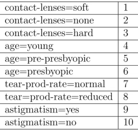
The approach we have used to prune itemsets that do not contain the required attributes is closely related to the implementation of AprioriSetsAndSequences. Our goal is to generate only itemsets that have all the required attributes (constraints). In the AprioriSetsAndSequences algorithm [Pra04], each attribute value pair is mapped to a number (item number), see Section 2.5. This numbering is done in such a way that the attribute values of the first attribute in the data set receives the lowest numbers followed by the attribute values of the second attribute and so on. A hash table stores the mapping between the numbers and the attribute values. Numbers assigned to an attribute’s values are consecutive.
To allow for pruning of itemsets that may not contain the attributes we desire, we reorder the attributes so that the attributes that are semantic constraints (required attributes) are given smaller numbers than the non-required attributes. Therefore, in the contact-lenses data set, attribute-values of contacts, age, and tear prod rate will be assigned smaller numbers than the values of the other attribute, astigmatism, as show in Table 3.1. contact-lenses=soft 1 contact-lenses=none 2 contact-lenses=hard 3 age=young 4 age=pre-presbyopic 5 age=presbyopic 6 tear-prod-rate=normal 7 tear=prod-rate=reduced 8 astigmatism=yes 9 astigmatism=no 10
Definition 3.4. Sorted Set of Semantic Constraints
Let A = {a1, a2, ..., an} be the set of attributes in the data set. A sorted set C = {c1, c2...ck} is defined as the set of semantic constraints such that ci ∈ A for all
i, 1 ≤ i ≤ k, and constraints are sorted such that ci precedes ck if i < k and
a1 =c1, a2 =c2. . . ak =ck.
Modified Itemset Generation Join Step
A candidate itemset of size (k + 1) is generated from 2 itemsets X and Y of size k where X precedes Y in lexicographic order if the following two conditions are satisfied:
• if X containsm constraints wherem >1, the constraints must be the first m constraints from the set of constraints (i.e., c1, c2, . . .cm).
• ifX contains less thankconstraints, it cannot contain a non-constrained item.
Theorem 3.1. Let A={a1, a2, . . . , an} be the set of attributes in the data set. Let
C = {c1, c2, . . . , ck} be the set of semantic constraints such that ci ∈ A for all i,
1 ≤ i ≤ k. Let X and Y be two itemsets such that X ≤ Y and a1 = c1, a2 = c2. . . ak =ck. If itemsets X and Y do not satisfy the the following conditions then
the join of X and Y cannot generate a rule that satisfies all the constraints in C. • if X contains m constraints where m > 1, the constraints must be the first m
constraints from the set of constraints (i.e., c1, c2, . . ., cm).
• ifX contains less thank constraints, it cannot contain a non-required attribute (non-constrained attribute).
Proof. We reiterate that the attribute-value pairs will be ordered such that those that are required attributes(constrained attributes) will be placed lower than the
non-required attributes in the lexicographic order. In the join step, we can make a determination as to whether the join of X and Y will produce an itemset that has the potential to end up with all the required attributes.
Given X ={x1, x2, .., xn−1, xn} and Y ={y1, y2, .., yn−1, yn} where x1. . . xn and
y1. . . yn are items representing attribute-value pairs. For X and Y to join, the
apriori join condition, x1 =y1, x2 =y2, xn−1 =yn−1 and xn6=yn must be true. The join of X and Y will result in an itemset of size n+ 1.
The first condition we have introduced as part of theorem 3.1 is that ifX con-tains items fromm constraints, those m constraints must be the firstm constraints based on lexicographic order. Otherwise, Xwill join with aY that does not have the constraint. Let us suppose that X does not contain an item from cj where j ≤m.
As we know that X will join with Y such that the first n−1 items from both X and Y are the same, which means Y will also not contain an item from cj. The
resulting itemset Z of size n+ 1 will not contain cj. Using the previous argument,
we know that Z cannot join with another itemset such that the missing constraint cj can be included in the resulting set. This shows that any itemsets resulting from
the original X will not have cj and therefore neither X nor any of its supersets will
form rules that satisfy all the constraints.
The other condition we have introduced as part of theorem 3.1 is that the X cannot contain item(s) from non-required attributes as long as it does not contain all the required attributes. Let us consider the different cases that X can take in terms of having required and non-required attributes:
Case 1: If itemsetX contains only items from required attributes while adhering to the first condition mentioned above, i.e., items from 1. . . n are required and are in order. In this case, X can join with Y, such that the X and Y have the same number of items n and the first n−1 items of X and Y are the same. This join
will go ahead as we cannot make a determination as to if this resulting itemset will have all the constraints.
Case 2: If itemsetX contains items some required attributes,c1, c2, cj wherej <
k and one non-required attributeam. In this case,Xcan only join with aY that has
the same set of items from the same set of required attributes,c1, c2, cj with one
non-required attribute. The resulting Z itemset will not become a potential candidate for rule generation as it is missing the required attributes cj+1. . . ck. Therefore, X
will not be joined with Y.
Case 3: If itemset X contains all the required attributes and one non-required attribute. In this case, asX has met the criteria, we can joinXwith the appropriate Y.
3.3.2.1 Generating Frequent Itemsets
Let us generate frequent itemsets from the contact-lenses data set:
In Figure 3.1, we showed the attribute-value pairs and how they are numbered. The required attributes are: contacts, age and tear prod rate.
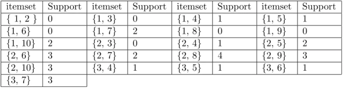
itemset Support itemset Support itemset Support itemset Support
{ 1, 2 } 0 {1, 3} 0 {1, 4} 1 {1, 5} 1 {1, 6} 0 {1, 7} 2 {1, 8} 0 {1, 9} 0 {1, 10} 2 {2, 3} 0 {2, 4} 1 {2, 5} 2 {2, 6} 3 {2, 7} 2 {2, 8} 4 {2, 9} 3 {2, 10} 3 {3, 4} 1 {3, 5} 1 {3, 6} 1 {3, 7} 3
Table 3.2: Candidate itemsets in the second level of itemset generation
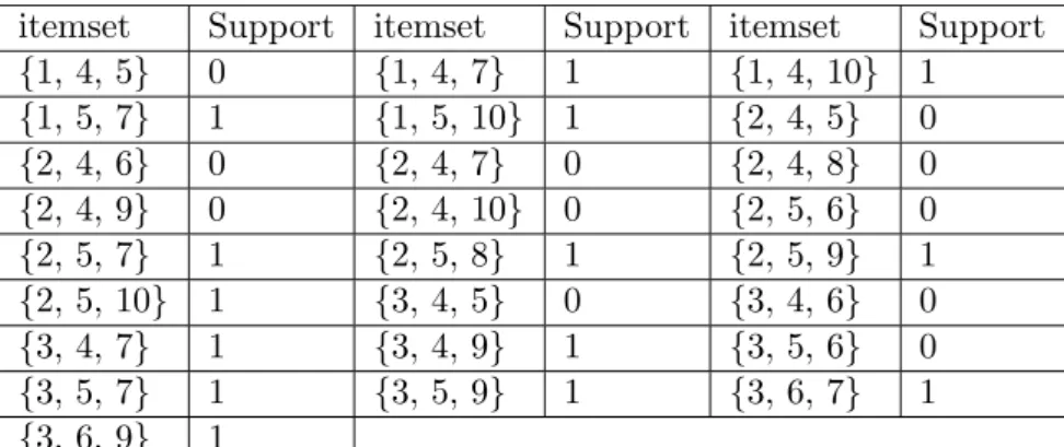
In Tables 3.2, 3.3 and 3.4 we show the candidate itemsets generated and their support until no more candidate itemsets can be generated. We use minimum support as 1, at least one data instance must contain the itemsets for the itemsets to be considered for the next level. Those itemsets with support less than 1 were
itemset Support itemset Support itemset Support {1, 4, 5} 0 {1, 4, 7} 1 {1, 4, 10} 1 {1, 5, 7} 1 {1, 5, 10} 1 {2, 4, 5} 0 {2, 4, 6} 0 {2, 4, 7} 0 {2, 4, 8} 0 {2, 4, 9} 0 {2, 4, 10} 0 {2, 5, 6} 0 {2, 5, 7} 1 {2, 5, 8} 1 {2, 5, 9} 1 {2, 5, 10} 1 {3, 4, 5} 0 {3, 4, 6} 0 {3, 4, 7} 1 {3, 4, 9} 1 {3, 5, 6} 0 {3, 5, 7} 1 {3, 5, 9} 1 {3, 6, 7} 1 {3, 6, 9} 1
Table 3.3: Candidates itemsets in the third level of itemset generation
itemset Support itemset Support itemset Support
{1, 4, 7, 10} 1 {1, 5, 7 , 10} 1 {2, 4, 8, 9} 0
{2, 5, 7, 8} 0 {2, 5, 7, 9} 1 {2, 5, 7, 10} 0
{2, 5, 8, 9} 0 {2, 5, 8 , 10} 1 {3, 4, 7, 9} 1
{3, 5, 7, 9} 1 {3, 6, 7, 9} 1
Table 3.4: Generated itemsets and their support in the third level of itemset gener-ation
dropped from the frequent itemsets group that was used in generating candidate itemsets for the next level.
In Table 3.2, we observe that only itemsets starting with an item from the first attribute, contact-lenses, is generated. This is a result of itemset pruning that is part of itemset generation.
3.3.2.2 Generating Maximal Frequent Itemsets
All the frequent itemsets generated from the itemset generation step are used to generate maximal frequent itemsets. A maximal frequent itemset is an itemset that is not a subset of any other itemset. This stage reduces the number of itemsets we are working with significantly.
3.3.2.3 Counting Support for those Itemsets without Support
Using the maximal itemsets, we generate all the subsets of the maximal itemsets and determine if each subset has support counted. As we know from the item-set generation stage, some itemitem-sets may not be generated because of the itemitem-set pruning step and therefore will not have their support counted. Those itemsets without support will need to have their support counted prior to the rule gener-ation stage. When generating rules from the maximal itemsets, a pruned itemset may appear on the antecedent or consequent of a rule. Suppose X represents the antecedent and Y represents the consequent, confidence of a rule is computed as support{X∪Y} ÷support{X}. Therefore, it is essential that all subsets of a max-imal itemset have their support counted.
3.3.2.4 Generating Classification Association Rules
In the case of generating association rules, all possible splits of a frequent itemset into antecedents and consequents are considered. However, in generating classifica-tion associaclassifica-tion rules, syntactic constraints are placed such that the rule generated has only items from the classification attribute on the consequent side, while no items from the classification attribute are present on the antecedent side. Further, confidence is calculated for each rule and those rules with confidence greater than or equal to the minimum confidence will form the final set of classification association rules.
3.3.3
Classification Models
In the previous sections, we discussed generating constrained classification associ-ation rules (CARs). In this section, we focus on building and using classificassoci-ation
models.
3.3.3.1 Building Classification Models
A classification model is a function that maps a novel unlabeled instance to a prede-fined class. In our work, we consider two types of models, all rules models (where all the produced CARs are used in the model) and the CBA model [LHM98], described in Section 3.1
The CBA algorithm [LHM98] is based on a heuristic and selects a subset of rules that classifies the training set most accurately. The CBA algorithm satisfies the condition that each new instance is predicted by the rule with the highest confidence.
3.3.3.2 Deploying Classification Models
Given a model and a new instance whose class is unknown, the problem of predicting the instance’s class using the model is an interesting problem. There is more than one way to use the model to predict the instance’s class. In association rule based classification models, rules in the model are ordered as follows:
• if rule ri has greater confidence than rj, then ri precedes rj, or
• if ri has the same confidence as rj, then the rule with greater support will
precede the other, or
• if ri has the same support and the same confidence as rj, then the rule with
then smaller number of items in the antecedent will precede, or
• ifri has the same support, confidence and antecedent size asrj, then the order
Rules of high confidence are thought to be good for classification. Confidence alone may not make a rule very good. For instance, a rule from an instance that appears only once (high confidence but low support) may not be a good rule for clas-sification. Rules with very high confidence and low support are useful in identifying rare events.
3.3.4
Single Rule and Multiple Rules Classification
In CBA [LHM98], a single rule is used to classify a new case. Though this may be a simple and logical way to classify, it has been shown to be less effective than using multiple rules [LHP01]. Suppose, we want to determine if a person is eligible for a bank loan with the following attributes (housing = rent, employ status = yes, income ≥50K). Imagine we have a model to classify a new case as eligible for loan or ineligible for loan. If the top three rules that match this case are as follows:
• housing = rent → loan = NO (Sup:0.01, Conf:1.0)
• income ≥50K → loan = YES (Sup:0.05, Conf:0.93)
• employ status = yes → loan = YES (Sup:0.15, Conf:0.9)
If we use just one rule to classify as in CBA[LHM98], we would classify the new case as loan = NO. If we consider all the three rules together, we would classify the new case as loan = YES. This shows that the class label assigned will depend on the modes of classification and it is important to have both the modes available to be able to compare and contrast the accuracies resulting from the two modes.
The following sample model will be used to explain the different ways of predict-ing an unknown subject or case. Let us assume our model consists of three rules in the following order:
1. age=young −→ contact-lenses=none [Sup:0.05, Conf: 0.9]
2. age=young AND tear-prod-rate=normal −→ contact-lenses=none [Sup:0.03, Conf: 0.8]
3. age=young AND astigmatism=no−→contact-lenses=none [Sup:0.02, Conf:0.78]
4. age=young AND astigmatism=yes−→contact-lenses=soft [Sup:0.015, Conf:0.75]
Let us consider the data instance: age = young AND tear-prod-rate=normal AND astigmatism=yes and assume that we want to predict the class label for this instance, that is, if the user requires a contact-lenses and if so what type.
3.3.4.1 Single Rule Prediction
All the rules are sorted by confidence and then by support. The class associated with the first rule that covers the instance is selected as the prediction.
If we have to use the above mentioned model to predict the contact-lenses type for a young individual, we will select the first rule (has the highest confidence) and the prediction is that contact-lenses are not prescribed.
3.3.4.2 Prediction by Weighted Majority
All rules that cover the new instance are selected and confidence (or support) is used to weigh the predictions made by each of these rules. The majority of this weighted prediction is selected as the model’s prediction.
In this mode, we will use confidence to select the appropriate class label. Rules 1, 2 and 4 can be used to predict the contact-lenses type. We will use confidence as the weight to select which class is appropriate. The weight of each prediction is calculated by summing up the confidence values for different classifications from the rules which cover the new instance:
P
ConfRclass = 1.70 where class=none
The weight of the new instance being soft is: P
ConfRclass = 0.75 where class=sof t
We select the class label with the highest weight and contact-lenses=none is predicted as the class label for the test instance.
3.4
Implementation
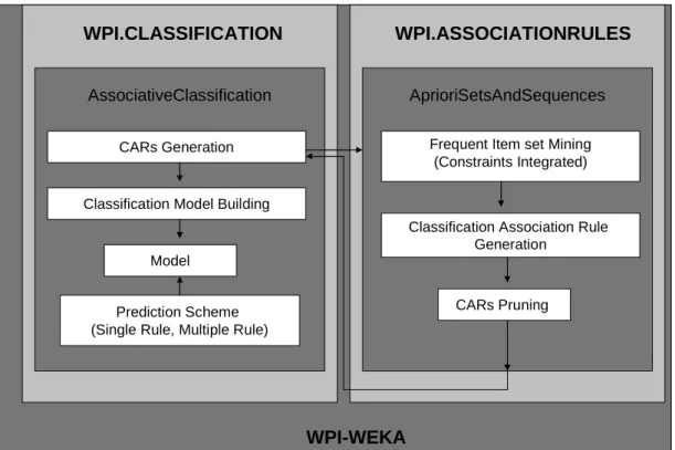
We have implemented our classification system in WEKA [FW00]. WEKA is an open-source suite of machine learning algorithms. The motivation for implement-ing our thesis in WEKA is the extensive use of this system in WPI’s Knowledge Discovery and Data Mining Research Group. WEKA is developed in the Java Pro-gramming Language. Figure 3.1 shows the architecture of our classification system. We modified the existing Apriori like algorithm, AprioriSetsAndSequences [Pra04] (see Section 2.5), to generate classification association rules. The generated rules are used for building models. The resulting models are tested for accuracy.
WPI.CLASSIFICATION
AssociativeClassification
CARs Generation
Classification Model Building
Model
Prediction Scheme (Single Rule, Multiple Rule)
WPI.ASSOCIATIONRULES
AprioriSetsAndSequences
Frequent Item set Mining (Constraints Integrated)
Classification Association Rule Generation
CARs Pruning
WPI-WEKA
Figure 3.1: Architecture of WPI Classification System
Referring to Figure 3.1, the association rule based classification algorithm is called AssociativeClassification and is part of the Wpi.Classifiers package. We show the interaction between AssociativeClassification and AprioriSetsAndSequences. We also show the different modules in both the algorithms.
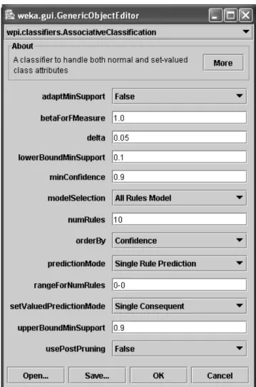
Figure 3.2: Parameter Menu For Associative Classification
Figure 3.2 shows the parameter menu for AssociativeClassification. In this menu, the user can specify the following options: minimum confidence, minimum support, starting support, support delta, minimum number of rules, which model to build (CBA or All Rules Model), if post-pruning is allowed, and how to pre-dict (single rule or multiple rule). The new parameters added by our work include: modelSelection, predictionMode and usePostPruning. For description of other pa-rameters, please see Chapter 2.
• modelSelection - the type of algorithm used to select a classification model
(e.g., CBA, All Rules Model)
• predictionMode - which prediction method to follow (e.g., Single Rule, Multi-ple Rules)
• usePostPruning - whether to post prune the association rules based on pes-simistic error before building a classification model. See Section 3.2
Algorithm 3 is the modified control procedure to mine (constrained) CARS. In this thesis, we have modified the original control procedure (see Algorithm 1) to allow pruning of rules based on pessimistic error. We have also modified the algorithm to allow for presence or absence of items (semantic constraints) in the rules. More precisely, users can specify an item to appear or not to appear on either the antecedent or the consequent of a rule. We use a pruning technique to generate only itemsets that can potentially become part of the user specified rules. In the rule generation step, before a rule is generated, it is checked to see if it satisfies the user specified constraints and, if so, the rule gets generated. WEKA contains many well known classification algorithms and one significant contribution of this thesis is the classifier based on Association rule mining algorithm.
Input parameters include requiredAntecedent, requiredConsequent, disallowedAn-tecedent and disallowedConsequent. The while loop in Step 5 repeats itself until the support threshold is below the minsupport or the number of rules generated suffices according to the user specified number of rules. If we look into the iterative process of generating itemsets and rules from them: In Step 6, we generate the 1-item itemsets. In steps 11-15, the condition exhausts all possible itemsets that can be produced until no more items of size k can be joined to produce items of size (k+1). Only those itemsets that will potentially yield rules with the required itemsets are generated. The algorithm for this can be seen in Section 3.3. The
Algorithm 3 Modified AprioriSetsAndSequences Control Procedure
Inputs: requiredAntecedents, requiredConsequents, disallowedAntecedents, disallowedCon-sequents, numRules
Outputs: rules
1. rules = ∅;
2. support = UpperBoundSupport;
3. freqItemsets =∅;
4. requiredItems = requiredAntecedents ∪ requiredConsequents
5. while (support >minsupport AND rules.size <numRules) do 6. L1 ={1-item itemsets}; 7. for (k = 2;Lk−16=∅)do 8. Ck = generateCandidates(Lk−1, requiredItems); 9. Lk = evaluateCandidates(Ck); 10. freqItemsets ∪ L(k); 11. end for 12. maxFreqItemsets = genMaxFreqItemset(freqItemsets);
13. rules = GenerateAllRules(maxFreqItemsets, requiredAntecedents, requiredConse-quents);
14. rules = PruneRules(rules);
15. if (rules.size > minRules)then 16. return rules;
17. end if
18. support = support - delta;
19. end while
generated candidates are evaluated to see if they have minimum support (step 13). In step 16, the frequent itemsets are used to generate the maximal frequent itemsets. In 17, we generate all rules according to user requests on required antecedents and consequents. In step 18, the rules may be pruned if the pruning option is set on. If the resulting number of rules is equal to or exceeds the user desired number of rules, the rules are returned.
Algorithm 4 is the AssociativeClassification algorithm that we have developed as the core of our classification system. In step 1, the input parameters are passed to AprioriSetsAndSequences algorithm to generate classification rules. Using the user specified model parameters, a model is generated from the classification rules. In step 4, the model is tested against the test set and the results are shown on the screen.
Algorithm 4 AssociativeClassification
Inputs: minrules, minimum confidence, minimum support, starting support, rule post-pruning (boolean), model, prediction, trainingSet
Output: modelTestResults
1. rules = AprioriSetsAndSequences(trainingSet, numRules, minSupport, startingSup-port, minConf, numRules);
2. rules = sort(rules);
3. model = generateModel(rules, model);
4. testModel(model);
5. outputStats();
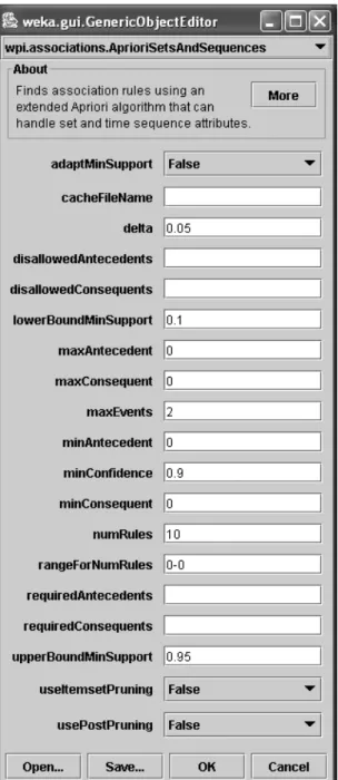
Figure 3.3 shows the parameter menu for association rule mining. In this thesis, we included the following parameters:
• disallowedAntecedents - those attributes not to appear on the left hand side of the rules.
• disallowedConsequents - those attributes not to appear on the right hand side of the rules.
• adaptMinSupport - switch to use adaptive minimum support (see Chapter 5).
• numRules - applies in the case when adaptive minimum support is used.
• useItemSetPruning - switch to use itemset pruning in the mining stage based on required antecedents and consequents or do not prune itemsets.
• usePostPruning - switch to use post pruning based on pessimistic error to reduce the number of generated rules.
• maxEvents - AprioriSetsAndSequences is capable of handling set-valued and sequential data. See [Pra04] for details on this and other sequence related parameters.
3.5
Experimental Evaluation
In this section, we describe the experiments carried out to compare and evaluate our classification system. We break down this section into data description, evaluation metrics and experimental results. We show the performance improvement obtained by pushing pruning of itemsets at the frequent itemset generation level and the models built by the classifier with different experimental settings.
3.5.1
Evaluation Metrics
We evaluate the classifier based on error rate with different prediction schemes. We also report the accuracy rate. The error rate signifies the number of wrong predictions over the total number of predictions. The accuracy rate signifies the number of correct predictions over the total number of predictions.
accuracy = number of correct classifications total number of classifications made
error= number of incorrect classifications total number of classifications made
A prediction involves selecting an appropriate class label for a case whose class label is unknown. For example, let < x1, x2, ... xk, ? > be a data instance whose class
label is unknown (denoted by a question mark). xi represents the value of attribute
i of the instance. If this data instance is given as an input to a model, the rule(s) that covers this instance (the features of the rule are a subset of the features in the data instance) will determine the class label for the data instance.
3.5.2
Experimental Results
We divide this section into two parts. In part 1, we focus on the improvements made to AprioriSetsAndSequences by itemset pruning in the presence of constraints. Here we evaluate performance based on time taken for mining and generating rules and the number of maximal frequent itemsets generated. A frequent itemset is considered maximally frequent if none of its supersets is frequent.
3.5.2.1 Data Set
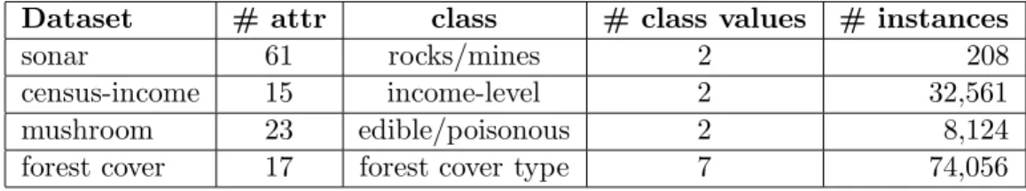
We tested the classification system with the following datasets obtained from the UCI Machine Learning Repository [SHM98]: census-income, mushroom and forest cover. Table 3.5 shows the properties of these datasets. As part of pre-processing, continuous valued attributes were discretized using WEKA’s instance based dis-cretization filter with the number of bins set to 10 [FW00].
Dataset # attr class # class values # instances
sonar 61 rocks/mines 2 208
census-income 15 income-level 2 32,561
mushroom 23 edible/poisonous 2 8,124
forest cover 17 forest cover type 7 74,056
Table 3.5: Dataset Properties
3.5.2.2 Itemset Pruning in the presence of Constraints
As part of our experiments, we were interested in comparing itemset pruning vs. non-pruning. We ran experiments with the mushroom, census-income and forest cover datasets. We generated single and multiple constraint classification rules. We observed the resulting parameters such as the number of itemsets produced, number of maximal itemsets produced and time taken for generating rules.
Table 5.3 shows the parameters used in running the experiments. In these experiments, the goal was to generate as many rules as possible with the support greater than or equal to 1%. The minimum confidence was set to 50%.
Support Confidence
1% 50%
Table 3.6: Experimental Parameters
Prune Req. Ant Req. Con itemsets Rules Max. itemsets Time(s)
No none class 45391 21101 158 4951
Yes none class 42620 21101 42 4357
No odor class 45391 8288 158 1153
Yes odor class 33160 8288 26 1813
Table 3.7: Comparison of Constraint-based Pruning vs. Non-Pruning for Mushroom Dataset
In Table 3.7, we present the results for the mushroom dataset. The first column shows if constraint based pruning was selected or not. In the case of pruning being switched off, all candidate itemsets are used in generating valid itemsets at each level of the Apriori process. In comparing the first two rows (single constraint), we observe
the reduction in the number of itemsets produced and the reduction in time taken for generating the rules. But interestingly, in the next two rows (double constraint) even though the number of itemsets produced decreases, the time taken increases. We figured this is a case where a large number of item-subsets are dropped from consideration due to the constraint based pruning. The final scan of the database for support of those items costs a significant time, increasing the overall time (see Section 3.3.2.3).
Prune Req. Ant Req. Con itemsets Rules Max. itemsets Time(s)
No none class 1071 350 82 85
Yes none class 410 350 36 88
No relationship class 1071 22 82 87
Yes relationship class 100 22 31 16
Table 3.8: Comparison of Constraint-based Pruning vs. Non-Pruning for Census-Income Dataset
As seen in Table 3.8, in the case of a single constraint, the results for pruning and non-pruning are very similar. In the case of two constraints, the pruning leads to better performance in terms of time, approximately 1/5 of the time taken without pruning.
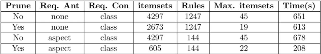
Prune Req. Ant Req. Con itemsets Rules Max. itemsets Time(s)
No none class 4297 1247 45 651
Yes none class 2673 1247 19 613
No aspect class 4297 144 45 678
Yes aspect class 605 144 22 208
Table 3.9: Comparison of Constraint-based Pruning vs. Non-Pruning for Forest-Cover Dataset
In Table 3.9, we observe reduction in time with pruning in both single constraint and double constraint.
3.5.2.3 Comparison of Different Classifiers
In this set of experiments, we compared the performance of the CBA classifier with the All Rules Model (ARM) classifier. We also compared these performances with other well-known classifiers such as Zero-R and J-4.8 (Decision Trees). In the case of CBA and ARM, we also experimented with the different prediction modes such as Single Rule and Weighted by Confidence. In these experiments, we used a split of 66% for the training set and the rest for the testing set.
Classifier Pred Mode Test Option Accuracy Num Rules
CBA Single Rule 66% split 74.65% 44
CBA Weight(conf) 66% split 73.42% 44
ARM Single Rule 66% split 76.05% 33733
ARM Weight(conf) 66% split 64.78% 33733
Zero-R - 66% split 54.93% 1
J4.8 - 66% split 70.43% 11
Table 3.10: CBA, ARM, J48 and Zero-R on Sonar Dataset (minsupp = 1%, minConf = 50%)
Table 3.10 shows the results for the sonar dataset using CBA, ARM and other classifiers. Both CBA and ARM perform better than J48, Prism and Zero-R. In fact, ARM produces the best accuracy of 76.05% with single rule prediction. In the case of CBA, the best accuracy is obtained with Single Rule prediction mode of 74.65%.
Classifier Pred Mode % Split Accuracy Num Rules
CBA Single Rule 66% 83.5% 545
CBA Weight(conf) 66% 83.5% 545
ARM Single rule 66% 80.87% 9754
ARM Weight(conf) 66% 80.87% 9754
J4.8 66% 84.07% 331
Zero-R 66% 76.27% 1
Table 3.11: CBA, ARM, Zero-R and J48 on Census-Income Dataset (minsupp = 1%, minConf = 50%)
Table 3.11 shows the results for CBA, ARM and other classifiers with the cen-sus income data. In this case, J4.8 performs marginally better than CBA. ARM performs below CBA in both modes. In the case of CBA, both modes perform similarly.
Classifier Pred Mode % Split Accuracy Num Rules
C