Estimating portfolio value at risk by a conditional copula approach in BRICS countries

(1)

COPYRIGHT AND CITATION CONSIDERATIONS FOR THIS THESIS/ DISSERTATION

o Attribution — You must give appropriate credit, provide a link to the license, and indicate if changes were made. You may do so in any reasonable manner, but not in any way that suggests the licensor endorses you or your use.

o NonCommercial — You may not use the material for commercial purposes.

o ShareAlike — If you remix, transform, or build upon the material, you must distribute your contributions under the same license as the original.

How to cite this thesis

Surname, Initial(s). (2012). Title of the thesis or dissertation (Doctoral Thesis / Master’s Dissertation). Johannesburg: University of Johannesburg. Available from:

(2)

ESTIMATING PORTFOLIO VALUE AT RISK BY A CONDITIONAL COPULA APPROACH IN BRICS COUNTRIES

by

TSHIKENDA LEOPOLD MUKALENGE

A dissertation submitted in fulfilment for the Degree Of

Master’s in Commerce In Financial Economics

At the

College of Business and Economics

UNIVERSITY OF JOHANNESBURG

Supervisor: Prof Qing- Guo Wang

(3)

i | P a g e

ABSTRACT

This thesis used daily log returns of indices of BRICS countries from the period of March 11th_{2013 to May 16}th_{2017. Its main focus was to estimate the value at risk (VaR) of a}

portfolio of the BRICS financial markets using a conditional copula approach.

A useful starting point was to apply the model of AR (1)-GARCH (1,1) with t-distribution and AR (1)-GARCH (1,1), using returns of the normal errors for the marginal distribution models in the copula framework. Two copulas, the normal and the symmetric Joe Clayton (SJC) copulas, were estimated as both constant and varying. The log likelihood of the time-varying copula was significantly more suitable than the constant copula.

The comparison of the performance of the copula models to the benchmark AR (1)-GARCH (1,1) was done using the Christoffersen test. The 99% VaR appeared fairly accurate, suggesting that the VaR models were dependable. The standard level of comparison AR (1)-GARCH (1,1) did not perform well compared to the SJC copula; i.e. the time-varying SJC copula performed better than the benchmark model. The time-varying SJC copula model used to estimate the portfolio VaR also showed a minimum number of exceptions in the back-test. This copula thus meets regulatory capital requirement for investors as stipulated in Basel II.

(4)

ii | P a g e

ACKNOWLEDGEMENTS

Firstly, I would like to take this opportunity to convey my appreciation and gratitude to my supervisor, Dr. Wang Qing-Guo, for his valuable guidance and encouragement during this thesis . The resources and advice that he provided were indispensable and I am grateful for the helpful pointers and clarifications he provided. Without his input, completing this mini-dissertation would not have been possible.

Special thanks go to my wife, Samba Kayembe Celestine, and the family Tshikenda. It is very difficult to express in words my gratitude for all sacrifices they have made for me.

Lastly, I wish to extend my deepest gratitude to the Baha i Community, and to all my friends, especially Leon Mishindo, Olivier Musampa and Dr Alain Mwamba, who supported me in many ways during the period of study.

(5)

iii | P a g e

LIST OF FIGURES

Figure 5-1: The complete data set of the price indices of all stock markets ... 23

Figure 5-2: The log returns series of original data ... 24

Figure 5-3: QQ-plots of the returns of the stock market indices versus normal density ... 28

Figure 5-4: Plot of JSE and SENSEX ... 29

Figure 5-5: Plot of JSE and MICEX ... 30

Figure 5-6:Figure 6: Plot of JSE and IBOV... 30

Figure 5-7: Plot of JSE and SSE ... 31

Figure 5-8: The dependency structure: Normal and SJC copulas – upper and lower tail dependence between the South African and Indian stock markets (JSE-SENSEX) ... 43

Figure 5-9: Constant and time-varying normal copula and SJC copulas – upper and lower tail dependence between South African and Brazilian stock markets (JSE-IBOV) ... 44

Figure 5-10: Constant and conditional normal copula and the SJC copulas – lower and upper tail dependence between South African and Russian stock markets (JSE-MICEX) ... 45

Figure 5-11: The dependency structure of normal copula and the SJC copulas – lower and upper tail dependence between South African and Chinese stock markets (JSE-SSE) ... 46

(8)

vi | P a g e

LIST OF TABLES

Table 5-1: ADF and PP unit root test results ... 25

Table 5-2:Descriptive statistics of daily returns stock indices *... 26

Table 5-3: Linear correlation between the five returns of BRICS indices ... 29

Table 5-4: Results for AR (1)-GARCH (1,1) – Normal estimations ... 33

Table 5-5: Represents the estimation of AR (1)-GARCH (1,1) – student t ... 34

Table 5-6: P-value for standardized squared residuals and standardized residuals ... 36

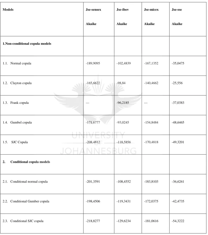
Table 5-7: Comparison copula models (AIC) ... 37

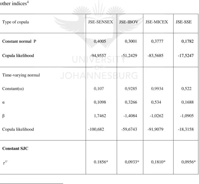
Table 5-8: Dependence of estimated parameters of copulas between the South Africa index and other indices ... 38

Table 5-9: Summary statistics of the time-varying correlation variable ... 41

Table 5-10:Summary statistics of the measure of tail dependence ... 42

Table 5-11:Back-testing results for the pair JSE-SENSEX ... 48

Table 5-12:Back-testing results for the pair JSE-IBOV ... 48

Table 5-13: Back-testing tests results for the pair JSE-MICEX ... 49

Table 5-14: Back-testing tests results for the pair JSE-SSE ... 49

Table 5-15:Comparative analysis for Latin-American, Europe and North America, and BRICS 50

(9)

vii | P a g e

LIST OF SYMBOLS

ADF Augmented Dickey-Fuller test

ARCH Autoregressive conditional hesteroscedasticity

ARMA Autoregressive moving average

BRICS Brazil, Russia, India, China, South Africa

BSE Bombay Stock Exchange

CDF Cumulative distribution function

DAX Deutscher Aktien Index

EVT Extreme Value Theory

EWMA Exponential Weighted Mean Average

FTSE FTSE 100 Index

GARCH The generalized autoregressive conditional heteroscedasticity

IBOV Bolsa de Valores do Estado de Sao Paulo

JSE Johannesburg Stock Exchange

LR Likelihood ratio

MICEX Moscow Interbank Currency Exchange

MLE Maximum likelihood estimation

PP Phillips-Peron test

SENSEX Sensitive Index

SJC Symmetrized Joe-Clayton

SSE Shanghai Stock Exchange

TSX Toronto Stock Exchange

(10)

1 | P a g e

Chapter: I Introduction

1.1 Background and problem statement

In financial institutions such as investment firms and banks, risk management is of great importance. Indeed, Basel II (Basel Committee on Banking Supervision, 2011) requires financial institutions to provide minimum financial capital to cover potential losses related to their exposure toward credit risk, operational risk and market risk. It is recommended that these institutions use value at risk (VaR) to measure the specific portfolios in terms of market risks. VaR is considered to be the worst loss over a given confidence level and time horizon.

During the last few years, risk management has become a critical concern in financial industry. In order to estimate and regulate market, credit and operational risks, final institutions put in developing reliable risk measurement and management techniques.

The use of Value at Risk models is among the main advanced technique. These models help to evaluate the worst expected loss of portfolio of financial instrument at a pre-specified time and level confidence. One of the attractive property is to summarize market risks in one single number. This simple outcome is very significant for risk managers because it makes this technique very informative and easily understood.

The weakness of the VaR models is related to its dependence on distributional assumptions. Besides this weakness, risk managers have emphasized in the idea of adding VaR estimates the stress testing technique.

Risk management is characterized by the volatility forecasts of the portfolio return. Therefore, a firm needs a time dynamic forecast that will take into account the dynamic properties of variance such as volatility clustering. Good forecasting also provides better control of market financial risks and lead to good decisions.

VaR is a single, summary, statistical measure of possible portfolio losses aggregates all of the risk. Specifically, value at risk is a measure of losses due to normal market movement. Losses greater than the value at risk are suffered only with a specified small probability. Subject to the simplifying assumptions used in its calculation, value at risk aggregates all of the risks in a portfolio into a single number suitable for use in the board room, reporting to regulators, or disclosure in an annual report, one crosses the hurdle of using a statistical measure, the concept

(11)

2 | P a g e of value at risk is straight forward to understand. It is simply a way to describe the magnitude of the likely losses on the portfolio.

The two most important characteristics of VaR are: the availability of risk across different positions and risk factors. It enables us to measure the risk associated with a fixed-income position risk. VaR give us a common risk yardstick, and this measure makes it possible for institutions to manage their risks in new ways. VaR models take account for the correlation is essential if we are to able to handle portfolio risks in a statistically meaningful way.

1.2 Objective of thesis

The use of the multivariate conditional distribution, specifically in terms of the asymmetric dependence and heavy tails, is crucial to the application of financial methods such as portfolio selection, asset pricing, and risk management and forecasting. However, research thus far has generally concentrated on developed markets. Few studies have examined the role of South Africa in the global economy, particularly as emerging economy. This current dissertation follows on previous research and attempts to estimate the VaR of a portfolio formed from the major stock indices in the BRICS countries using the copula framework.

The focus here will be mostly on South Africa’s dependence on the BRICS countries. A time-varying conditional copula as suggested by Patton (2006) will be used, thus the normal and the SJC copulas will be used, both with and without time-varying parameters and marginal distribution for the GARCH innovations.

In risk management, VaR thus plays a central role. At present, quantification of the asset market risk or a portfolio VaR has become the standard risk measurement applied by financial analysts. Three approaches are considered for estimating the VaR of portfolio: the historical simulation, variance-covariance (also called analytical variance) and Monte Carlo simulation approaches. However, Sollis (2009) states that variance-covariance approach (used in the risk metrics model) underestimates VaR owing to its assumption of distribution, the historical approach can be altered in same size and the Monte Carlo simulation approach may suffer through an incorrect assumption of distribution.

Moreover, the most important element in estimating VaR is the distribution of the financial logarithms returns of the assets constituting the portfolio. This process assumes that the logs of asset returns follow a normal distribution. However, this assumption has not verified when the

(12)

3 | P a g e distributions of financial log returns series have large tails and are leptokurtic. Consequently, VaR models based on this approach tend to undervalue the risk.

Since the release of the risk metrics methodology, the analytical process has been generally used. Because the analytical process accepts the theory of the joint distribution of the assets returns by multivariate normal law, the best measure of risk is the variance, and the usual measure of dependence between the assets is the covariance matrix. However, as indicated above, this assumption of normality is not often adequate in finance.

The procedure used to determine VaR is thus critical. In financial, actuarial and economics studies, modelling with copulas has been used widely for multiple applications. The copula theory was initially presented as a means to separate the dependence structure among distribution functions. Applying copula theory risk analysis has also been discussed in finance literature, with most current studies generally using copulas in the context of developed countries, and only a few considering emerging markets.

An important study is that of Patton (2002) who has modelled time-varying conditional dependence in a recent extension to the conditional case of copula theory. In an earlier study, Patton (2001) used a proposition initially presented by Sklar (1959). This proposition establishes that an k-dimensional distribution function might be separated into its copula and k-marginal distributions. Note that copula expresses the dependence between the n variables. Patton has also extended Sklar’s theorem to conditional probabilities, and has applied this theorem to the modelling of time-varying joint probabilities of the Yen exchange rate and Deutsche mark returns.

Palaro & Hotta (2006) presented some concepts and properties of the copula function and showed how the conditional copula theory can be a very powerful instrument to simulate the portfolio VaR with constituent NASDAQ and S&P500 indices. They used different copulas and marginal distribution for GARCH innovation and compared the results obtained with traditional methods of VaR estimation. They found that the symmetrized Joe-Clayton (SJC) copula allows for different dependences in the tail, producing the best results and reliable VaR limits.

Van der Houwen (2014) then later applied the parameters of the constant and time-varying SJC and normal copulas to the AR (p)-GARCH (1, 1) model of the returns of equity price indices of the DAX-FTSE 100, S&P500-FTSE 100 and S&P500-S&P/TSX. Applying a likelihood

(13)

4 | P a g e ratio test, he found that the conditional copula provided a considerably better model fit than the copula with constant parameters.

1.3 Methodology

We have chosen the copula framework to estimate the VaR of a portfolio built upon the main stock market indices of BRICS countries. The objective of the thesis is to assess the performance of copula methodology with respect to those of the parametric AR (1,0)-GARCH (1,1) model. The benchmark model will be AR (1,0)-GARCH (1,1).

1.4 Relevance of thesis

The VaR model is one of the most common tools for estimating market risk, as it can offer information about the loss of a portfolio with an assumed confidence level. In turn, the estimation of the dependence of the time-varying conditional correlations model between variables is crucial in the construction of both a portfolio and its VaR (Embrechts et al., 2005). Because investors nowadays have more financial products from which to choose, the VaR evaluation of a portfolio is becoming more and more important. A risk manager concerned about likely loss might choose the lower tail of a copula, whereas a portfolio manager might choose the dependence structure of copula. This thesis provides valuables tools to policy makers, financial agents, and investors dealing with estimation of portfolio VaR using a conditional copula.

1.5 Structure of the thesis

The thesis is structured around six chapters. The introduction presented above is Chapter 1, and is followed by the literature review in Chapter 2. Chapter 3 addresses the BRICS markets, while Chapter 4 displays the econometric techniques used in the study, namely copulas, GARCH models and VaR and back-testing. Chapter 5 then illustrates the data and displays the econometric estimation, which is centred on the application of the conditional copula to estimate the portfolio VaR of the major indices in BRICS countries. Chapter 6 is the conclusion, and offers concluding remarks.

(14)

5 | P a g e

Chapter 2 Literature review

Various studies have discussed the methods and approaches for modelling VaR of diverse financial markets, and modelling with copulas specifically has been widely used for multiple applications in actuarial, economic and financial studies. This section reviews both the empirical and theoretical studies that have been conducted about VaR and copula models and relates their findings to this current study.

Copula theory was introduced over sixty years ago as a means to isolate the dependence structure among distribution functions. Partial solutions were first advanced by Hoedfing, (1940), Fretchet (1951) and Dall’Aglio (1956) among distribution functions. Sklar (1959) then consolidated those advances, creating a new class of distributions whose margins are uniform in (0, 1).

Sklar (1959) introduced the idea and the name of copula and, as such, the respective theorem now bears his name –, Sklar’s theorem. From Dowd (2005) point of view, the power of the copula resides in the fact that it does not rely on assumptions related to joint distribution with regards to the financial assets of portfolio. Indeed, in finance, the hypothesis of normality is not suitable, as shown in Patton (2006) and (Ang & Chen, 2002). In their empirical study, these authors established a large correlation among asset returns during unstable markets and markets slumps. This deviation from normality indicates the inadequacy of the VaR measurement. As a risk measurement technique in financial markets, the copula has thus been considered a valuable tool. It has been used in option valuation by McNeil et al. (2015) to investigate the period structures of the interest rates by Junker et al. (2006), in credit risk analysis by Giesecke (2004) and Cherubini et al. (2004) and to estimate the operational risk in banking by Demoulin et al. (2006)

Two VaR estimation models for six currencies have been presented by Nguyen & Huynh (2015), in which every series of return is supposed to follow an ARCH (1,1)-GARCH (1,1) model, and innovations are simultaneously produced using t-distributions and Gaussian copulas. Bob (2013) estimated VaR for a portfolio including Germany, Spain, France and Italy, combining copula functions, extreme value theory, and GARH models. In an earlier study based on semi-parametric approaches and using copula-extreme value, Hsu et al. (2012)

(15)

6 | P a g e assessed portfolio risk for six Asian markets. In the simulation of VaR as suggested by Monte Carlo, they show that the Joe-Clayton copula EVT yields the best results concerning the shapes of the return distributions. Also using the Monte Carlo approach, Rank (2007) demonstrated the reliability of copula methodology for VaR analysis. He applied copula theory to create various scenarios of VaR.

Torres & Olarte (2009) also employed copula modelling for VaR analysis, while Embrechts et al. (2005) used copula methodology to create diverse scenarios for VaR analysis. In 2011, Shim et al. (2011) applied a copula approach to measure economic capital, VaR and expected shortfall. In their attempt to optimize portfolios, Krzemienowski & Szymczyk (2016) applied a copula based on extension of conditional VaR, while Yingying et al. (2016) examined the risk contagion and correlations among mixed assets and mixed-asset portfolio VaR measurements. Their approach followed a dynamic view based on time-varying copula models. It should be noted that most studies are based in developed financial markets; copula studies on emerging markets are still scarce. Some early studies include research by Hotta, et al. (2008) and Ozun & Cifter (2011), who applied copula theory in VaR valuation in Latin American emerging market portfolios.

However, the methodology of the copula used in early research does not have a variable characteristic over time. In other words, this methodology does not include conditionality, and is what Rosengerg (2003) calls a constant copula. Patton (2002) developed the conditional copula through the variation in time between the first and the second conditional moments. The technique is now considered to be a VaR estimation.

A few years later, Rockinger & Jondeau (2006) demonstrated the challenges that the model of the dependence between stock market returns encounters when it follows a complicated dynamic fluctuation. In the case where the distributions are non-normal, it is not easy to precisely identify the multivariate distribution linking two or more return series. As such, they proposed a new method grounded on copula functions, which contains the approximation of the joint distribution and the univariate distributions. The dependence parameter can simply be extracted in both conditional and time-varying copulas. Their results suggested conditional dependency depending on past realizations for pairs of European markets only. Dependency, for these markets, is influenced more when returns move in the same direction than when they move in opposite directions. These authors also show in the modelling of dynamics of the dependency parameter that dependency is higher and more persistent in the middle of European

(16)

7 | P a g e stock markets. Chen & Fan (2006) also utilized the copula structure to build a semi-parametric model based on the Markov approach.

Rockinger and Jondeau (2001) investigated a parametric copula conditional to the position of past joint observations in the unit square, combined with preceding marginal estimation of GARCH-type models with time-varying kurtosis and skewness. They considered the S&P500 and the Nikkei 225 for the return European stock indices and applied Hansen’s generalized student’s t as the error distribution for the GARCH models and the Plackett’s copula. Their results provide empirical evidence that the dependency between financial returns may change through time.

Applying the copula and the historical empirical distribution in the estimation of marginal distributions, Cherubini and Luciano (2001) estimated the VaR. They employed the copula as another possibility for the multivariate GARCH models. Lee and Long (2005) then combined the multivariate GARCH model with the copula, allowing the flexibility of the joint distributions to evaluate the VaR of a portfolio composed of S&P500 and NASDAQ indices. They proposed, with uncorrelated dependent errors, a copula-multivariate GARCH model as compared with three multivariate GARCH models, and proved that the empirical mixed-model performs well as a multivariate GARCH in terms of in-sample model choice criteria and an out-sample multivariate density forecast.

In considering the above, it is evident that research using copula for estimating VaR has been conducted over the past ten years. However, most of these studies are based on developed countries, with little attention paid to emerging countries. Moreover, in the first investigations, the copula method applied did not contain conditionality – in other words, a time-varying feature. As such, we attempt to analyse the BRICS markets, using the copula method to calculate the VaR of a portfolio composed of their major stock market indices and to consider the performance of copula method compared to the parametric model AR (1,0)-GARCH (1,1). Such a study is necessary, as today stockholders have more financial products from which to choose, and the VaR evaluation of a portfolio is becoming increasingly important. The aim of the thesis is likewise to provide valuable tools to polices makers, financial agents, and investors in terms of using a conditional copula in portfolio VaR estimation.

(17)

8 | P a g e

Chapter: 3 BRICS markets

A stock market index is a measurement of the value of a specific sector of a stock market. It is computed from the price of particular stocks, typically a weighted average, by investors and financial managers in order to describe the market and to assess the returns on specific investments.

3.1 Introduction

An index is a mathematical notion that cannot be invested in directly. However, many exchange-traded funds and mutual funds try to “track” an index, and these funds may be compared to those that do not “track” an index.

When considering the returns of a national stock index, the assumption is that the index portrays the distribution of the particular national stock market. The target stock indices in this thesis include IBOVSPA (Brazil), MICEX (Russia), SENSEX (India), SSE (Chinese) and JSE (South Africa). Each of these indices will be discussed below.

3.2 IBOVSPA Index (Brazil)

The IBOVESPA index represents an index of about 50 stocks traded on the Sao Paulo Stock, Futures Exchange & Mercantile Markets. The index consists of a conjectural portfolio, with the stocks accounting for 80% of the quantity traded in the previous 12 months, and is revised quarterly. he elements of the IBOVESPA about 70% of the entire stock value traded. IBOVESPA is an accumulation index representing the actual value of a portfolio started in 1968 with an initial value of 100 adjusted according to share price increase and adding the reinvestment of all dividends, subscription rights and bonus stocks received.

3.3 MICEX Index (Russia)

One of the major universal stock exchange in East Europe and the Russia Federation is MICEX, or the Moscow Interbank Currency Exchange. As an important Russian stock exchange, MICEX opened in 1992. As of December 2010, approximately 239 Russian companies were listed, with a market capitalization of USD 950 billion. Considering the overall volume traded in the Russian Stock Market, MICEX represents the large majority (more than 90%). In 2011, MICEX merged with Russian Trading System, creating the Moscow Exchange.

(18)

9 | P a g e

3.4 Bombay Stock Exchange - SENSEX (India)

The S&P Bombay Stock Exchange Sensitive Index, also called SENSEX, is a free-float-market-weighted stock market index, constructed on 30 financially sound companies listed and well-established on the Bombay Stock Exchange. These are some of the largest and most actively traded stocks, and are related to various industrial sectors of the India economy. The S&P SENSEX was formed 1978-79, with a value of 100 on 1 April 1979.

Currently, India represents an emerging market with about 8,000 listed stocks. There are two major stock exchange markets – the National Stock Exchange (NSE) and the Bombay Stock Exchange (BSE). Because the BSE is the largest stock market with the most trading activity in India, it was selected for this study. Corporations listed on BSE commanded a total market capitalization of USD 1.68 trillion as of March 2015 (World Federation of Exchanges, 2015).

3.5 The Shanghai Stock Exchange (China)

The Chinese index is a stock market index of all stocks that are traded on the Shanghai Stock Exchange (SSE). The SSE is based in the city of Shanghai, China. Its main characteristic is that the SSE is one of the stock exchanges that operates autonomously in the People’s Republic of China – the other is the Shenzhen Stock Exchange. The SSE is among the largest stock markets in the world. In February 2008, SSE listed 861 companies, and total market capitalization of the SSE reached USD 3, 241.8 billion (USD 1= RMB 6.82).

3.6 FTSE/JSE ALL SHARE Index (South Africa)

The Financial FTSE/JSE is a capitalization weighted index. In the FTSE/JSE Africa Index Series, these stock indices are stressed and are intended to mimic the performance of South African companies, granting investors an inclusive and balanced set of indices that quantity the performance of the main capital and industry sectors of the South African market.

The FTSE/JSE All Share index embodies 99% of the full market float and liquidity criteria capital value of all ordinary securities listed on the main board of the JSE, subject to a minimum fee. According to official classification agencies, the JSE is at this time ranked the 19the largest stock exchange in the world by market capitalization and the largest exchange on the African Continent. In 2003, The FTSE/JSE All Share listed 472 companies, and had a market capitalization of over R 11 trillion. It is seen as the “engine room” of the South Africa economy

(19)

10 | P a g e

Chapter 4 Study methodology

To estimate VaR, the marginal distribution for all assets will be considered, followed by the specification of copula and the selection of the most suitable copula based on a detailed test statistic. Lastly, the VAR is calculated.

4.1. Model AR-GARCH

The effectiveness of copulas is established by their ability to simultaneously connect the marginal distributions to make joint distributions. Consequently, it appears obvious to first estimate the marginal distributions before undertaking to fit data to any copula model. The marginal distributions are typically estimated using the independent identically distributed observations taken from the raw data. However, in the the actual methodology, which is a common method, every single univariate distribution is fitted to a particular time series. Thereafter, the error terms are extracted and used as the margins. This practice assumes that the observations of the margins are independent over time, and is especially useful when applied to financial data where time dependencies are very common.

Let us set y as a real valued variable , we define 𝑦𝑡 as a financial return at time t and it is

calculated as 𝑦_𝑡 = ln ( 𝑝𝑡

𝑝𝑡−1), where 𝑝𝑡 is the price of the financial time series. The variable 𝑦𝑡

will then be modelled as follow

𝑦_𝑡= 𝜇_𝑡+ 𝜀_𝑡 (1) 𝜀_𝑡 = ℎ_𝑡1⁄2_{. 𝑧}

𝑡 (2)

Where 𝜇_𝑡 describes the conditional mean (𝐸{𝑦_𝑡|ℱ_𝑡−1} = 𝜇_𝑡), ℎ_𝑡 the conditional variance 𝐸{𝑦_𝑡2|ℱ_𝑡−1} = ℎ_𝑡), and 𝑧_𝑡 is an i.d.d. process with zero mean and unit variance. The conditional mean will be specified through an Autoregressive (hereafter, AR) model and the conditional variance through an Generalized Conditional Heteroscedasticity (hereafter, GARCH) model. Both are explained in the following section. In the following we will introduce the basic features of the AR and the GARCH process

The Autoregressive model will be considered in a little detail because the conditional mean of the marginal model is estimated as a first order autoregressive process (AR(1) described by

(20)

11 | P a g e Where 𝜀𝑡 is white noise

Only if |∅1| < 1, 𝑥𝑡 is said to be stationary and ergodic. 𝑥𝑡 is here estimated with a constant.

In this thesis, we first fit an ARMA (1; 0) to lay down the conditional mean process and then a GARCH (1, 1) to set up conditional variance. At this stage, for consistent empirical data we need to generate marginal distribution related to every stock index and then establish a time-varying copula function for the entire portfolio.

According to Diebold et al. (1998), as the most common model to label the financial time series, the AR-GARCH (1,1) is considered to be a basic model for individual stock indices. Marginal distribution is calculated with normal AR (1,0)-GARCH (1,1), as follows:

𝑋𝑖,𝑡 = 𝜇𝑖+ ∅1𝑋𝑖,𝑡−1+ 𝜀𝑖,𝑡 (4) ℎ𝑡𝑥 = 𝑤𝑥+ 𝛽𝑥ℎ𝑡−1𝑥 + 𝛼𝑥𝜀𝑡−12 (5) 𝜀𝑡⁄ℎ𝑥 ~ 𝑁(0,1)𝑋𝑡 (6) √_ℎ 𝑣𝑥𝑡 𝑥𝑖,𝑡 𝑥 _(𝑣 𝑥𝑡−2)∗ 𝜀𝑥,𝑡~𝑖𝑖𝑑 𝑡𝑥𝑡 (7)

where 𝑿_𝒊,𝒕 is the logarithmic difference of the financial asset and 𝑣_𝑥_𝑡 is the number of degree of freedom; t is the student distribution while N is the normal function. After extracting the residuals from the time series, we can generate the marginal distribution based on these residuals, considering the use of either a non-parametric or a parametric structure.

Engle (1982) recommends the ARCH model to obtain the volatility clustering. In the ARCH model, the conditional variance is displayed as a linear function of past squared innovations. The general ARCH (q) model has the form:

𝜎_𝑡2 _{= 𝑤 + ∑} _𝛼 𝑗𝜀𝑡−𝑗2 𝑞

𝑗=1 (8)

In order to keep the conditional variance positive, w > 0 and



_j



0

, for j = 1, ..., q.

Unfortunately, to fit the data a large q is often needed. To solve this issue, Bollersley and Taylor (1986) propose a more parsimonious model as a technique for modelling permanent volatility

(21)

12 | P a g e movements without estimating a large number of parameters. They thus introduced the GARCH (p, q) model, given by:

𝜎_𝑡2 = 𝑤 + ∑𝑝_𝑖=1𝛽_𝑖𝜎_𝑡−𝑖2 + ∑𝑞_𝑗=1𝛼_𝑗𝜀_𝑡−𝑗2 (9)

where w > 0 and



j



0

, and



i



0

for 𝑖 = 1,2, … , 𝑞 and 𝑗 = 1, 2, … , 𝑝.

The model represents a generalized version of the ARCH model, where



_t2 is the conditional volatility that is the linear function of the previous squared conditional volatilities as well as the squared innovations of the process.

To apply the parametric method, we rely on known common distributions, as student t-distribution, normal distribution and skewed normal t-distribution, then we fit parametric distributions for the residuals. Maximum likelihood typically assesses the parameters for these known distributions:

𝜃̂ = 𝐴𝑟𝑔 𝑀𝑎𝑥𝑚 𝜃𝑚∑ 𝑙𝑜𝑔 𝑓(𝜀𝑡,𝜃𝑚) 𝑇

𝑡 (10)

where



_tdenotes from the times series the residual at time t, and 𝒇(𝜺_𝒕,𝜽_𝒎) the marginal distribution function, where m



 is the estimated parameters.

When considering the non-parametric approach, the sample from empirical distribution will be studied to fit the residuals, as follows:

𝐹̂(𝜀) = 1

𝑇+1∑ 1{𝑒̂ ≤ 𝜀𝑡 𝑡} 𝑇

𝑡 (11)

(Patton, 2012)

In this thesis, we take into consideration the standard t and the standard normal distributions to model the conditional distribution of the standardized innovations. We denoted these models respectively by GARCH-t and GARCH-N. The next step will be to assess the joint probability of two financial assets. Comparing the suitability of different distributions can be done by using the Bayesian information criterion, or other information criterion.

4.2. Copula theory

The problem of modelling asset log returns is one of the most important issues in finance. An overall assumption is that log returns are normally distributed; however, empirical research has shown that asset log returns are leptokurtic and fat tailed. Another issue in finance that has been

(22)

13 | P a g e receiving more attention after the 2008 financial crisis is the capital allocation within banks. Regulatory institutions have since advised banks to build sound internal models to measure risks (mostly credit and market risks) for all their activities.

These inner models applied to measure risks face a crucial problem, which is the modelling of the joint series of different risks. These two issues can be treated as copula problems.

4.2.1 Definition of copula

In literature, copulas are often defined as distribution functions whose marginal distributions are uniform in the interval [0,1]. A distribution function on [0,1] *[0,1] constituted by two standard marginal distributions is identified as the copula of two dimensions. More correctly, a function C (u; v) is called a two-dimensional copula function C (u; v) from I2 to I if it has the following two characteristics:

1. For each u and v in I, C (u; 0) = C (0; v) = 0, C (u; 1) = u and C (1; v) = v: 2. For each u1,u2; v1,v2 in  such that u1 ≤ u2 and v1 ≤ v2,

𝐶(𝑢_2,𝑣₂) − 𝐶(𝑢₂, 𝑣₁) − 𝐶(𝑢1, 𝑣2) + 𝐶(𝑢1, 𝑣1) ≥ 0

A function of the copula is its association of univariate marginal functions to their multivariate distribution.

4.2.2 Bivariate CDF

For X, Y random variables, the cumulative joint distribution function F (X, Y) with corresponding marginal cumulative distribution functions FX(x) and FY(y) is named a bivariate

CDF and is defined by:

𝐹(𝑥, 𝑦) = 𝑃𝑟[𝑋 ≤ 𝑥, 𝑌 ≤ 𝑦] (12)

After describing the bivariate CDF, the marginal distribution functions may be informally defined as:

𝐹_𝑋(𝑥) = lim

𝑦→∞𝐹(𝑥, 𝑦)and 𝐹𝑌(𝑦) = lim𝑥→∞𝐹(𝑥, 𝑦) (13)

As well as the conditional distribution as: 𝐹_{𝑋 𝑌}⁄ (𝑋 𝑌) = 𝜕𝐹(𝑥,𝑦) 𝜕𝑦 ⁄ and 𝐹_{𝑌 𝑋}⁄ (𝑋 𝑌) = 𝜕𝐹(𝑥,𝑦) 𝜕𝑋 ⁄ (14)

(23)

14 | P a g e We consider the joint function as follows:

𝐹(𝑥, 𝑦) = Pr(𝑋 > 𝑥, 𝑌 > 𝑦) = 1 − 𝐹𝑋(𝑥) − 𝐹𝑌(𝑦) + 𝐹(𝑥, 𝑦) (15)

(Trivedi, Zimmer 2005, pp 7-8).

This instrument does not need any assumptions regarding the choice of distribution function, and it allows the risk manager to break down any k-dimensional joint distribution function into k-marginal and a copula.

Despite the fact that the application of copulas to statistical problems is relatively recent, Sklar (1959) developed the theory behind copulas in 1959.

4.2.3 Sklar’s theorem

A very important result is Sklar’s theorem that states as follow: joint distribution can be written using marginal distributions and copula

Sklar’s theorem, according to Nelson (2006) asserts that if F(x,y) is a joint distribution function with marginal cumulative distribution functions of F(x) and F(y), then there subsists a bivariate copula C such that for all x, y,

𝐹(𝑥, 𝑦) = 𝐶(𝐹(𝑥), 𝐹(𝑦)) (16)

Where C is the copula of 𝐹(𝑋, 𝑌).

On the condition that F(x) and F(y) are continuous, the copula function C is unique. If F(x) and F(y) are not continuous, then C is uniquely determined on 𝐹(𝑥) ∗ 𝑅𝑎𝑛𝑔 𝐹(𝑦). In addition, if C is a copula and F(x) and F(y) are distribution functions, then the function 𝐹(𝑋, 𝑌) is a joint distribution function with marginal distributions F(x) and F(y).

As shown by (16) the copula describes the dependence structure and binds the univariate marginal distribution together to a multivariate distribution function. The copula itself can be deduced from (16) directly via

𝐶(𝑢, 𝑣) = 𝐹(𝐹_𝑥−1(𝑢), 𝐹_𝑦−1_(𝑣)) ₍₁₇₎

From equation (12) it is possible to show that the copula is the distribution function of the continuous marginal distributions

(24)

15 | P a g e Fisher(1932) and Rosenblatt (1952) introduced the concept of probability integral transform. A random variable X with a continuous distribution function F(X) can be transformed into a uniform distributed random variable by applying the distribution function to the variable

𝑈 = 𝐹𝑥(𝑋)~𝑈𝑛𝑖𝑓𝑜𝑟𝑚 (0,1) (19)

Where Uniforme (0,1) denote the uniform distribution in the interval [0,1]. By using the quantile function 𝑋 = 𝐹_𝑥−1_{(𝑈) ⟹ 𝑋~𝐹}

𝑥

Marginal distributions are assumed continuous, the copula C is unique and represents a mapping for d-dimensional (here d=2) unit hypercube into the unit interval 𝐶: [0,1]𝑑 _{→ [0,1]}

An important structure of dependence linked to the measuring of dependence in the upper or the lower tails of the bivariate distribution is called tail dependence. The cap of probability is that, assuming a particularly small value of “v" is basically defined as the lower tail dependence, the value of “u” also takes a very minor value, and this principle is observed when it come to the upper tail dependence. The lower asymptotic tail dependence coefficient can be defined as followed: 𝜏𝐿 = lim 𝑃⟨𝑈 < 𝜀|𝑉 < 𝜀⟩ = lim 𝜀↓0 𝐶(𝜀,𝜀) 𝜀 (20) Assuming 𝜏𝐿𝜖[0,1] exists.

The upper asymptotic tail dependence coefficient is defined as 𝜏𝑈 = lim 𝑃⟨𝑈 > 𝜀|𝑉 > 𝜀⟩ = lim

𝜀↑1

1−2𝜀+𝐶(𝜀,𝜀)

1−𝜀 (21)

Assuming 𝜏𝑈_𝜖[0,1]_exists

Thus, the tail dependence shows how probable of extreme event of one variable occurs conditional to an extreme event of another variable.

Patton (2006) introduced time-varying conditional copulas in applying Sklar’s theorem. The Symmetrized Joe Copula (SJC) can be formulated with equation 22 (Patton, 2006a). When 𝝉𝑼 = 𝝉𝑳 then the copula is symmetric:

𝐶_𝑆𝐽𝐶(𝑢, 𝑣|𝜏𝑈_{, 𝜏}𝐿_{) = 0.5. (𝐶}

𝐽𝐶(𝑢, 𝑣|𝜏𝑈, 𝜏𝐿) + (𝐶𝐽𝐶(1 − 𝑢, 1 − 𝑣|𝜏𝑈, 𝜏𝐿) + 𝑢 + 𝑣 − 1) (22)

Here, the Joe-Clayton copula model is defined as:

(25)

16 | P a g e

𝐾 = 1 (𝑙𝑜𝑔⁄ 2(2 − 𝜏𝑈)) (24)

𝛾 = −1 (𝑙𝑜𝑔⁄ 2𝜏𝐿) (25)

It is important to emphasize that the parameters of copula 𝝉𝑼 and 𝝉𝑳 express the tail dependence of the distribution. And to parameterize the tail dependence, the following equations are established:

𝜏_𝑡𝑈 _{=∧ (𝑤} 𝑈 + 𝛽𝑈𝜏𝑡−1𝑈 + 𝛼𝑈. 1 10∑ |𝑢𝑡−𝑗− 𝑣𝑡−𝑗| 10 𝑗=1 ) (26) 𝜏_𝑡𝐿 _{=∧ (𝑤} 𝐿+ 𝛽𝐿𝜏𝑡−1𝐿 + 𝛼𝐿. 1 10∑ |𝑢𝑡−𝑗− 𝑣𝑡−𝑗| 10 𝑗=1 ) (27)

Here we use the transformation ∧ (𝑥) ≡ (1 + 𝑒𝑥𝑝(−𝑥))−1 to keep U

and L

within the (-1;1) interval.

The next copula that this thesis considers is the Gaussian (normal) copula, specified as follows:

𝐶(𝑢, 𝑣|𝜌) = ∫ ∫ _{2𝜋√(1−𝜌)}1 2𝑒𝑥𝑝 { −(𝑟2−2𝜌𝑟𝑠+𝑠2) 2(1−𝜌2₎ } 𝑑𝑟𝑑𝑠 Ф−1(𝑣) −∞ Ф−1(𝑢) −∞ (28) where −1 < 𝜌 < 1.

Here also the reverse of the standard normal conditional distribution function is defined as Ф−𝟏. To convert this form to a conditional copula, Patton (2006) makes use of an evolution equation for the correlation parameter ρ. 𝜌_𝑡 is defined as the value taken by the dependence parameter at time t, which is taken as being true in the following model:

𝜌_𝑡=∧ (𝑤_𝜌+ 𝛽_𝜌𝜌_𝑡−1+ 𝛼_𝜌.1 𝜌∑ ∅ −1_(𝑢 𝑡−𝑗)∅−1(𝑣𝑡−𝑗) 𝜌 𝑗=1 ) (29)

The correlation must be allocated within (-1,1), so once more a logistic transformation is used:

∧ (𝑥) ≡ (1 + 𝑒𝑥𝑝(−𝑥))−1(1 − 𝑒𝑥𝑝(−𝑥)) (30)

Λ(x) stands for the function of the hyperbolic tangent fixing



_t

within (-1,1). Equation 25 exhibits the conditional parameter that allows us to apprehend the change in the dependency:

(1

𝜌∑ ∅

−1 𝜌

𝑗=1 (𝑢𝑡−𝑗)∅−1(𝑣𝑡−𝑗)) (31)

As specified previously with regards to the copula, two uniform distributions of variables are used, as the exact distribution of the marginal models is unknown. Finding a suitable function that ensues the variables’ uniform distribution becomes difficult. The standard residuals are

(26)

17 | P a g e thus initially converted into ranks, and then these ranks are considered for the copula functions. The ranks are computed as:

𝑅∗ ₌ 𝑅𝑖 𝑛+1 , 𝑆

∗ ₌ 𝑆𝑖

𝑛+1 (32)

Estimating the marginal distribution and copula parameters at the same time using calculations based on maximum likelihood method appears to be more difficult. Therefore, Genet & Favre (2007) assessed the pseudo maximum likelihood, meaning copula parameters and marginal models are estimated separately.

4.2.4 Choosing a bivariate copula

The selection of an appropriate bivariate copula is set up in two stages:

1. Based on marginal distributions, parameters are estimated related to respectively tested copulas; and

2. The suitable copulas are considered for the analysis.

4.2.5 Selecting parameters

The selection for different copulas is often done with regard to the maximum likelihood estimation. Thus, we will consider two very similar maximum likelihood estimations. Owing to their differences, the use of these types of estimations depend on the form of the margins estimated, and may thus be non-parametric or parametric.

1. If the margins are estimated using a parametric method, the copula parameter(s) C 



estimation is established around the following MLE: 𝜃̂ = 𝐴𝑟𝑔 max𝐶

𝜃𝐶

∑ log𝑇𝑡 𝑒𝐶(𝐹1(𝑥1,𝑡; 𝜃̂𝑀1), 𝐹2(𝑥2,𝑡;𝜃̂ ); 𝜃𝑀2 𝐶) (33)

where F1 and F2 are respectively the CDF of the marginal distributions with

 1



and  2



as estimated parameters, as in equation 33.

2. If the margins are estimated by a non-parametric approach, the following process will be considered:

𝜃̂ = 𝐴𝑟𝑔 max𝐶 𝜃𝐶

(27)

18 | P a g e where u1t



andu2t 

; 𝑡 ∈ (1, 𝑇) represent the quasi inverses of the observed distribution functions from equation 29.

4.2.6. Comparing and selecting between different copulas

Following the choice of parameters for each of the examined copulas is the decision regarding the best constructed bivariate copula that is adequate for our data.

4.3. Value at risk

The concept of VaR is mostly related to risk management. VaR comes from the need to quantify within a given significance level or uncertainty the amount or percentage of loss that a portfolio will face in a predefined period of time. VaR described the greatest sum of money that one could lose with a known probability over a particular period of time. While VaR is usually used, it is, nonetheless, a contentious concept, principally due to the diverse methods used in obtaining it, the extensively different values so obtained, and the fear that management will rely too heavily on VaR with little regard for other kinds of risks.

It is relevant to note that the VaR concept expresses three factors:

1. A particular time horizon. A risk manager has to be interested about possible losses above one day, one week, etc.

2. VaR is linked with a probability. The stated VaR represents the possible loss over a certain period of time with a known probability.

3. The current sum of money invested.

VaR recapitulates the expected maximum loss “or worse loss” over a target time horizon within a stated confidence interval. Its greatest advantages are that it summarizes risk in a single, easy-to-understand number and it does not depend on a specific kind of distribution and therefore, in theory, can be applied to any kind of financial asset.

The portfolio VaR at confidence level (0,1) is thus given by the minimum number such

that the probability that the loss L exceeds l is at most (1-



). Mathematically, if L represents the loss of a portfolio, then 𝑉𝑎𝑅_𝛼(𝐿) is the level αquintile, i.e.:

𝑉𝑎𝑅_𝛼(𝐿) = inf{𝑙 ∈ 𝑅; 𝑃(𝐿 > 𝑙) ≤ 1 − 𝛼} = 𝑖𝑛𝑓{𝑙 ∈ 𝑅; 𝐹_𝐿(𝑙) ≥ 𝛼} (35) The VaR measures the potential loss of an asset. The 𝑉𝑎𝑅𝑡(1 − 𝑞, 𝑠) represents the qth quintile

(28)

19 | P a g e

𝑃[𝑟_{𝑡+𝑠,𝑠}≤ 𝑉𝑎𝑅_𝑡(1 − 𝑞, 𝑠] = 𝑞 (36)

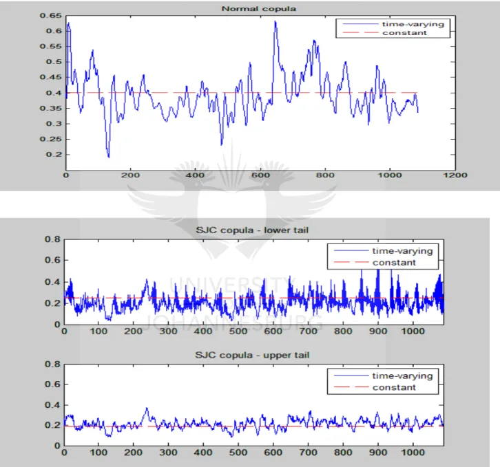
In view of this approach, instead of using simulation to assess the VaR of copulas, we employ time-varying dependence for the normal copulas to perceive the impact of VaR during the observation period under study. Time variation in the normal copula will be symbolized by 𝜌10

(𝑟ℎ𝑜₁₀). The estimates of normal copula have two forms: one constant 𝜌 and another varying over time noted by 𝜌𝑡, expressed by the following evolution function:

𝜌_𝑡 = ∇(𝑤_𝜌 + 𝛽_𝜌 𝜌_(𝑡 − 1) + 𝛼 1/10 ∑_(𝑗 = 1)^10▒𝜃^(−1) (𝑢_(𝑡 −

𝑗) ) 𝜃^(−1) (𝑣_(𝑡 − 𝑗) )) (37)

We then draw on the upper and lower tail dependence of SJC copulas to evaluate the observed VaR on the tail of distribution. The upper tail will be noted by 𝜏_𝑈 (Tau) and the lower tail noted by 𝜏𝐿 as shown in the study of Patton (2006), and are expressed as follows:

𝜏_𝑡𝑈 =∧ (𝑤_𝑈+ 𝛽_𝑈𝜏_𝑡−1𝑈 + 𝛼_𝑈. 1 10∑ |𝑢𝑡−𝑗 − 𝑣𝑡−𝑗| 10 𝑗=1 ) (38) 𝜏_𝑡𝐿 =∧ (𝑤_𝐿+ 𝛽_𝐿𝜏_𝑡−1𝐿 + 𝛼_𝐿. 1 10∑ |𝑢𝑡−𝑗− 𝑣𝑡−𝑗| 10 𝑗=1 ) (39)

It is crucial to stress that the losses are observed at the tail. The question at this point is: at which risk? This process will allow us to understand a clear level of risk among these markets so that we can aid to investors’ decision-making.

4.4 Back-testing

Applying the back-test is an essential part of the VaR model assessment process. It takes the values that have been computed by the chosen model and tests if that model can justify its application on a known portfolio.

The statistical tests are frequently two sets of groups: unconditional coverage and independence. The violations frequencies are counted by unconditional coverage when the actual return surpasses the VaR number for that date. If the VaR level is 1% from a sample of 100 VaR estimates in contradiction of actual return observations, it would be expected that one of them is a violation.

The test for independence hypothesizes that the observations are independent of each other. Based on this hypothesis, when a violation occurs for two or more successive days, we conclude that there might be a problem with the model. The following sections describe the two types of back-testing.

(29)

20 | P a g e

4.4.1 Christoffersen test

The Christoffersen test is elucidated in Christoffersen & Pelletier (2004) , and is both an independence and a likelihood-ratio test similar to the Kupiec (1995) test, in that it tests the joint assumption of unconditional coverage and independence of failures. The Christoffersen test focusing on the probability of failure rate is used in order to evaluate the estimated VaR values. The probability of failure rate in the VaR simulation is the essential point for back-testing. To conduct the test, one should first define

))

(

VaR

Pr(y

p





_t



_t



and test



p

:

H

_o



against



p

:

H

₁



.

The constraint is that



1(y

_t



VaR

(



)



has a binomial likelihood and can be given by: 𝐿(𝑃𝛼) = (1 − 𝑃𝛼₎𝑛0_(𝑃𝛼₎𝑛1 ₍₄₀₎

where 𝑛0 = ∑𝑇𝑡=𝑅1(𝑦𝑡 > 𝑉𝑎𝑅𝑡(𝛼)) and 𝑛1 = ∑𝑇𝑡=𝑅1(𝑦𝑡 < 𝑉𝑎𝑅𝑡(𝛼))

(Saltoglu, et al., 2003)

It becomes

L(



)



(1

-



)

n0



n1 under the null hypothesis. Thus, the likelihood ratio test statistic can be given in equation 41:

𝐿𝑅 = −2 ln(𝐿(𝛼))/𝐿(𝑃̂))→ 𝜒(1)𝑑 (41)

The highest benefit of this likelihood ratio test statistic is that it can reject a VaR model that generates either too many or too few clustered violations, although it needs several hundred observations in order to be accurate.

An effective estimated VaR should be below the correct value for a given percent of the cases. Likewise, there should not be any clusters of exceeding values; consequently, independence of the VaR values of each other must be observed. The last test is the combination of the first and the second test, which allows for the investigation of both of these aspects. Therefore, we may

(30)

21 | P a g e proceed with testing the VaR for the unconditional coverage and independence at the same time.

4.4.2 Kupiec test

Kupiec (1995) proposed the test of unconditional coverage, which measures whether the number of violations is compatible with the chosen confidence level. The exceptions number follows the binomial distribution, and the hypothesis test is defined as:

T x p p :    Ho

Here, p and x respectively represent the exceptions rate from the selected VaR level and the observed number of violations. T represents the number of observations. This test is shown as a LR test and could be formulated as:

𝐿𝑅_𝑈𝐶 = 2 ln (𝑃𝑥(1−𝑃̂)𝑇−𝑥

𝑃𝑥_(1−𝑃)𝑇−𝑥) (42)

The test of LR is asymptotically distributed 𝜒2 (chi-square) with one degree of freedom. Up to a confidence, level of 95%, and on the condition that the statistic exceeds the critical value (3.5), 𝐻₀ is denied and then the model seems inaccurate.

In this thesis, with 0.01confidence interval we assess and back-test the VaR model using Kupiec Christoffersen out-of-sample forecasting test, taking into account the Basel (2011) I prerequisite of a 99% confidence level.

(31)

22 | P a g e

Chapter: 5 Data, simulation and analysis

This section describes the data set used and emphasizes its major features. We also establish the steps for modelling process, as set out below:

1. First step: establishment of model and estimation of the margins of indexes of the five studies, bearing in mind their conditional mean and variance.

2. Estimate VaR via copula for four particular proposed portfolios constructed from our data.

5.1. Data description

For this thesis, our estimation of the VaR is based on the use of the copula framework of five stock indices in BRICS countries.

The data for stock indices was found in Yahoo Finance, except for JSE data, which was sourced from the national stock exchange. The sample period was from March 11th 2013 to May 16th 2017. In order to avoid downsize bias, we excluded the no-trading days in the observed markets.

The sample contained 1087 daily closing prices. Usually, we took the log-returns of each index, and multiplied by 100. The log-returns were expressed by 𝑟_𝑡 = ln ( 𝑝𝑡

𝑝𝑡−1) ∗ 100 and 𝑝𝑡

represented the value of index at a given time t. If 𝑟𝑡 was zero for at least one, this observation

was not to be considered within the series.

All stock indices have a tendency. Figure 1 below displays the evolution of the BRICS stocks market indices.

(32)

23 | P a g e Figure 5-1: The complete data set of the price indices of all stock markets

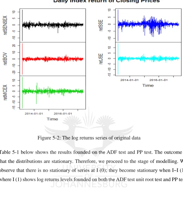
The log returns of Brazil are noted by variable retIBOV, the log returns of Russia as variable retMICEX, the log returns of India as variable retSENSEX, the log returns of China as retSSE and the log returns of South Africa as variable retJSE. However, the log differences let the series become stationary. Figure 2 presents the plot of estimated stock indices in log-differenced series.

(33)

24 | P a g e Figure 5-2: The log returns series of original data

Table 5-1 below shows the results founded on the ADF test and PP test. The outcome is that the distributions are stationary. Therefore, we proceed to the stage of modelling. We observe that there is no stationary of series at I (0); they become stationary when I~I (1), where I (1) shows log returns levels founded on both the ADF test unit root test and PP test.

(34)

25 | P a g e Table 5-1: ADF and PP unit root test results

PP Test I(1) ADF Test I(1)

SENSEX -6.999 1.2012 IBOV -9.6669 0.2492 MICEX -26.372 0.6169 SSE -5.7581 0.081 JSE -16.668 0.6693 RetSENSEX -1068.4* -24.6228* RetIBO -1230.0* -25.6189* RetMICEX -1179.9* -24.4043* RetSSE -1058.0* -23.9056* RetJSE -1134.1* -27.1819*

*stationary at 1% confidence level

The main statistical properties of the log-differenced series are shown in Table 5.2. It appears that means are close to zero and the standard deviations are very small, indicating that none of the five series has a constant term and all the data is distributed around the mean. In addition, the results indicate that no index had a significant trend over the sample period, since means are very small relative to the standard deviation of each series.

The five indices generally exhibit negative skewness (the retIBOV is, however, slightly positive) and substantial excess kurtosis. The negative skewness indicates that the negative returns happen more often than large positive returns. The means and volatilities are very similar, as expected.

(35)

26 | P a g e Table 5-2: Descriptive statistics of daily returns stock indices *

Stock Market Index retSENSEX retIBOV retMICEX retSSE retJSE

Mean 0.04075016 0.01470724 0.02580113 0.02744670 0.02549411 Std Dev 1.048581 1.760939 1.325140 1.631826 1.116976 Kurtosis 31.70484 54.58105 30.57703 9.17702 47.63502 Skewness -0.52911225 0.09862383 -0.98869907 -1.2064227 -0.46087331 Min -12.31295 -23.14691 -15.34293 -11.85597 -14.56619 Max 11.61895 23.32962 13.04419 10.15689 13.85882 Jarque-Bera Statistic 45719.8042** * 135330.6744* ** 42655.6506*** 4093.691*** 103118.0737* ** Linear correlation 0.559735117 -0.0792158 0.027071103 -0.0091878 --- Number of obs 1086 1086 1086 1086 1086

Notes: The Jarque-Bera statistics: *** indicate that the null hypothesis (of normal distribution) is rejected at a 1% significance level. Source: Author’s calculations

ret represents log-differencing. Kurtosis and skewness is three and zero for normal distribution (Gaussian). The Jarque-Bera(JB) test invented by Jarque and Bera (1980), is a statistical test for normality.

𝐽𝐵 =𝑇

6(𝑆𝐾

2₊(𝐾𝑉−3)2

4 ),

Where SK denotes the sample skewness, KU the sample kurtosis, and T the sample size. The null hypothesis states that the sample is drawn from a normal distribution. The appropriate test statistic is calculated as 𝐽𝐵~ 𝜒₂2

(36)

27 | P a g e Often the correlation is still used in finance. Pearson’s correlation coefficient 𝜌𝑥𝑦𝜖[−1,1].

Person’s 𝜌𝑥𝑦 mesures linear dependence between X and Y. Pearson’s correction can be

interpreted as the slope of the regression line of X and Y.

The Jarque-Bera test calculates whether the residuals have a normal distribution, and linear correlation is estimated with 𝜌_𝑋𝑌 = 𝐶𝑂𝑉(𝑋, 𝑌) 𝜎⁄ _𝑋𝜎_𝑌.

The Q-Q-plots in Figure 5-3 show that the stock indices might not be normal. The null hypothesis of Jarque-Bera test has been rejected under 0.01 significant level, which means that neither of the series are unconditionally normally distributed.

(37)

28 | P a g e Figure 5-3: QQ-plots of the returns of the stock market indices versus normal density Linear correlation between the five indices is provided in Table 5-3. The retJSE-retSENSEX have the highest correlation (0.56) followed by the retIBOV-retMICEX (0.46). Between the retSSE indices and retIBOV, retSSE and retMICEX indices, the correlation is still fair (between 0.23 and 0.25). These results suggest that there is some connection between the indices of BRICS markets. These values illustrate a strong uphill linear relationship and thus indicate that copulas can be applied to improve forecasting with marginal distribution affects.

(38)

29 | P a g e Table 5-3: Linear correlation between the five returns of BRICS indices

retSENSEX RetIBOV RetMICEX RetSSE retJSE

RetSENSEX 1 -0.1104394 -0.006982222 0.01947642 0.55973512

RetIBOV -0.1104394 1 0.463888581 0.25101459 -0.07921580

RetMICEX -0.006982222 0.463888581 1 0.22584953 0.02707110

RetSSE 0.019476417 0.2510146 0.225849529 1 -0.00918078

RetJSE 0.559735117 -0.0792158 0.027071103 -0.0091878 1

These correlations between different stock indexes, as presented in Figures 5-4, 5-5, 5-6 and 5-7 below, are not constant and differ in tails, except for SSE. Thus, complex method like copulas are required to estimate portfolio VaR with marginal distribution effects.

Figure 5-4: Plot of JSE and SENSEX

(39)

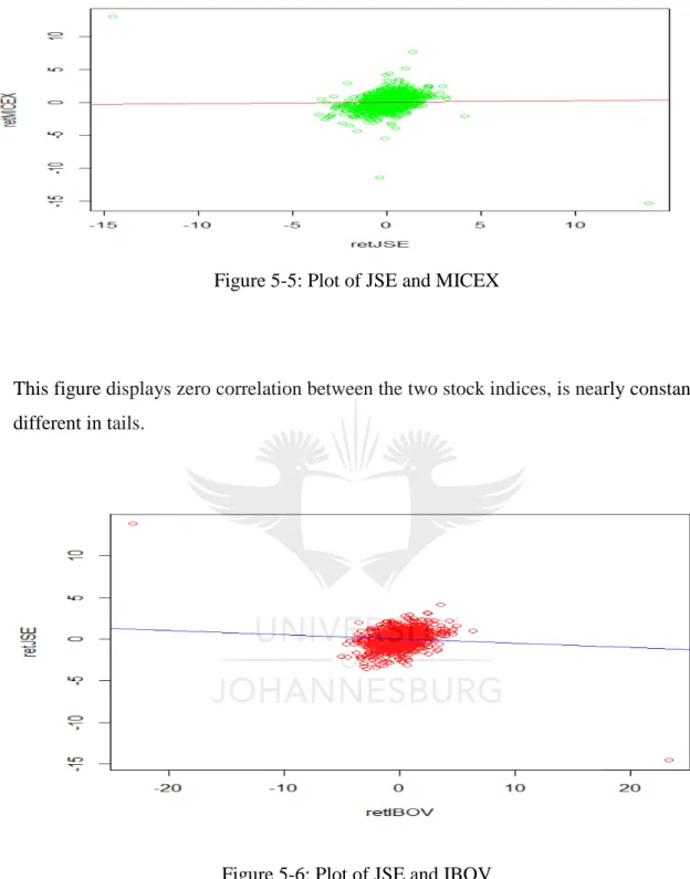
30 | P a g e Figure 5-5: Plot of JSE and MICEX

This figure displays zero correlation between the two stock indices, is nearly constant and different in tails.

Figure 5-6: Plot of JSE and IBOV

The correlation is negative between the two stock indices; this correlation is not constant but it is different in tails.

(40)

31 | P a g e Figure 5-7: Plot of JSE and SSE

There is negative correlation between these two indices, and this correlation is nearly constant The estimates of multivariate patterns are performed in pairs. More precisely, the estimation of the joint distribution via copulas is carried out between the FTE/JSE and each of the other indices. Results show that South Africa shows its higher interdependency with India (SENSEX) than Russia (MICEX), and is negatively correlated with Brazil (IBOV) and China (SSE). These results will, however, be discussed later. The main goal at this point is to measure and evaluate the dependence structure between the FTE/JSE and the other indices.

(41)

32 | P a g e

5.2 The models for the marginal distribution

Before the estimation of copulas, we fitted the data through marginal garch distribution and the residuals of the marginal were used to estimate copulas.

It is necessary to fit an appropriate marginal distribution to the residuals before we estimate the copula model. We fitted the AR (1,0)-GARCH (1,1) models for each series as initials models with normal and t-distributions. First, we fitted retSENSEX, retIBOV, retMICEX, retSSE and retJSE index returns into models (4), (5) and (6) or (7), and then used the results to obtain the probability integral transform, U and V.

A basic AR (1,0)-GARCH (1,1) model for marginal variables was used for each index, as it is the common model used to describe financial time series (Diebold et al., 1998). The results of the parameters of these marginal distributions are provided in Table 5-4. All values except for the AR (1) values seem to significantly differ from zero.

In Table 5-4, The AR (1) terms for the retIBOV, retMICEX, retSSE and retJSE are not significantly different from zero. However, as stated before, the AR (1) terms are kept in the model so the first part is not only the constant parameter. All constant parameters are positively not significant from zero, so all indices increase over time. In all five cases, the sum of the lagged e2 and lagged variance is smaller than 1, suggesting that the GARCH model is stationary.

(42)

33 | P a g e Table 5-4: Results for AR (1)-GARCH (1,1) – Normal estimations1

retSENSEX retIBOV retMICEX RetSSE RetJSE

AR (1)-GARCH (1,1)-N Constant µ1 0.079229 (0.029986)* 0.032961 (0.045392) 0.026057 (0.035227) 0.033253 (0.030518) 0.050936 (0.027127) AR(1) ϕ1 0.088153 (0.035551)* -0.014852 (0.034978) -0.059441 (0.031074) 0.010335 (0.033391) -0.000297 (0.034626) GARCH constant α1 0.046230 (0.016890)* 0.104622 (0.037077)* 0.0000 (0.000168) 0.006570 (0.003551) 0.018827 (0.006542)* Lagged e2 β1 0.081594 (0.019882)* 0.043470 (0.009564)* 0.002076 (0.000144)* 0.057346 (0.009119)* 0.047993 (0.008626)* Lagged variance ɤ1 0.869711 (0.028427)* 0.907210 (0.020616)* 0.996924 (0.0001760* 0.939037 (0.008563)* 0.927799 (0.012119)* Degrees of freedom ɣ1 --- --- --- --- --- Log likelihood -1501.006 -2053.164 -1810.769 -1800.346 -1539.914 AIC 2.7735 3.7904 3.3440 3.3248 2.8451 * Significance level = 0.05

(43)

34 | P a g e Table 5-5: Represents the estimation of AR (1)-GARCH (1,1) – student t2

AR-GARCH-t retSENSEX RetIBOV retMICEX retSSE retJSE

Constant µ1 0.061715 (0.026422)* 0.021901 (0.041002) 0.035106 (0.032073) 0.069156 (0.026426)* 0.057612 (0.024085)* AR(1) ϕ1 0.089702 (0.028848)* -0.017330 (0.031428) 0.042350 (0.031517) 0.014724 (0.027245) -0.003945 (0.031157) GARCH constant α1 0.062619 (0.028218)* 0.277313 (0.155184) 0.337042 (0.144985)* 0.023540 (0.010183)* 0.047223 (0.017546)* Lagged e2 β1 0.058358 (0.021108)* 0.083078 (0.029691)* 0.129385 (0.048138)* 0.082126 (0.020950)* 0.106164 (0.026211)* Lagged variance ɤ1 0.872201 (0.042811)* 0.794917 (0.085624)* 0.630458 (0.128276)* 0.916874 (0.017155)* 0.847416 (0.032964)* Degrees of freedom 𝑣1 4.570925 (0.659187)* 6.854718 (1.265258)* 5.035559 (0.694494)* 3.357759 (0.392215)* 5.671626 (0.911972)* Log likelihood -1409.835 -1953.851 -1647.762 -1712.07 -1435.9 AIC 2.6074 3.6093 3.0456 3.1640 2.6554

(44)

35 | P a g e In Table 5-5, all parameters except parameters AR (1)-retSENSEX are not significant at the level 0.05 for retIBOV, retMICEX, retSSE and retJSE indices returns. For all five cases, the lagged sum e2 and lagged variance are not greater than one, suggesting that the GARCH model is stationary.

The parameters estimated of the GARCH-t and GARCH-N models are done for all indices, as shown above. Considering the maximum log-likelihood, we believe that the student t-distribution fits for all BRICS indices.

) ( ₁_, ₁

1 

 _t _t _T

t F X F

u and v_t F₂_,_t(X₂_,_,_t F_T_₁) where

F

₁_,_t and

F

₂_,_tare marginal distributions conditioned to Ft-1, and the information variable up to time t-1. If the models were properly

definite, then both series would be standard uniform. The fit thus seems good.

The Ljung-Box test used on the residuals of the GARCH-t and GARCH-N models does not reject the null hypothesis (𝐻₀) of null autocorrelations from lag one to 10 for the residuals for both series at a significance level of 5%. The Ljung-Box test also does not reject the 𝐻0 from

lag one to 10 for the square of the residuals series at the 5% significance level. Therefore, we consider the models to be adequate. Table 5-6 shows the p-value of standardized squared residuals and standardized residuals for all returns.

(45)

36 | P a g e Table 5-6: P-value for standardized squared residuals and standardized residuals

Standardized Residuals Standardized Squared Residuals

GARCH-Normal GARCH-Student-t GARCH-Normal GARCH-Student-t

retSENSEX 0.173 0.089 0.237 0.010

retIBOV 0.789 0.953 0.173 0.960

retMICEX 0.893 0.869 0 0.999

RetSSE 0.486 0.625 0.688 0.908

RetJSE 0.009 0.069 0.049 0.958

We observe no autocorrelation in the residuals, nor in the squ