Statistical Methods in Neuroimaging Genetics: Pathways Sparse Regression and Cluster Size Inference

(1)

Statistical Methods in Neuroimaging Genetics:

Pathways Sparse Regression

and Cluster Size Inference

A thesis presented for the degree of

Doctor of Philosophy of the University of London and the Diploma of Imperial College

by

Matthew Silver

Department of Mathematics Imperial College

180 Queen’s Gate, London SW7 2BZ

(2)

(3)

ii

I certify that this thesis and the research to which it refers are the product of my own work, and that any ideas or quotations from the work of other people, published or otherwise, are fully acknowledged in accordance with the standard referencing practices of the discipline.

(4)

Copyright

Copyright in the text of this thesis rests with the Author. Copies (by any process) either in full, or of extracts, may be made only in accordance with instructions given by the Author and lodged in the doctorate thesis archive of the college central library. Details may be obtained from the Librarian. This page must form part of any such copies made. Further copies (by any process) of copies made in accordance with such instructions may not be made without the permission (in writing) of the Author. The ownership of any intellectual property rights which may be described in this thesis is vested in Imperial College, subject to any prior agreement to the contrary, and may not be made available for use by third parties without the written permission of the University, which will prescribe the terms and conditions of any such agreement. Further information on the conditions under which disclosures and exploitation may take place is available from the Imperial College registry.

(5)

iv

Acknowledgements

I am indebted to my Ph.D supervisor, Dr Giovanni Montana, for his advice and guidance. Thanks to him, I have made the journey from a position of scant understanding, to one of at least moderate understanding of the world of statistics applied to the analysis of large biological datasets. I am also grateful to the Wellcome Trust, who generously funded my studies and research.

In addition I would like to acknowledge contributions from external collaborators in three of the studies described in this thesis:

1. For the Alzheimer’s pathways study described in Section 3.5, image pre-processing and analysis was carried out by Eva Janousova, at the time visiting Imperial Col-lege from the Institute of Biostatistics and Analyses, Masaryk University, Brno in the Czech Republic, and by Dr Xue Hua and Professor Paul Thompson from the Laboratory of Neuro Imaging, Department of Neurology at the UCLA School of Medicine, USA. ADNI Genotype data was extracted from imputed genotypes used in two previous studies (Vounou et al., 2011; Stein et al., 2010a).

2. For the HDL-C study described in Section 4.3, non-imputed genotype data was pro-vided by Professor YY Teo and Cheng Peng from the Department of Statistics and Applied Probability, University of Singapore.

3. For the study investigating control of false positive rates using cluster size inference in Chapter 6, which began as a final project for an MSc in Bioinformatics and Theo-retical Systems Biology at Imperial College, extensive help and support was provided by Dr Thomas Nichols at the Department of Statistics & Warwick Manufacturing Group, University of Warwick, UK.

Finally, I would like to thank my immediate family, Bryher, Morwenna, Rosie and Elo¨ıse, for their boundless patience and support throughout.

(6)

ADNI Data Use

Neuroimaging and genotype data used in a number of studies in this thesis were obtained from the Alzheimers Disease Neuroimaging Initiative (ADNI) database (adni.loni.ucla.edu). As such, the investigators within the ADNI contributed to the design and implementation of ADNI and/or provided data but did not participate in analysis or writing of any part of this thesis. A complete listing of ADNI investigators can be found at http://adni.loni.ucla.edu/wp-content/uploads/how to apply/ADNI Acknowledgement List.pdf.

ADNI is funded by a National Institutes of Health Grant U01 AG024904, and by the Na-tional Institute on Aging, the NaNa-tional Institute of Biomedical Imaging and Bioengineering, and through generous contributions from the following: Abbott; Alzheimers Association; Alzheimers Drug Discovery Foundation; Amorfix Life Sciences Ltd.; AstraZeneca; Bayer HealthCare; Bio-Clinica, Inc.; Biogen Idec Inc.; Bristol-Myers Squibb Company; Eisai Inc.; Elan Pharmaceuticals Inc.; Eli Lilly and Company; F. Hoffmann-La Roche Ltd and its affiliated company Genentech, Inc.; GE Healthcare; Innogenetics, N.V.; Janssen Alzheimer Immunotherapy Research & Develop-ment, LLC.; Johnson & Johnson Pharmaceutical Research & Development LLC.; Medpace, Inc.; Merck & Co., Inc.; Meso Scale Diagnostics, LLC.; Novartis Pharmaceuticals Corporation; Pfizer Inc.; Servier; Synarc Inc.; and Takeda Pharmaceutical Company. The Canadian Institutes of Health Research is providing funds to support ADNI clinical sites in Canada. Private sector contributions are facilitated by the Foundation for the National Institutes of Health (www.fnih.org). The grantee organization is the Northern California Institute for Research and Education, and the study is coor-dinated by the Alzheimer’s Disease Cooperative Study at the University of California, San Diego. ADNI data are disseminated by the Laboratory for Neuro Imaging at the University of California, Los Angeles. This research was also supported by NIH grants P30 AG010129 and K01 AG030514.

(7)

vi

Abstract

In the field of neuroimaging genetics, brain images are used as phenotypes in the search for genetic variants associated with brain structure or function. This search presents a formidable statistical challenge, not least because of the very high dimensionality of geno-type and phenogeno-type data produced by modern SNP (single nucleotide polymorphism) ar-rays and high resolution MRI. This thesis focuses on the use of multivariate sparse regres-sion models such as the group lasso and sparse group lasso for the identification of gene pathways associated with both univariate and multivariate quantitative traits.

The methods described here take particular account of various factors specific to path-ways genome-wide association studies including widespread correlation (linkage disequi-librium) between genetic predictors, and the fact that many variants overlap multiple path-ways. A resampling strategy that exploits finite sample variability is employed to provide robust rankings for pathways, SNPs and genes. Comprehensive simulation studies are pre-sented comparing one proposed method,pathways group lasso with adaptive weights, to a popular alternative. This method is extended to the case of a multivariate phenotype, and the resultingpathways sparse reduced-rank regressionmodel and algorithm is applied to a study identifying gene pathways associated with structural change in the brain characteris-tic of Alzheimer’s disease. The original model is also adapted for the task of ’pathways-driven’ SNP and gene selection, and this latter model, pathways sparse group lasso with

adaptive weights, is applied in a search for SNPs and genes associated with elevated lipid

levels in two separate cohorts of Asian adults.

Finally, in a separate section an existing method for the identification of spatially ex-tended clusters of image voxels with heightened activation is evaluated in an imaging ge-netic context. This method, known as cluster size inference, rests on a number of

(8)

assump-trolled outside of a narrow range of parameters related to image smoothness and activation thresholds for cluster formation.

(9)

viii

List of Figures

1.1 Schematic representation of points of common genetic variation between

individuals . . . 7

1.2 Pairwise correlation (LD) patterns between 420 SNPs on a 500kb stretch of human chromosome 5 . . . 8

1.3 Schematic of genes acting together in a functional pathway . . . 12

1.4 Schematic illustration of the SNP to pathway mapping process . . . 14

1.5 Imaging genetic analysis . . . 18

1.6 MULM in imaging genetic analysis . . . 22

2.1 Lasso coefficient estimation with two predictors . . . 30

2.2 Group lasso - schematic illustration of distribution of causal SNPs . . . 37

2.3 The problem of overlapping pathways . . . 40

2.4 SNP to pathway mapping. . . 58

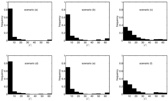
2.5 Frequency distribution of ADNI SNPs by number of pathways they map to 59 2.6 Distributions of_|C|across500MC simulations for each of the6scenarios tested . . . 61

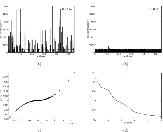
2.7 Application of bias-adjusted weighting procedure to the data used in the simulation study . . . 63

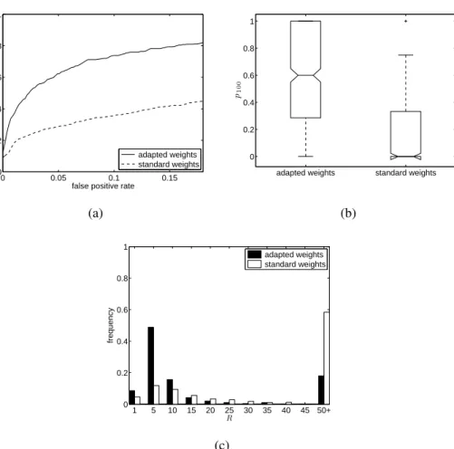
2.8 Ranking performance using adapted weights . . . 65

2.9 ROC curves . . . 68

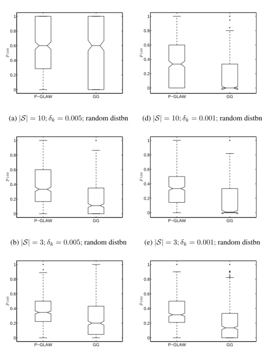
2.10 Box plots of distribution of ranking power,p100, across500simulations . . 69

2.11 Distribution of the power-adjusted, normalised, weighted ranking score,R, across500simulations . . . 70

3.1 Reduced-rank regression model. . . 78

3.2 Reduced-rank regression latent factors. . . 79

3.3 PsRRR Simulation study 1 . . . 89

3.4 PsRRR simulation study 2 . . . 91

3.5 Mapping SNPs to pathways . . . 97

3.6 ADNI/KEGG pathway sizes and SNP overlaps . . . 98

(13)

LIST OF FIGURES 2

3.8 Sample mean(left)and standard deviation(right)of slope coefficients for

the 2 subject groups . . . 101

3.9 Imaging signature characteristic of AD . . . 102

3.10 3D multi-dimensional scaling plot illustrating the spread of imaging signa-tures across ADs and CNs . . . 103

3.11 Measure of extent to which genes previously linked to AD are enriched in highly-ranked pathways . . . 107

4.1 Sparsity patterns enforced by the group lasso and sparse group lasso . . . . 113

4.2 SGL vs Lasso. Comparison of power to detect 5 causal SNPs . . . 122

4.3 SGL vs Lasso. Distribution over 500 MC simulations of power to detect 5 causal SNPs . . . 123

4.4 Two pathways with partially overlapping causal SNPs . . . 125

4.5 SGL Simulation Study with overlapping pathways . . . 129

4.6 SGL-CGD vs SGL-BCGD performance, measured across 2000 MC simu-lations . . . 131

4.7 SP2 dataset. SNP to pathway mapping. . . 138

4.8 SiMES dataset. SNP to pathway mapping. . . 138

4.9 Empirical and null pathway selection frequency distributions for all 185 KEGG pathways with the SP2 dataset . . . 141

4.10 Empirical and null SNP selection frequency distributions with the SP2 dataset142 4.11 SP2 dataset: Scatter plots comparing empirical and null selection frequencies144 4.12 SiMES dataset: Scatter plots comparing empirical and null selection fre-quencies . . . 148

4.13 Selection frequency distributions for the SiMES dataset . . . 149

4.14 Comparison of top-kSP2 and SiMES pathway rankings . . . 154

4.15 Comparison of top-kSP2 and SiMES gene rankings . . . 157

6.1 Non-stationary image simulation . . . 179

6.2 Accuracy of estimation ofc, the theoretical number of clusters under RFT . 189 6.3 Distribution of voxel-wise FWHM for ADNI images smoothed with 6mm (left) and 12mm (right) Gaussian smoothing kernels . . . 191

(14)

List of Tables

1.1 SNP association test in a case-control study . . . 9

2.1 Scenarios tested in simulation study . . . 60

2.2 GL estimation times in seconds . . . 62

2.3 Selected ranking performance measures for P-GLAW and GG . . . 66

2.4 Proportion of500simulations withR <10andR <3 . . . 71

3.1 Empirical phenotypicSN Rvalues . . . 88

3.2 Empirical phenotypicSN Rvalues for Simulation study 2 . . . 90

3.3 Available scans at 6, 12 and 24 months for the ADNI-1 dataset (down-loaded on February 28, 2011) . . . 95

3.4 AD genes included in this study . . . 99

3.5 Top 30 pathways, ranked by pathway selection frequency. . . 104

3.6 Top 30 SNPs and genes, respectively ranked by SNP and gene selection frequency, using lasso sRRR . . . 106

4.1 Simulation Study 2: Mean number of pathways and SNPs selected by each model at each effect size,γ, across 2000 MC simulations. . . 130

4.2 Genotype and phenotype information corresponding to the SP2 and SiMES datasets used in the study. . . 136

4.3 SNP and gene to pathway mappings for the SP2 and SiMES datasets. . . . 139

4.4 Separate combinations of the P-SGLAW regularisation parameters, λand αused for analysis of the SP2 dataset . . . 140

4.5 SP2 dataset: Pearson correlation coefficients(r)and p-values . . . 143

4.6 SP2 dataset: Top 30 pathways, ranked by pathway selection frequency . . . 146

4.7 SP2 dataset: Top 30 SNPs and genes ranked by SNP and gene selection frequency . . . 147

4.8 SiMES dataset: Pearson correlation coefficients(r)and p-values . . . 148

4.9 SiMES dataset: Top 30 pathways, ranked by pathway selection frequency . 150 4.10 SiMES dataset: Top 30 SNPs and genes ranked by SNP and gene selection frequency . . . 151

4.11 Consensus set of pathways for SP2 and SiMES datasets withk = 25 . . . . 155

(15)

LIST OF TABLES 4

4.13 Consensus set of genes for SP2 and SiMES datasets withk= 244 . . . 158

4.14 Summary of SNPs analysed and ranked in SP2 and SiMES datasets. . . 159

4.15 Top 30 SNPs ranked in both SP2 and SiMES datasets, ranked in order of mean ranking,ψSN P (4.28). . . 160

6.1 FWER-corrected results - real (ADNI) images . . . 184

6.2 FDR-corrected results - real (ADNI) images . . . 185

6.3 Results - simulated images . . . 187

(16)

List of Publications

Much of the material to be found in this thesis is covered in the following published papers:

1. Silver M, Janousova E, Hua X, Thompson, P and Montana G (2012). Identifica-tion of gene pathways implicated in Alzheimers disease using longitudinal imaging phenotypes with sparse regression.NeuroImage63.3, pp. 16811694.

2. Silver M and Montana G (2011). Fast identification of biological pathways associ-ated with a quantitative trait using group lasso with overlaps.Statistical Applications

in Genetics and Molecular Biology11.1.

3. Silver M and Montana G (2011). Pathway selection for GWAS using the group lasso with overlaps. In International Conference on Bioscience, Biochemistry and

Bioinformatics. Vol. 5, pp. 114117.

4. Silver M, Montana G and Nichols, T E (Sept. 2010). False positives in neuroimaging genetics using voxel-based morphometry data.NeuroImage54.2, pp. 9921000.

(17)

6

Chapter 1

Introduction

1.1

Gene association mapping

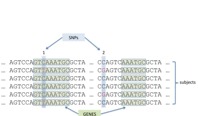
Since the publishing of the first draft of the human genome, a huge amount of effort has been expended in the hunt for genetic variation associated with human disease. Much of this work has focused on the identification of single points of variation, known as single nucleotide polymorphisms or SNPs, where common variation is observed in the human population (see Figure 1.1). Parallel advances in sequencing technology and the detailed cataloguing of SNPs for diverse human populations have led to the identification of 100s of SNPs affecting an array of common diseases and traits (Green et al., 2011; Altshuler, Daly, and Lander, 2008).

In modern genome-wide association studies (GWAS), 100s or 1000s of individuals are genotyped at up to a million or more SNPs across the genome. This ‘hypothesis-free’ ap-proach to searching for genetic variants in GWAS has been greatly aided by the ability to exploit patterns of widespread correlation or linkage disequilibrium (LD) between genetic markers belonging to unrelated individuals. Different human sub-populations can be char-acterised by these distinctive LD patterns, which have a block-like structure, arising from the relatively few sexual recombination events that have occurred throughout recent hu-man history (see Figure 1.2). For a given huhu-man sub-population, the presence of these LD blocks orhaplotypesenables single ‘tagging’ SNPs to be used as proxies for other, ungeno-typed variants, dramatically decreasing the number of variants that need to be genoungeno-typed

(18)

… AGTCCAGTCAAATGCGCTA … CCAGTCAAATGCGCTA …

… AGTCCAGT

T

AAATGCGCTA … C

G

AGTCAAATGCGCTA …

… AGTCCAGTCAAATGCGCTA … CCAGTCAAATGCGCTA …

… AGTCCAGTCAAATGCGCTA … C

G

AGTCAAATGCGCTA …

… AGTCCAGT

T

AAATGCGCTA … CCAGTCAAATGCGCTA …

GENES SNPs

subjects

1 2

Figure 1.1: Schematic representation of points of common genetic variation between individuals. Letters ACGT represent single nucleotides that make up the human genome. Extended stretches of nucleotides can be grouped intogenes, broadly classified as functional units within the genome. Single nucleotide polymorphisms or SNPs, are genetic loci at which there is common variation between individuals in the human population, typically defined as variants whose minor ‘allele’ (here marked in red) occurs with a frequency> 1%. An individual has two copies of each allele, and so may possess0,1or2minor alleles. SNPs may occur within genes (SNP 1) or between genes (SNP 2).

(19)

1.1 Gene association mapping 8

(The International HapMap Consortium, 2005). Variants identified using this approach will however typically have only an indirect relationship to the true causal variant(s) that they tag (Hirschhorn and Daly, 2005). For this reason, this approach may also come at the cost of reduced power, compared to fine-mapping studies that include all SNPs in a genomic region of interest. The presence of LD can also lead to inflated numbers of false positives, due to spurious associations arising from SNPs in LD with causal SNPs.

Figure 1.2: Pairwise correlation (LD) patterns between 420 SNPs on a 500kb stretch of human chromosome 5. High pairwise correlation in the sample population is marked in brown. Blocks of strong correlation, known ashaplotypes, are marked by the black outline. Plot taken from Altshuler, Daly, and Lander (2008).

Genetic variation between subjects is generally measured by recording the number of minor alleles possessed by each individual, a SNP’s minor allele being defined as the less common variant in the sample (variants marked in red in Figure 1.1). Since individuals inherit two copies of each allele, one from the mother and one from the father, each subject may possess zero, one or two minor alleles. Thus in a study with N subjects genotyped at P SNPs, we can denote the minor allele count for SNP j observed on individual i as xij ∈ {0,1,2}, i= 1, . . . , N;j = 1, . . . , P.

The standard statistical approach is then one of mass univariate testing, where the hy-pothesis that minor alleles are associated with a particular trait orphenotypeis tested, one SNP at a time. In a case-control study for example, we might test the hypothesis that minor alleles are more likely to be found in cases than controls by testing for independence of rows and columns in a2_×2contingency table, using a χ2

(20)

xj 0 1,2 total cases d0 d12 D controls c0 c12 C total n0 n12 N (a) Observed xj 0 1,2 total cases n0D/N n12D/N D controls n0C/N n12C/N C N (b) Expected

Table 1.1: Association test for SNPjin a case-control study. (a)d0, d12represent observed number

of cases withxj = 0, or xj ∈ {1,2}, respectively. c0, c12 represent the same for controls. (b)

Expected values under the null, i.e. where rows and columns in (a) are independent. The hypothesis that minor alleles are associated with disease status is tested by observing that P

(Observed₋ Expected)2_/Expected_∼_χ2

1 under the null.

genetic models, assuming for example recessive or dominant genetic effects can be tested by changing the column categories. An alternative strategy for testing associations in case-control studies is to code phenotypes asyi ∈ {0,1}for cases and controls respectively, and

use a logistic regression model, logit(πi) =β0+β1xij, where logit(πi) =log(πi/(1−πi)

andπiis the disease risk of theith individual. Here we assume an additive genetic model,

whereby disease risk increases in proportion with the number of minor alleles. We can test the null hypothesis that there is no association between disease status,H0 : ˆβ1 = 0, using a

likelihood-ratio test. The use of a logistic regression model has the advantage of allowing easy incorporation of model covariates, such as age or sex.

The search for SNPs, known as ‘quantitative trait loci’ (QTL), influencingquantitative

traits, i.e. those that vary continuously, for example blood pressure or blood lipid levels,

is also gaining momentum as a potentially more powerful way to study the underlying causes of complex disease (Plomin, Haworth, and Davis, 2009). For quantitative traits, the association of SNP minor alleles with a phenotype is established using a quantitative trait test of association (QTT). For example by assuming a linear modelyi = β0+xijβj +i,

we can perform a t-test on the SNP regression coefficient βj to test the null hypothesis

H0 :βj = 0. Once again this model can easily be extended to include covariates.

A major limitation of the mass univariate testing approach in GWAS arises from the very large number of SNPs, and hence hypotheses that must be tested. In order for the number of false positives to be adequately controlled, some correction to the single-SNP threshold for significance,α, corresponding to the probability that a single test will yield a false positive association, must be applied. If we performP such tests across the genome,

(21)

1.1 Gene association mapping 10

and further assume that each test is independent, the corresponding chance, genome-wide, for such a false positive finding is thenαGW _{= 1}₋₍₁₋_α)P_{. This leads to the familiar}

Bonferroni correction, αGW ₌ _α/P_{, which at the} _α _{= 0.05} _{level yields a significance}

threshold,αGW = 10−7 for a typical GWAS withP = 500,000 . Such a stringent thresh-old for the achieving of genome-wide significance substantially reduces the power to detect associations (Altshuler, Daly, and Lander, 2008). The presence of widespread correlation between markers due to LD means that tests are in fact not independent, so that the Bon-ferroni correction is likely to be too conservative. One solution is to approximate the false positive rate by comparing empirical p-values with a null distribution generated from the same dataset, but with multiple phenotype permutations. Here LD patterns are preserved while the phenotype-genotype association is broken (Balding, 2006). Another approach is to increase power by accepting a higher risk of false positives by controlling the expected number of false discoveries as aproportionof positive tests, using the false discovery rate (FDR) (Benjamini and Hochberg, 1995).

In contrast to univariate, ‘one SNP at a time’ methods, multivariate or multilocus meth-ods allow all SNPs to be considered in the model at the same time, which can aid the identification of weak signals while diminishing the importance of false ones. Multilo-cus or haplotype methods test the association of haplotypes, rather than individual SNPs, with phenotypes, and are thus able to implicitly exploit dependencies between SNPs, while reducing the number of tests to be performed (Duggal et al., 2008; Balding, Waldron, and Whittaker, 2006). Another approach is to extend the previous, single SNP regression model described earlier, to a multiple regression model, in which all SNPs are modelled together. Thus for a quantitative trait we have the multiple linear regression (MLR) model, yi = β0+PP_j₌₁xijβj +i. The use of multiple regression models in GWAS, while

the-oretically attractive, is however problematic in practice. Firstly, in GWAS, the number of SNPs is typically much greater than the sample size, so that estimates for the SNP regres-sion coefficients βj, j = 1, . . . , P, are not uniquely defined. Secondly, even where SNP

coefficients are estimable, LD or multicollinearity between SNPs renders such estimates unreliable (Hastie, Tibshirani, and Friedman, 2008).

One solution is to use some form of regularisation or constraint on the coefficient vector β = (β1, . . . , βP). Types of regularisation include ridge regression (Hoerl and Kennard,

(22)

1970), lasso regression (Tibshirani, 1996) and the elastic net (Zou and Hastie, 2005), each of which provides coefficient estimates with different characteristic properties (see Sec-tion 2.1). The lasso is a particularly attractive opSec-tion for GWAS, since the lasso constraint imposes sparse estimates forβ, in that many individual coefficient estimates are precisely zero. For this reason, the lasso, and related approaches such as stepwise regression (Hester-berg et al., 2008) are often described as performing ‘model selection’, since they highlight a subset of important predictors. Since its first application in GWAS (Wu et al., 2009), the lasso and related sparse regression models have been used to tackle a variety of problems in biomarker discovery. Of particular note in the present context is their use in imag-ing genetics for the identification of SNPs associated with high-dimensional neuroimagimag-ing phenotypes (Bunea et al., 2011; Kohannim et al., 2012a; Vounou, Nichols, and Montana, 2010).

1.2

The gene pathways approach

Gene variants identified in GWAS have so far uncovered only a relatively small part of the known heritability of most common diseases (Visscher et al., 2012). This has focused attention on the need to develop new methodological approaches. A number of factors that might explain this ‘missing heritability’ have been suggested, including the failure of many current models to capture the presence of gene-gene and gene-environment interactions, of multiple SNPs with small effect and of rare variants (Visscher et al., 2012; Manolio et al., 2009; Goldstein, 2009).

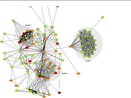
One promising approach uses prior information on functional structure present within the genome. This is motivated by the observation that in many cases disease states are likely to be driven by multiple genetic variants of small to moderate effect, mediated through their interaction in molecular networks or pathways (Figure 1.3), rather than by the effects of a few, highly penetrant mutations (Schadt, 2009). Where this assumption holds, the hope is that by considering the joint effects of multiple variants acting in concert, pathways gene association studies (PGAS) will reveal aspects of a disease’s genetic architecture that would otherwise be missed when considering variants individually (Wang, Li, and Hakonarson, 2010; Fridley and Biernacka, 2011). Other potential benefits of PGAS include:

(23)

1.2 The gene pathways approach 12

Figure 1.3: Schematic of genes acting together in a functional pathway. Coloured nodes represent genes, and edges represent possible interactions between genes. Note that pathways can interact, and genes may belong to multiple pathways.

• the ability to accommodate genetic heterogeneity, where causal markers accumulate within genes or pathways, but vary between individuals, so that marginal effects are reduced across the sample as a whole (Holmans et al., 2009)

• the ability to compare results across studies genotyping different variants, that may nonetheless be mapped to common pathways (Cantor, Lange, and Sinsheimer, 2010; Ma and Kosorok, 2010)

• better elucidation of disease mechanisms by providing a biological interpretation of association results (Cantor, Lange, and Sinsheimer, 2010)

• identification of targets for drug or other therapeutic interventions through the iden-tification of disease implicated pathways (Hirschhorn, 2009).

First developed in the context of gene expression studies (Mootha et al., 2003), pathways-based methods have more recently been extended to the analysis of GWAS data (Holmans et al., 2009; Luo et al., 2010; Lango Allen et al., 2010; Lambert et al., 2010). This has led

(24)

to the identification of putative causal pathways for a number of diseases including Parkin-son’s Disease (Lesnick et al., 2007), Crohn’s Disease (Wang et al., 2009b) and rheumatoid arthritis (Eleftherohorinou et al., 2011).

PGAS methods rely on prior information mapping SNPs to functional networks or path-ways. Since pathways are typically defined as groups of interacting genes, SNP to pathway mapping is a two-part process, requiring both the mapping of genes to pathways, and of SNPs to genes. A consistent strategy for this mapping process has however yet to be es-tablished, a situation compounded by a lack of agreement on what constitutes a pathway in the first place (Cantor, Lange, and Sinsheimer, 2010).

The number and size of databases devoted to classifying genes into pathways is grow-ing rapidly, as is the range and diversity of gene interactions considered (see for exam-ple http://www.pathguide.org/). Databases such as those provided by KEGG (http://www. genome.jp/kegg/pathway.html), Reactome (http://www.reactome.org/) and Biocarta (http: //www.biocarta.com/) classify pathways across a number of functional domains, for ex-ample apoptosis, cell adhesion or lipid metabolism; or crystallise current knowledge on specific disease-related molecular reaction networks. Strategies for pathways database as-sembly range from a fully-automated text-mining approach, to that of careful curation by experts. Inevitably therefore, there is considerable variation between databases, in terms of both gene coverage and consistency (Soh et al., 2010), so that the choice of database(s) will itself influence results in PGAS.

The mapping of SNPs to genes adds a further layer of complexity, since although many SNPs may occur within gene boundaries, in a typical GWAS, the vast majority of SNPs will reside in inter-genic regions (see Figure 1.1). In an attempt to include variants potentially residing in functionally significant regions lying outside gene boundaries, SNPs may be mapped to nearby genes using various distance thresholds. Various values for SNP to gene mapping distances, measured in thousands of nucleotide base pairs (kb), have been suggested in the literature, ranging from mapping SNPs to genes only if they fall within a specific gene, to the attempt to encompass upstream promoters and enhancers by extending the range to10,20or even500kb and beyond (Wang et al., 2009b; Eleftherohorinou et al., 2009; Cantor, Lange, and Sinsheimer, 2010). This process is illustrated schematically in Figure 1.4. Notable features of the SNP to pathway mapping process include the fact that

(25)

1.2 The gene pathways approach 14

genes (and therefore SNPs) may map to more than one pathway, and also that many SNPs and genes do not currently map to any known pathway (Fridley and Biernacka, 2011).

  pathways genes genotyped SNPs 

Figure 1.4: Schematic illustration of the SNP to pathway mapping process. (i) Genes (green circles) are mapped to pathways using information on gene-gene interactions (top row), obtained from a gene pathways database. Many genes do not map to any known pathway (unfilled circles). Also, some genes may map to more than one pathway. (ii) Genes that map to a pathway are in turn mapped to genotyped SNPs within a specified distance. Many SNPs cannot be mapped to a pathway since they do not map to a mapped gene (unfilled squares). Note SNPs may map to more than one gene. Some SNPs (orange squares) may map to more than one pathway, either because they map to multiple genes belonging to different pathways, or because they map to a single gene that belongs to multiple pathways.

In common with standard statistical analysis methods in GWAS (see section 1.1), the majority of existing PGAS methods begin with a univariate test of association, in which individual SNPs are scored according to their degree of association with disease status or a quantitative trait. Various techniques are then used to combine these univariate statistics into pathway scores. For example, the GenGen method (Wang, Li, and Bucan, 2007) first ranks all genes according to the value of the highest-scoring SNP within 500kb of each gene, using the SNP’s χ2 _{statistic. Pathway significance is then assessed by determining}

the degree to which high-ranking genes are over-represented in a given gene set, in com-parison with the genomic background. The PLINK toolkit (Purcell et al., 2007) features a ‘set-based test’, in which pathway significance is measured by taking the average, marginal p-value of a pre-determined maximum number of ‘uncorrelated’ SNPs within the pathway. Here, uncorrelated SNPs are defined as those whose pairwise linkage disequilibrium (LD) is below a certain threshold value. As a final step, where more than one pathway is

(26)

consid-ered a correction for multiple testing is generally made.

Few multivariate PGAS methods that jointly model genetic predictors currently exist, and at the time of writing, to the best of our knowledge there are none that model a quanti-tative response. Just as with gene or SNP mapping, a multivariate or multilocus approach to pathway mapping has the potential to increase power by fully accounting for LD structure within SNP data (Chen et al., 2010; Hoggart et al., 2008). For example, the PoDA method (Braun and Buetow, 2011) assesses pathway significance by computing a multilocus dis-tance measure between cases and controls, from all SNPs mapped to a pathway. This is expected to emphasise epistatic interactions between SNPs, over purely marginal effects on disease status. A number of penalized regression techniques that allow prior information on the relationship between SNP markers to be incorporated into the model selection process have recently been proposed. For example, Zhou et al. (2010) group SNPs into genes, and utilise a useful property of the group lasso (Yuan and Lin, 2006) to aid the detection of rare variants within genes. The GRASS method (Chen et al., 2010) uses a combination of lasso and ridge regression to assess the significance of association between a candidate pathway and a dichotomous (case-control) phenotype. Comparisons with other PGAS methods us-ing simulated data suggests that this regularised approach may be more powerful. Finally, Zhao et al. (2011) use a combination of PCA and lasso regression to identify pathways as-sociated with disease status. A review of existing PGAS methods is presented in Appendix A.

In Chapter 2, we describe a group-sparse, multiple regression model, with SNPs grouped into pathways, to identify causal pathways associated with a quantitative trait. Our method, which we call ‘Pathways Group Lasso With Adaptive Weights’ (P-GLAW), includes all pathways together in a single regression model, since we expect to gain a better measure of the relative importance of different pathways by ensuring they compete against each other. Other notable features of our method include an adaptive pathway weighting procedure that accounts for factors biasing pathway selection, and the use of a subsampling procedure for the ranking of important pathways. Our method additionally takes account of the presence of SNPs overlapping multiple pathways and uses a novel combination of techniques to opti-mise model estimation, making it fast to run, even on whole genome datasets. We conclude Chapter 2 with a comparison study in which we compare our method with an alternative,

(27)

1.3 Imaging genetics 16

commonly used pathways method based on univariate SNP statistics, using real pathways and genotype data. We show that our method demonstrates high sensitivity and specificity for the detection of important pathways, showing the greatest relative gains in performance where marginal SNP effect sizes are small.

In identifying pathways associated with a quantitative trait, a natural follow-up ques-tion is to ask which SNPs and/or genes are driving pathway selecques-tion? One way to answer this question is by conducting a two-stage analysis, in which we search for important SNPs in pathways identified in an initial pathway-mapping step. Such an approach is taken by Eleftherohorinou et al. (2009), who use the lasso to identify SNPs in previously identified significant pathways. We adopt a two-step approach to SNP and gene ranking in the method and application study that we describe in Chapter 3. However, since the assumption here is that few SNPs in a pathway are contributing to any putative pathway signal, a potentially more elegant approach is to perform simultaneous, pathway and SNP selection in a single model. An existing sparse regression model, the sparse group lasso (SGL) (Simon et al., 2012), generates the required ‘dual-level’ sparsity, although it has yet to be applied to path-way and SNP selection. In Chapter 4, we develop an SGL-based sparse selection method, which we call ‘Pathways Sparse Group Lasso With Adaptive Weights’ (P-SGLAW), and examine whether ‘pathways-driven SNP selection’, that is the incorporation of informa-tion on the interacinforma-tion of SNPs within gene pathways into a variable selecinforma-tion model, can boost the power to detect SNPs associated with a quantitative trait. In simulation stud-ies we show that where causal variants are enriched in a particular pathway, our proposed method can aid the identification of SNPs, compared with simple lasso selection that dis-regards pathways information. We conclude Chapter 4 with an application study in which we investigate pathways, SNPs and genes associated with levels of HDL-cholesterol in two Asian cohorts.

1.3

Imaging genetics

In the emerging field of neuroimaging genetics, scans of the living brain obtained using PET, MRI or other imaging modalities, are used to extract phenotypes in genetic associ-ation studies (Glahn, Thompson, and Blangero, 2007). The rassoci-ationale here is that the use

(28)

of heritable imaging signatures of disease, known as endophenotypes, may increase the power to detect causal variants, when compared for example with case-control phenotypes, since gene effects are expected to be more penetrant at the imaging level, rather than at the diagnostic level (Meyer-Lindenberg and Weinberger, 2006; Hibar et al., 2011a). In some re-spects this use of quantitative endophenotypes in imaging genetics follows similar trends in the wider field of complex trait genetics, where the search for quantitative trait loci (QTL) influencing quantitative traits is gaining momentum as a potentially more powerful way to study the underlying causes of complex disease (Plomin, Haworth, and Davis, 2009).

To date, neuroimaging genetic studies have been used to study genetic mechanisms un-derpinning a wide range of psychiatric and neurodegenerative disease including depression, schizophrenia and Alzheimer’s disease, and have also been used to study genetic effects on cognition in healthy populations (see Bigos and Weinberger (2010) for a review). Aside from identifying genetic factors influencing brain structure and function, the endopheno-type approach can also enable the mapping of genetic effects across the brain, potentially highlighting specific brain regions where genetic effects may be concentrated (Thompson, Martin, and Wright, 2010).

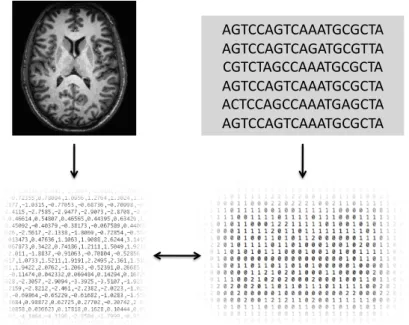
Neuroimaging genetic analysis involves the search for genomic variants, for example SNPs or copy number variations, associated with quantitative measures derived from brain scans (Figure 1.5). Typical neuroimaging-derived quantitative measures include those de-scribing the distribution of tissue types such as grey or white matter in the brain, variations in the size of anatomical structures such as cortical volume, or measures of brain connectiv-ity (Thompson, Martin, and Wright, 2010). The search for significant associations however presents a particular statistical challenge, due to the very high dimensionality of both geno-type and imaging data (Poline et al., 2010). For example, an imaging genetic study may in-volve a search for causal genetic associations between upwards of 500,000 SNPs and more than 100,000 voxels1_{. The simplest approach is one of ‘mass univariate linear modelling’}

(MULM), in which each genetic predictor is tested for association against each voxel-wise phenotype (see Figure 1.6, left). However, this approach has a number of drawbacks.

1_{Strictly speaking, the word voxel describes a single 3D picture element in a neuroimaging scan. We use}

the term interchangeably to describe any voxel-wise quantity (phenotype) derived from such an image. For example a scalar quantity measuring grey matter intensity or change in brain volume at a single voxel.

(29)

1.3 Imaging genetics 18 !"#$$!"#$!!!#"$"$#!% !"#$$!"#$!"!#"$"##!% $"#$#!"$$!!!#"$"$#!% !"#$$!"#$!!!#"$"$#!% !$#$$!"$$!!!#"!"$#!% !"#$$!"#$!!!#"$"$#!%

Figure 1.5: Imaging genetic analysis. Neuroimages, for example from MRI scans (top left), are used to derive quantitative measures describing features in the brain such as grey matter volume (bottom right). These are compared with measures of genomic variation, such as variations in SNP minor allele dosage (bottom right), obtained from candidate gene or genome-wide scans (top right).

Firstly, the potentially huge number of hypotheses tested under a MULM framework re-quires the application of a very large multiple testing correction, leading to a corresponding loss of power. Many imaging genetic studies reduce the scale of this problem by decreasing the number of tested hypotheses. This can be achieved for example by narrowing the search to a set of candidate genes (Hariri et al., 2002); focusing on specific ‘regions of interest’ (ROIs) obtained by parcelling the brain into different anatomical areas (Joyner et al., 2009); or modelling single imaging measures, derived for example by taking an average intensity value across a specific ROI (Potkin et al., 2009b). Each of these strategies involves either additional assumptions about putative associations, or the discarding of potentially infor-mative data. In contrast, a ‘hypothesis-free’ approach was taken by Stein et al. (2010b), who conducted the first brain-wide, genome-wide imaging genetics study in an investi-gation of SNPs associated with changes in brain structure in patients with Alzheimer’s Disease. To reduce the potentially huge amount of tested hypotheses (1010 voxel x SNP comparisons), only the most significant SNP at each voxel was assessed, combined with

(30)

an adjustment to the multiple testing threshold to account for dependencies between SNPs. This latter adjustment follows from the fact that correlation between SNPs arising from the LD structure present in genotype data means that voxel x SNP tests are not strictly inde-pendent. The effective number of tests is therefore reduced, so that a Bonferroni-corrected threshold is likely to be over conservative. In the genetic domain, such adjustments are well established (Johnson et al., 2010). Similar adjustments accounting for voxel-voxel depen-dencies arising from spatial correlations in the imaging domain have also been developed (Worsley, 2003), and these are discussed further in Chapter 6.

Aside from the multiple testing problem, a second potential drawback of the MULM approach is that by treating both gene variants and voxel-wise phenotypes as independent, the inherent structure in both is ignored. With genotypes, this structure may manifest as complex patterns of LD, or from functional associations of SNPs in genes and pathways, as discussed previously. With phenotypes, structure may arise from correlations between brain regions sharing structural and/or functional features, and there is evidence that many such features are under strong genetic influence (Peper et al., 2007; Chiang et al., 2009). As with the case of genotypes discussed previously (Section 1.1), the fact that multiple phenotypes may be influenced by many of the same genetic factors means that their joint modelling can be expected to boost power (Hibar et al., 2011a; Vounou et al., 2011).

Most multilocus approaches in imaging genetics involve either the modelling of a sin-gle summary phenotypic measure, or the performing of multiple independent multilocus tests of association against multiple phenotypes. For example, Bralten et al. (2011) used a multilocus, gene-based test of association to investigate the influence of the SORL1gene on hippocampal volume. Multiple linear regression models for the joint modelling of SNPs have also been employed. Problems of multicollinearity with genome-wide SNP data mean that this is often combined with some form of dimensionality reduction on the SNP data, for example using PCA to obtain orthogonal sets of predictors (Hibar et al., 2011b). This approach has the potential disadvantage of making the results of any such analysis diffi-cult to interpret or replicate, since any genetic factors identified then consist of principal components summarising the effect of multiple predictors. As discussed previously, sparse regression techniques offer an alternative solution. Penalised regression models applied to genotype estimation for the modelling of imaging-derived univariate phenotypes include

(31)

1.3 Imaging genetics 20

the use of ridge regression (Kohannim et al., 2011), the lasso (Kohannim et al., 2012a) and the elastic net (Kohannim et al., 2012b), with the first reporting a boost in power compared to a univariate analysis in which each SNP is considered separately.

A number of methods that are able to jointly consider genotypes and multivariate phe-notypes in a single multivariate model have been proposed. For example, multivariate latent variable models such as canonical correlation analysis (CCA), parallel independent component analysis (pICA) and partial least squares (PLS) have been used in an attempt to identify latent factors that capture some of the relationship between genetic and phe-notypic domains. CCA and pICA attempt to identify orthogonal (CCA) or independent (pICA) latent factors – specifically linear combinations of variables from each domain – that maximise the correlation between imaging and genetic data. Similarly, PLS identi-fies orthogonal latent factors that maximise between-domain covariance. These methods have been applied to the analysis of imaging genetic data (Hardoon et al., 2009; Calhoun, Liu, and Adali, 2009; Liu et al., 2009; Jagannathan et al., 2010). Studies so far conducted have used relatively small pools of SNPs and voxels, and concerns have been raised that the power to identify latent factors may be substantially reduced with genome-wide data (Hibar et al., 2011a). In addition, as with PCA, these latent variable models identify linear combinations of predictors (SNPs or voxels), making it hard to assess the importance of in-dividual predictors or compare results across studies (Hibar et al., 2011a; Vounou, Nichols, and Montana, 2010).

Recently, variations on some of these multivariate latent variable models have been introduced that enforce sparse selection of variables within latent factors. These mod-els, such as sparse CCA (Parkhomenko, Tritchler, and Beyene, 2009; Witten, Tibshirani, and Hastie, 2009; Chen and Liu, 2011) and sparse PLS (Chun and Kele, 2010) have re-cently been compared in an imaging genetic context (Le Flochcor et al., 2012). A closely related model, sparse reduced-rank regression (sRRR) (Vounou, Nichols, and Montana, 2010) builds on a previous technique in multivariate regression known as reduced-rank re-gression (Izenman, 2008), and identifies latent factors linking genotype and phenotype pre-dictors by constraining the rank of the matrix of estimated regression coefficients. sRRR imposes an additional regularisation penalty on the resulting coefficient estimates, for ex-ample using a lasso penalty, that enforces sparse solutions. In extensive simulations using

(32)

realistic imaging and genotypic data, sRRR demonstrated increased power to detect true genotype-phenotype associations, compared with a MULM approach (Vounou, Nichols, and Montana, 2010).

In Chapter 3, we describe a method that extends the P-GLAW method for pathways se-lection described in Chapter 2 to accommodate a multivariate quantitative phenotype. Our proposed ‘Pathways sparse Reduced-Rank Regression’ (PsRRR) model builds on the sRRR model, but performs pathway selection through the imposition of a group lasso penalty on genotype coefficients. We demonstrate proof of principle of the efficacy of our proposed method in simulation studies, and conclude Chapter 3 with an investigation of pathways associated with longitudinal structural change in Alzheimer’s disease, using a multivariate imaging phenotype.

1.3.1

Cluster size inference

Despite recent interest in multivariate methods, MULM remains the most common ap-proach to imaging genetics analysis. MULM techniques are also used widely for the map-ping of human brain function, for example in analysing fMRI to identify areas of height-ened activation during task-related activities (Ashburner et al., 2006). The primary output of a MULM analysis is then a list of test statistics, describing the extent of association be-tween each SNP or task at each voxel. These are often displayed as a statistical map (see Figure 1.6, middle and right).

The structural and functional architecture of the brain means that association signals may often extend across neighbouring voxels to form clusters of heightened activation. For this reason, statistical tests based on contiguous regions of heightened activation have been developed. These can offer increased power over voxel-wise tests, where for example ac-tivation at each voxel in a cluster does not on its own achieve statistical significance, but inference based on cluster-wise activation does (Poline et al., 1997). Cluster size inference works by first thresholding the statistical image at a particular significance level, and then comparing the size of any resulting super-threshold clusters with that expected by chance using random field theory (RFT) (Friston et al., 1996). Since the number of clusters is typically much smaller than the number of voxels, this method has the advantage of

(33)

requir-1.4 Mathematical notation and nomenclature 22 é0.5 0 0.5 1 1.5 2 2.5 é0.1 é0.08 é0.06 é0.04 é0.02 0 0.02 0.04 0.06 0.08 0.1 rs9681213 allele count intensity at [8, é 12, é 4] fitted plus error

Figure 1.6: MULM in imaging genetic analysis. Left: Association between activation at a single voxel (at location [8, -12, -4]) and minor allele count at a single SNP (RS9681213). Middle and right: Statistical maps (t-images) mapping the significance of the slope at each voxel across the brain. Sagittal (sideways) and coronal (front - on) sections are displayed.

ing a less stringent multiple testing correction, although this comes at the cost of reduced localising power.

With voxel-wise tests, the very large number of tests performed raises concerns about the adequate control of false positives (Meyer-Lindenberg et al., 2008). These concerns apply equally to cluster-size inference. In particular, the use of RFT to estimate the distri-bution of cluster sizes under the null rests on a number of assumptions, and these need to be verified empirically (Hayasaka and Nichols, 2003). In Chapter 6, we investigate the control of false positives using cluster size inference in an imaging genetics context, and find that a number of conditions with regard to cluster forming thresholds and image smoothness need to be met, if adequate control of type-I errors is to be guaranteed.

1.4

Mathematical notation and nomenclature

Throughout this thesis we use the terms predictor, genotype, genetic variant and SNP (sin-gle nucleotide polymorphism) interchangeably. Likewise for the terms quantitative trait, response and phenotype, and the terms pathway and group.

We assume all observations of genotypes and phenotypes are from a random sample of N unrelated individuals, drawn from the same population. Matrices are denoted by bold capital letters, and vectors by bold lower case. We additionally adopt the following notation for observed genotypes and phenotypes, and for gene pathways:

(34)

Genotypes

We assume that minor allele counts atP SNPs,x1, . . . , xP, are recorded forN subjects

and denote by xij ∈ {0,1,2}, the observed minor allele count for SNPj on individuali.

These observed minor allele counts are arranged in an(N _×P)SNP genotype matrix,X. We denote byxj = (x1j, . . . , xN j)0, the column vector of minor allele counts

correspond-ing to SNP j, so that X = (x1, . . . ,xP), and byxi. = (xi1, . . . , xiN)the vector of minor

allele counts corresponding to theith row ofX.

Phenotypes

We assume N observations of aQ-dimensional multivariate quantitative trait or phe-notype, y1, . . . , yQ. The observed values for phenotype q are arranged in an (N × 1)

column vector, yq, and the Q phenotypes are arranged in an (N ×Q) phenotype matrix

Y = (y1, . . . ,yQ). In the case thatQ = 1, we drop the subscript and denote the vector of

observations for the corresponding univariate phenotypeybyy.

Pathways

We frequently assume that SNPs may be mapped toLgroups or gene pathways,_Gl ⊂

{1, . . . , P_}, l = 1, . . . , L, using prior information extracted from a pathways database. We denote byPl, the number of SNPs in groupGl. Groups are sometimes assumed to be

disjoint, so that_Gl∩ Gl0 =∅for anyl 6=l0. We state clearly where this is or is not the case. For simplicity, in the text (but not in equations) we occasionally refer to ‘pathway l’, by which we mean the pathway indexed byl, that is_Gl.

For convenience, we index the SNPs in group _Gl byl1, . . . , lPl, while noting that each

index has a unique one-to-one mapping to the original set of SNP indices, so that lz ∈

{1, . . . , P_}forz = 1, . . . , Pl. We denote byXl = (xl1, . . . ,xl_Pl)the(N ×Pl)matrix of

minor allele counts corresponding to SNPs in pathway_Gl.

Throughout the text, we denote the cardinality, or number of elements in a set _S, by

|S|. Finally we denote the`qnorm of a p-dimensional vectorvas||v||q = (Pp_j₌₁|vj|q)

1 q_,

(35)

1.5 Abbreviations 24

1.5

Abbreviations

BCGD block coordinate gradient descent CGD coordinate gradient descent FDR false discovery rate

(f)MRI (functional) magnetic resonance imaging FWER family-wise error rate

FWHM full-width at half-maximum

GL group lasso

GWAS genome-wide association study/studies

LD linkage disequilibrium

MAF minor allele frequency

MC Monte Carlo

MLR multiple linear regression

MULM mass univariate linear modelling OLS ordinary least squares

PCA principal component analysis PET positron emission tomography

P-GLAW pathways group lasso with adaptive weights PGAS pathways gene association study/studies

P-SGLAW pathways sparse group lasso with adaptive weights PsRRR pathways sparse reduced-rank regression

QTL quantitative trait locus/loci QTT quantitative trait test ROI region of interest

RFT random field theory

SGL sparse group lasso

SGL-CGD sparse group lasso - coordinate gradient descent SNP single nucleotide polymorphism

sRRR sparse reduced-rank regression

(36)

Chapter 2

Identifying pathways associated with a

univariate quantitative trait: ‘Pathways

Group Lasso with Adaptive Weights’

We now turn to the problem of developing a multiple regression model for the identification of biological pathways associated with a quantitative trait. As outlined in Section 1.2, our assumption is that where causal SNPs are enriched in a pathway, an approach that includes all SNPs in a single, sparse multiple regression model will have increased power, compared to a more conventional approach in which SNPs are considered one at a time. To this end, we use a modified version of a sparse regression model known as the group lasso (GL) with SNPs grouped into pathways. We believe this is the first method able to jointly model the genome-wide, group-wise association of gene variants with a quantitative trait.

We face a number of challenges in applying GL to SNP and pathway data for the iden-tification of implicated pathways. These include the fact that pathways overlap, since many SNPs map to multiple pathways; the problem of selection bias, that is the tendency of the model to select pathways having specific statistical properties irrespective of their asso-ciation with the phenotype; and the problem of assessing pathway importance in a finite sample. In addition, the potentially very large size of SNP datasets makes the develop-ment of strategies for computationally efficient model estimation a necessity. In following sections we outline our approach to tackling each of these challenges.

(37)

2.1 Penalised regression approaches in gene mapping 26

The chapter is arranged as follows. We begin in Section 2.1, with a review of the most common penalised regression models used in gene mapping – ridge regression and the lasso and variations thereof. In Section 2.2 we describe the group lasso model, and explain its relevance to the selection of pathways in PGAS. We also describe our strategy for dealing with the fact that pathways overlap. In Section 2.3, we describe an estimation algorithm for the GL with overlaps, along with a number of strategies we employ to speed up the estimation process for the large datasets in PGAS. In Section 2.4 we outline our approach to reducing potential bias in pathway selection using an adaptive weight tuning procedure, and in Section 2.5 we explain a method for ranking pathways in order of importance, using a subsampling procedure that exploits finite sample variability.

In Section 2.6, we evaluate our method, which we call ‘Pathways Group Lasso with Adaptive Weights’ (P-GLAW) in a simulation study, using real genetic and pathway data with quantitative phenotypes simulated under an additive genetic model. We feel the use of real genotype and pathway data is crucial, so as to capture the distributions of gene size and number within a pathway, together with the complex SNP LD patterns and overlaps between pathways, all of which may have a significant effect on pathway ranking perfor-mance. We consider a range of scenarios with different causal SNP distributions and effect sizes, and compare our method with a popular, existing PGAS method based on combining multiple, univariate SNP-phenotype association statistics. To our knowledge, this is the first such power study comparing multivariate and univariate approaches using real SNP and pathway data. We conclude the chapter with a discussion in Section 2.7.

2.1

Penalised regression approaches in gene mapping

We return here to the problem, introduced in section 1.1, of estimating P SNP regression coefficients associated with a univariate, quantitative trait in a multiple linear regression model. In what follows, we assume that the response vector, y is mean-centred, so that

PN

i=1yi = 0. We additionally assume that the observed SNP allele count vectors are

mean-centred and of unit length, so thatPN

i=1xij = 0and

PN

i=1x 2

(38)

The standard, multiple linear regression model is given by

y=Xβ+,

where the errors, i, i = 1, . . . , N are assumed to be independent and identically

dis-tributed, with variance σ2_{. When the design matrix,} _{X, is of full rank, an unbiased}

es-timate for the regression coefficient vector, βis obtained by minimising the residual sum of squares_||y₋Xβ_||2 2 to give ˆ βOLS = (X0X)−1X0y (2.1) with variance Var( ˆβOLS) =σ2(X0X)−1.

Two problems immediately arise in the context of gene mapping. Firstly, multicollinear-ity due to LD between SNP predictors can make the inverse(X0X)−1very sensitive to small changes in the data. This makes the resulting estimates for individual SNP coefficients unreliable, undermining the original goal of identifying predictors with functional signif-icance (Malo, Libiger, and Schork, 2008). Secondly, in gene mapping we are frequently faced with the situation where there are more predictors than subjects. In this case X is rank deficient,X0Xis not invertible, and no unique estimates forβexist.

One possible solution is to take a model selection approach, in which we attempt to pick a subset of SNPs that best predicts the response. This strategy is used in a number of stepwise variable selection methods in which subsets of predictors are successively either included or excluded from the model, depending on their effect on the model’s goodness of fit. The discrete nature of these approaches however makes them unreliable, since at each step the model is optimised for a subset of predictors only. More exhaustive model selec-tion methods such asall subsets regressionalso suffer from bias, and are computationally feasible only for relatively small numbers of predictors (Hesterberg et al., 2008).

In contrast, continuous shrinkage or penalised regression methods have been shown to provide more reliable coefficient estimates than the discrete methods described above (Hastie, Tibshirani, and Friedman, 2008). These methods work by adding some form of

(39)

regularisation to the estimation ofβ. This typically involves the imposition of a constraint or penalty onβ, so that ˆ β = arg min β || y₋Xβ||2 2 subject to P(β)< c (2.2)

where the penalty functionP(β)is some function of the regression coefficients, andc >0. An equivalent expression is ˆ β = arg min β n ||y₋Xβ_||2 2+λP(β) o (2.3)

with λ > 0, where λ is a tunable parameter controlling the amount of regularisation or penalisation to be applied. Note there is a one-to-one correspondence between c and λ (Hastie, Tibshirani, and Friedman, 2008).

A common choice forP(β)is a function of the`γ-norm of the coefficient vectors,

P(β) =_||β_||γ γ = P X j=1 |βj|γ (2.4)

whereγ >0. Depending on the choice ofγ, the resulting estimates for the SNP coefficients exhibit some potentially useful properties. Moreover, withγ _≥1, the penalty (2.4) has the attractive property of being convex (strictly convex whenγ > 1), and as we shall see, this makes the resulting convex optimisation problem (2.3) amenable to efficient solutions.

We now consider the two paradigm cases in penalised regression, withγ = 1andγ = 2.

2.1.1

Ridge regression

The case with γ = 2is known asridge regression (Hoerl and Kennard, 1970). The ridge estimator (2.2) forβthen satisfies

ˆ

βridge _{= arg min}

β || y₋Xβ_||2 2 subject to P X j=1 β_j2 < c (2.5)

(40)

To better understand some of the properties of the ridge estimator, we begin by consider-ing the simple case of two predictors. The optimisation (2.5) then has a simple geometric interpretation, illustrated in Fig. 2.1. In the figure, dashed lines represent lines of increas-ing sum of squared residual error, _||y₋Xβ||2

2 asβˆmoves away from its optimum value

ˆ

βOLS _{= arg min}

β||y−Xβ||22. The ridge penalty ensures thatβˆridge is constrained to lie

within the region bounded by the blue circle,β2

1 +β22 = c. Estimates forβˆ

ridge

1 andβˆ

ridge

2

satisfying (2.5) then correspond to the blue point in Fig. 2.1. The effect of the ridge penalty is thus to shrink coefficient estimates, compared to their OLS values, with the amount of shrinkage increasing with decreasingc (or equivalently increasing λ). This shrinkage property can be very useful in the case of correlated predictors. For example, where two predictors are highly correlated, OLS estimation can result in large variations in estimated coefficients, where a large positive coefficient for one predictor is cancelled by a simi-larly large negative coefficient for the other. Such variations are constrained by the ridge penalty, which exhibits a ‘grouping effect’ that ensures correlated predictors have similar coefficients, potentially making results easier to interpret. This shrinkage property can also lead to superior prediction accuracy through a bias-variance trade off (Hastie, Tibshirani, and Friedman, 2008; Malo, Libiger, and Schork, 2008).

An equivalent form for the ridge optimisation (2.5) is

ˆ

βridge = arg min

β n ||y₋Xβ||2 2+λ P X j=1 β_j2o with solution ˆ βridge = (X0X+λI)−1X0y (2.6) whereIis the(P _×P)identity matrix. By comparing (2.6) with (2.1), we see how ridge regression enables the estimation of coefficients in theP > N case, whereXis rank defi-cient, since the addition of a positive constant to the diagonal ofX0Xrenders the problem non-singular, even whenX0Xis not of full rank (Hastie, Tibshirani, and Friedman, 2008).

Several recent studies have exploited properties of the ridge estimator highlighted above in the identification of important SNPs in GWAS, including in an imaging genetics context (Sun et al., 2009; Kohannim et al., 2011).

(41)

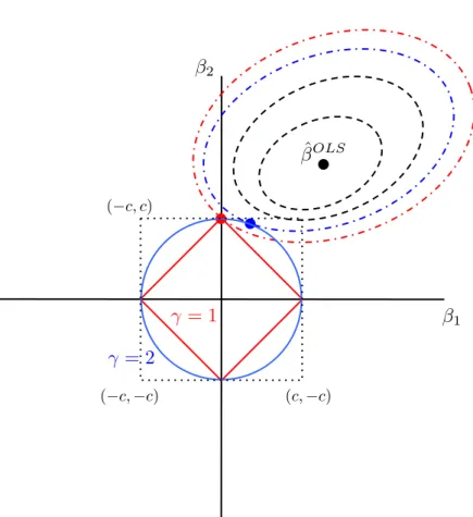
2.1 Penalised regression approaches in gene mapping 30 β1 β2 ˆ βOLS γ = 1 γ = 2 (c,₋c) (₋c,₋c) (−c, c)

Figure 2.1: Coefficient estimation with two predictors,β1andβ2. Dashed lines represent contours

of constant sum of squared residual error, ||y−Xβ||2

2. With ridge regression, the constraint is

β2

1 +β22 < c(blue circle) and the estimated coefficientsβˆridge correspond to the blue dot. With

lasso regression, the constraint is|β1|+|β2|< c(red diamond) and the estimated coefficientsβˆlasso

(42)

2.1.2

Variable selection with the lasso

The case withγ = 1is known aslasso regression(Tibshirani, 1996). The lasso estimator forβsatisfies

ˆ

βlasso _{= arg min}

β || y₋Xβ_||2 2 subject to P X j=1 |βj|< c. (2.7)

Once again considering the simple case with two predictors illustrated in Fig. 2.1, with the lassoβis constrained to lie within the region bounded by the red diamond,_|β1|+|β2|=c.

Estimates for βˆ₁lasso and βˆ₂lasso then correspond to the red point in Fig. 2.1. We see that ascapproaches zero (or equivalently λ moves away from zero), the contours of the OLS estimation are increasingly likely to intersect the red diamond at one of the axes, meaning that one of the coefficients, β1 or β2 is set to zero. The lasso thus performs a form of

variable or model selection, in the sense that a single variable is ‘selected’ by the model. This example readily extends to the P > 2 case, with the lasso producing sparse es-timates for βˆlasso_{, in the sense that multiple predictors have their coefficients,} _β_ˆlasso

j , set

to zero. The degree of sparsity is controlled bycorλ, such that an increasing number of predictors have zero coefficients as c is reduced, or equivalently λ is increased. We can then think of the lasso as selecting a subset of predictors,_Sˆ=_{j :βj 6= 0, j = 1, . . . , P}.

In high-dimensional, large P settings typical encountered in GWAS and gene expres-sion analysis, variable selection methods using penalised regresexpres-sion are attractive for a number of reasons. Firstly, a parsimonious model that selects a small number of impor-tant predictors is easier to interpret. In any case, in SNP mapping, we expect only a small set, _{S ⊂ {}1, . . . , P_}, of all predictors to be truly associated with the phenotype, so that the assumptions underlying sparse models such as the lasso are likely to hold. Secondly, as with ridge regression, the shrinkage property can improve a model’s capacity to pre-dict outcomes with new data, reducing variance at the expense of slightly increased bias (Hastie, Tibshirani, and Friedman, 2008). Finally, in contrast to the discrete subset selec-tion methods described previously, penalised regression models such as the lasso perform

continuousvariable selection, and thus tend to select the set of true predictors with greater

(43)

An important issue with all penalised regression models is the need to choose a value for the regularisation parameter, λ. For sparse regression models such as the lasso this determines the number of variables selected by the model. A common strategy is to use K-fold cross validation to choose a λ value that minimises the prediction error between training and test datasets. One drawback of this approach is that it focuses on optimising the size of the set, _Sˆ, of selected variables that minimises the cross validated prediction error. Since the variables in_Sˆwill vary across each fold of the cross validation, this proce-dure may not be a good means of establishing the importance of a unique set of variables (Vounou et al., 2011). Other approaches include the use of information-theoretic metrics such as the Akaike or Bayesian information criteria (AIC and BIC), that trade model good-ness of fit against model complexity (degrees of freedom) (Zou, Hastie, and Tibshirani, 2007). Data resampling or bootstrapping techniques have also been demonstrated to im-prov