Tensor completion via a multi-linear low-n-rank factorization model
Huachun Tan
a,n, Bin Cheng
a, Wuhong Wang
a, Yu-Jin Zhang
b, Bin Ran
ca
Department of Transportation Engineering, Beijing Institute of Technology, Beijing 100081, PR China b
Department of Electronic Engineering, Tsinghua University, Beijing 100084, PR China
cDepartment of Civil and Environmental Engineering, University of Wisconsin-Madison, 1415 Engineering Drive, Madison, WI 53706, USA
a r t i c l e i n f o
Article history:Received 19 April 2013 Received in revised form 15 September 2013 Accepted 18 November 2013 Communicated by Tao Mei Available online 20 January 2014
Keywords:
Tensor completion
Multi-linear low-n-rank factorization Nonlinear Gauss–Seidal method Singular value decomposition
a b s t r a c t
The tensor completion problem is to recover a low-n-rank tensor from a subset of its entries. The main solution strategy has been based on the extensions of trace norm for the minimization of tensor rank via convex optimization. This strategy bears the computational cost required by the singular value decomposition (SVD) which becomes increasingly expensive as the size of the underlying tensor increase. In order to reduce the computational cost, we propose a multi-linear low-n-rank factorization model and apply the nonlinear Gauss–Seidal method that only requires solving a linear least squares problem per iteration to solve this model. Numerical results show that the proposed algorithm can reliably solve a wide range of problems at least several times faster than the trace norm minimization algorithm.
& 2014 The Authors. Published by Elsevier B.V.
1. Introduction
A tensor is a multidimensional array which is the higher-order generalization of vector and matrix. It has many applications in information science, computer vision and graph analysis[1]. In the real world, the size and the amount of redundancy of the data increase fast, and nearly all of the existing high-dimensional real world data either have the natural form of tensor (e.g. multi-channel images and videos) or can be grouped into the form of tensor (e.g. tensor face[2]). Therefore, challenges come up in many areas when one confronts with the high-dimensional real world data. Tensor decomposition is a popular tool for high-dimensional data processing, analysis and visualization. Two particular tensor decomposition methods can be considered as higher-order exten-sions of the matrix singular value decomposition: CANDECOMP/ PARAFAC (CP) [3,4] and the Tucker [5]. Tensor decomposition gives a concise representation of the underlying structure of tensor, revealing when the tensor data can be modeled as lying close to a low-dimensional subspace. Although useful, they are not as powerful. For general tensors, tensor decomposition does
not deliver best low rank approximation, which will limit its applications.
In this paper, we will try to recover a low-n-rank tensor from a subset of its entries. This problem is called the tensor completion problem. It is also called missing value estimation problem of tensors. The problem in computer vision and graphics is known as image and video in-painting problem[6,7]. The key factor to solve this problem is how to build up the relationship between the known elements and the unknown ones. Owing to this reason, the algorithms for completing tensors can be coarsely divided into local algorithms and global algorithms. Local algorithms [8,9] assume that the further apart two points are, the smaller their dependence is and the missing entries mainly depend on their neighbors. Thus, the local algorithms can only exploit the informa-tion of the adjacent entries. However, sometimes the values of the missing entries depend on the entries which are far away and the local algorithms cannot take advantage of a global property of tensors. Therefore, in order to utilize the information of tensors as much as possible, it is necessary to develop global algorithms that can directly capture the complete information of tensors to solve the tensor completion problem.
In the two-dimensional case, i.e. the matrix, the rank is a powerful tool to capture the global information and can be directly determined. But for the high-dimensional case, i.e. the tensor, there is no polynomial algorithm to determine the rank of a specific given tensor. Recently, based on the extensions of trace norm for the minimization of tensor rank, some global algorithms [6,7,10–12] solving the tensor completion problem via convex optimization have been proposed. Liu et al.[6]first proposed the Contents lists available atScienceDirect
journal homepage:www.elsevier.com/locate/neucom
Neurocomputing
0925-2312 & 2014 The Authors. Published by Elsevier B.V. http://dx.doi.org/10.1016/j.neucom.2013.11.020
nCorresponding author. Tel./fax:þ86 10 68914582.
E-mail addresses:[email protected],[email protected](H. Tan),
[email protected](B. Cheng),[email protected](W. Wang),
[email protected](Y.-J. Zhang),[email protected](B. Ran).
Open access under CC BY-NC-ND license.
definition of the trace norm of an n-mode tensor as jjXjjn¼
ð1=nÞ∑n
i¼1jjXðiÞjjn. And similar to matrix completion, the tensor completion was formulated as a convex optimization problem. For tackling this problem, they developed a relaxation technique to separate the dependant relationships and used the block coordi-nate descent (BCD) method to achieve a globally optimal solution. The contribution of this paper is realized at the methodological level by considering a more general kind of the tensor completion problem. By the extension of the concept of Shatten-q norm for matrix, Signoretto et al.[10]defined tensor Shatten-{p,q} norm, which is formulated asjjXjjp;q¼ ðð1=nÞ∑in¼1jjXðiÞjjpΣ;qÞ
1=pand con-sistent with that for matrix. Compared to the trace norm defined in[6], Shatten-{p,q} norm is a more general tensor norm and the trace norm of tensor can be seen as a special case of Shatten-{p,q} norm ðjjXjj1;1¼ ð1=nÞ∑ni¼1jjXðiÞjjΣ1;1¼ ð1=nÞ∑ni¼1jjXðiÞjjn¼ jjXnjjÞ. Though the general tensor Shatten-{p, q} norm was defined in this paper, they mainly focused on the special case trace norm of tensor in their algorithm. Similar to the above two works, Gandy et al.[7]used the n-rank of a tensor as sparsity measurement and tried tofind the tensor of lowest n-rank that satisfies some linear constraints. In their algorithm, the tensor completion was con-verted into a multi-linear convex optimization problem. Based on the Douglas–Rachford splitting technique [13,14] and the alter-nating direction method of multipliers [15], trace norm was introduced as the convex envelope of the n-rank and an efficient algorithm to solve the multi-linear convex optimization problem was proposed. In these trace norm based algorithms, they consider the tensor completion problem as recovering a low-n-rank tensor from a subset of its entries, that is,
minXAℝI1I2⋯IN 1 2jjXYjjF s:t: 1 N ∑ N i¼1jj XðiÞjjnrcYΩ¼ℳΩ ð1Þ
where X;Y;ℳ are n-mode tensors with identical size in each mode. The elements of ℳ in the set
Ω
are given, while the remaining elements are missing.XðiÞis the mode-iunfolding ofX. jjUjjn denotes the trace norm defined by the sum of all singular values of the matrix. On the other hand, Zhang et al.[16]exploited the recently proposed tensor-singular value decomposition (t-SVD)[17]that is a group theoretic framework to solve the tensor compression and recovery problem. Theyfirst constructed novel tensor-rank like measures to characterize informational and structural complexity of tensor.The core strategy of all these algorithms to achieve the optimal solution is the same as that they estimate the variables sequen-tially, followed by certain refinement in each iteration. Although the details of the solution procedure in each algorithm are different, unfortunately, the refinement in each iteration of all these algorithms requires computing singular value decomposi-tions(SVD) that a task is increasingly costly as the tensor size and n-ranks increase. It is therefore desirable to exploit an alternative algorithm more efficient in solving tensor completion problem.
In this paper, a new global algorithm for tensor completion called tensor completion via a multi-linear low-n-rank factoriza-tion model (TC-MLFM) is proposed. As the size and structure of each mode of the given tensor are not always the same (e.g. RGB images), the new algorithm combines n-ranks of each tensor mode by weighted parameters. However, the problem is that the func-tion is generally NP-hard and hard to approximate due to the non-convex optimization of rankðXðiÞÞ. To solve this problem, we use n-rank factorization optimization problem to substituterankðXðiÞÞ. The new function is solvable and considered as our model. With the new weighted objective model, the proposed algorithm can utilize the mode information of the tensor with choice. To solve this model, a minimization method based on the nonlinear Gauss– Seidal method[18]that only requires solving a linear least squares problem per iteration is applied. By adopting this method along
each mode of the tensor other than minimizing the trace norm in Eq. (1), the new algorithm can avoid the SVD computa-tional strategy and reliably solve a wide range of tensor comple-tion problems much faster than the trace norm minimizacomple-tion algorithm.
The rest of the paper is organized as follows.Section 2presents some notations and basic properties of tensors. Insection 3, we review the definition of Tucker decomposition and tensor n-rank, which suggests that a low-n-rank tensor is a low rank matrix when appropriately unfolded. Section 4 discusses the detailed process of the proposed algorithm.Section 5reports experimental results of our algorithm on simulated data and image completion. Finally,section 6provides some concluding remarks.
2. Notations and basics on tensors
In this paper, the nomenclatures and the notations in[1,19]on tensor are partially adopted. Scalars are denoted by lowercase letters (a,b,c,…), vectors by bold lowercase letters (a,b,c,…) and matrices by uppercase letters (A,B,C,…). Tensors are written as calligraphic lettersðA; ℬ;C;…Þ.
n-Mode tensors are denoted asAAℝI1I2⋯IN:Its elements are denoted as ai1…ik…iN, where 1rikrIK, 1rKrN. The mode-n unfolding (also called matricization or flattening) of a tensor AAℝI1I2⋯IN is defined as unf oldðA;nÞ ¼A
ðnÞ. The tensor ele-mentði1;i2;…;iNÞis mapped to the matrix elementðin;jÞ, where j¼1þ ∑N k¼1 kan ðik1ÞJk with Jk¼ ∏ k1 m¼1 man Im: ð2Þ Therefore,AðnÞAℝInJ, whereJ¼∏N kka¼1n
Ik. Accordingly, its inverse operator fold can be defined asf oldðAðnÞ;nÞ ¼A:
The n-rank of aN-dimensional tensorAAℝI1I2⋯IN, denoted byrn, is the rank of the mode-nunfolding matrixAðnÞ.
rn¼ranknðAÞ ¼rankðAðnÞÞ: ð3Þ
The inner product of two same-size tensorsA;ℬAℝI1I2⋯IN is defined as the sum of the products of their entries, i.e.
〈A;ℬ〉¼∑ i1 ∑ i2 ⋯∑ iN
ai1…ik…iNbi1…ik…iN: ð4Þ
The corresponding Frobenius norm isjjAFjj ¼pffiffiffiffiffiffiffiffiffiffiA;A. Besides, the
ℓ0norm of a tensorA, denoted byjjA0jj, is the number of non-zero elements in A and the ℓ1 norm is defined as jjA1jj ¼ ∑i1…ik…iNjai1…ik…iNj. It is clear that jjAjjF¼ jjAðnÞjjF, jjAjj0¼ jjAðnÞjj0 andjjAjj1¼ jjAðnÞjj1for any 1rnrN. Then-mode (matrix) product of a tensorAAℝI1I2⋯IN with a matrixMAℝJIn is denoted by AnM and is size I1⋯In1JInþ1⋯IN. In terms of
flattened matrix, then-mode product can be expressed as follows: Y¼AnM3YðnÞ¼MAðnÞ: ð5Þ
3. Tucker decomposition and low-n-rank tensor
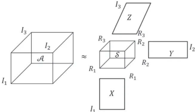
The Tucker decomposition[5]is a form of higher-order princi-pal component analysis. It decomposes a tensor into a core tensor multiplied (or transformed) by a matrix along each mode. Thus, in the three-way case whereAARI1I2I3, we have
AS1X2Y3Z: ð6Þ hereSAℝR1R2R3is called the core tensor and its entries show the level of interaction between the different components.XAℝI1R1, YAℝI2R2, ZAℝI3R3 are the factor matrices (which are usually orthogonal) and can be thought of as the principal components in
each mode. If R1;R2;R3 are significantly smaller than I1;I2;I3, respectively, the core tensorScan be thought of as a compressed version of A and then we consider A as a low-n-rank tensor. Formally, A is called low-n-rank tensor if its unfoldings are low-rank matrices. Thus we can use the ranks of unfoldings of a tensorAto learn low-n-rank tensorA. This rank should not be confused with the idea of tensor CP-rank [3,4]. An illustration of Tucker model for third-order tensors is given in Fig. 1. For notational simplicity, we illustrate our results in this paper using third order tensors, while generalizations to high order cases are straightforward.
4. Tc-MLFM
This section is separated into two parts. Part 1 extends the matrix completion problem to tensor case and converts the tensor comple-tion problem into a weighted multi-linear low-n-rank factorizacomple-tion model. Part 2 applies the nonlinear Gauss–Seidal method to solve the objective model and presents the details of solution procedure. 4.1. The factorization model of tensor completion problem
The derivation starts with the well-known optimization pro-blem for the low rank matrix completion[20,21]:
min :
LAℝmnrankðLÞ s:t: LΩ¼ MΩ; ð7Þ whererankðLÞdenotes the rank ofL, and the elements ofMin the set
Ω
are given while the remaining elements are missing. Eq.(7)aims to use a low rank matrixLto approximate the given matrix with missing elements. The optimization problem in Eq. (7) is a non-convex optimization problem since the functionrankðLÞis non-convex.The higher-order tensor completion problem can be generated from the matrix (i.e. 2nd-order tensor) case by utilizing the form of Eq.(7), leading to the following formulation:
min
ℒAℝI1I2⋯IN:rankCPðℒÞ s:t: ℒΩ¼ℳΩ; ð8Þ where the rank of ℒ denotes the CP-rank of tensor, ℒ;ℳ are n-mode tensors with identical size in each mode. The elements of ℳ in the set
Ω
are given while the remaining elements are missing.The definition of CP-rank, in the form of rankCPðXÞ, is the minimum number of rank-1 tensors that generateX as their sum [3,4]. In other words, CP-rank is the minimum number of compo-nents in an exact CP decomposition. The CP-rank of a tensor is defined as an exact analogue to the definition of matrix rank, but the properties of matrix are quite different from that of tensors. For instance, the CP-rank of a real-valued tensor may actually be different from mode to mode. One major difference between matrix rank and tensor CP-rank is that there is no straightforward algorithm to
determine the CP-rank of a specific given tensor. Therefore, Eq.(8) is difficult to solve. In fact, the problem is NP-hard[1,22].
On the other hand, the n-rank is defined as the dimension of the vector space spanned by the mode-n unfolding matrix. As discussed in Section 3, when the given tensor is a low-n-rank tensor, the n-ranks instead of the CP-rank of a tensor can be used to capture its global information. Therefore, we can minimize the n-ranks of the given tensor instead of minimizing the CP-rank to solve the tensor completion problem. As a result, a function F which minimizes the n-ranks of the given tensor to replace Eq.(8) is obtained as the following shows:
Fð min
ℒAℝI1I2⋯IN:ðrankðLð1ÞÞ;rankðLð2ÞÞ;…rankðLðNÞÞÞ s:t:ðLðiÞÞΩ¼ ðMðiÞÞΩ; ð9Þ whereLðiÞ;MðiÞare the mode-iunfoldings ofℒandℳ. As the size and structure of each mode of the given tensor are not always the same, the contribution of each mode to the final result may be different. Then the n-rank minimization problem of each mode can be combined by weighted parameters:
Fð min
ℒAℝI1I2⋯IN:ðrankðLð1ÞÞ;rankðLð2ÞÞ;…rankðLðNÞÞÞ
¼∑N i
λ
i minLðiÞrankðLðiÞÞ : ! :thus, the tensor completion problem becomes: ∑N i¼1
λ
i minLðiÞrankðLðiÞÞ : ! s:t:ðLðiÞÞΩ¼ ðMðiÞÞΩ: ð10ÞEq.(10)aims to find a low-n-rank tensorℒto approximate the given tensor with missing elements. A tensor is a multidimen-sional array or an element of the tensor product ofNvector spaces. That is to say matrix is special instance of tensor.
By comparing Eq.(10)to Eq.(7), we can observe that Eq.(10)is derived from the tensor completion problem and can be viewed as a weighted multi-linear matrix completion problem. In other words, matrix completion problem is also a special instance of tensor completion problem.
Although the elements involved in are all matrices, it is a highly non-convex optimization problem since the optimism function includes n-ranks. Without converts there is no efficient solution to this optimization problem[23]. In this paper, our goal isfinding a low-n-rank tensor ℒ so that jjðLðiÞÞΩðMðiÞÞΩjj2F (i¼1 to N ) is minimized. In fact, any matrix SAℝmn having a rank up to D can be expressed as a matrix multiplication S¼XY where XAℝmDandSAℝDn. In order to solve the function Eq. (10), additional auxiliary elenments ZðiÞ;XðiÞandYðiÞ will be introduced, while ZðiÞ¼XðiÞYðiÞ. To simplify the problem, we will minimize a F-norm instead of directly minimize the rank of the mode-i unfold-ings. Thus, Eq.(10)can be converted into the following form:
∑N i¼1
λ
i min XðiÞ;YðiÞ;LðiÞ 1 2jjZðiÞLðiÞjj 2 F : 0 B @ 1 C A; s:t: ZðiÞ¼XðiÞYðiÞ ðLðiÞÞΩ¼ ðMðiÞÞΩ: ð11ÞInstead of directly solving Eq.(11), we can solve the following problem:
ℋðXðiÞ;YðiÞ;LðiÞÞ ¼ min XðiÞ;YðiÞ;LðiÞ
1
2 XðiÞYðiÞLðiÞ 2 F; s:t: ðLðiÞÞΩ¼ ðMðiÞÞΩ for i¼1;2…N; respectively: ð12Þ
Y
4.2. Minimization via the nonlinear Gauss–Seidal method
The functionℋðXðiÞ;YðiÞ;LðiÞÞis differentiable and the gradient of the functionℋðXðiÞ;YðiÞ;LðiÞÞis shown as follows:
gradℋðXðiÞ;YðiÞ;LðiÞÞ ¼ ∂Xℱ ðiÞ; ∂ℱ YðiÞ; ∂ℱ LðiÞ
¼ ððXðiÞYðiÞLðiÞÞYðiÞT;XðiÞTðXðiÞYðiÞLðiÞÞ; XðiÞYðiÞLðiÞÞ;
s:t:ðLðiÞÞΩ¼ ðMðiÞÞΩ fori¼1;2…N;respectively: ð13Þ
Letð∂ℱ=Xð ÞiÞ ¼0;ð∂ℱ=YðiÞÞ ¼0;ð∂ℱ=LðiÞÞ ¼0, obtaining the optimal XðiÞ;YðiÞ;LðiÞ:
XðiÞ’LðiÞYðiÞTðYðiÞYðiÞTÞ1; YðiÞ’ðXðiÞXðiÞTÞ1XðiÞTLðiÞ;
LðiÞ’LðiÞYðiÞTðYðiÞYðiÞTÞ1ðXðiÞXðiÞTÞ1XðiÞTLðiÞ
þPΩðMðiÞXðiÞYðiÞÞ for i¼1;2…N; respectively: ð14Þ where AT is the transposed matrix of A. B1 denotes the Moore–Penrose pseudo-inverse matrix ofB that is a generaliza-tion of the inverse matrix. In linear algebra, BB1B¼B, B1BB1¼B1, ðBB1ÞT
¼BB1 andðB1BÞT
¼B1B. In Eq.(14), YðiÞTðYðiÞYðiÞTÞ1¼YðiÞ1andðXðiÞXðiÞTÞ1XðiÞT¼XðiÞ1. Thus, Eq.(14) can be formulated as follows:
XðiÞ’LðiÞYðiÞ1’LðiÞYðiÞTðYðiÞYðiÞTÞ1; YðiÞ’XðiÞ1LðiÞ’ðXðiÞXðiÞTÞ1XðiÞTLðiÞ; LðiÞ’LðiÞYðiÞ1XðiÞ1LðiÞþPΩðMðiÞXðiÞYðiÞÞ
for i¼1;2…N; respectively: ð15Þ
In [13], a sequence of lemmas have been derived. According to these lemma, orthðLðiÞYðiÞTÞ’LðiÞYðiÞT’LðiÞYðiÞ1, where orthðWÞ is an orthonormal basis for the range spaceRðWÞofW. Therefore, Eq.(15)can be converted into the following form:
XðiÞ’orthðLðiÞYðiÞTÞ’LðiÞYðiÞT’LðiÞYðiÞ1’LðiÞYðiÞTðYðiÞYðiÞTÞ1; YðiÞ’ðorthðLðiÞYðiÞT
ÞÞTL
ðiÞ’XðiÞ1LðiÞ’ðXðiÞXðiÞTÞ1XðiÞTLðiÞ; LðiÞ’orthðLðiÞYðiÞTÞðorthðLðiÞYðiÞTÞÞTþPΩðMðiÞXðiÞYðiÞÞ
for i¼1;2…N; respectively: ð16Þ
In order to optimize the algorithm, the nonlinear Gauss–Seidal method[18]can be competent. The optimized process starts with initializations. The core idea of this strategy is to optimize a group of variables while fixing the other groups. The variables in the optimization areXðiÞ,YðiÞand LðiÞ, which can be divided into three groups. To achieve the optimal solution, the method estimatesXðiÞ, YðiÞ andLðiÞ sequentially, followed by certain refinement in each iteration. The underlying optimization can be implemented using the initialization. The final solution is deduced by utilizing the result of each mode with the weighted parameters
λ
i in Eq.(11) given by the following:ℒ¼ ∑N i¼1
λ
iℒðiÞ= ∑ N i¼1λ
i ð17ÞThe pseudo-code of the TC-MLFM algorithm is given inTable 1 below.
5. Experiments
In this section, the performance of the proposed algorithm is evaluated and compared with LRTC (Low Rank Tensor Completion) [6] on both simulated data and real data. LRTC solves the optimization problem: minX;Y;ℳ ∑ N i¼1
λ
ijjMðiÞjjnþ ∑ N i¼1α
i 2jjXðiÞMðiÞjj 2 F þ ∑N i¼1β
i 2 YðiÞMðiÞ 2 F s:t: YΩ¼ℳΩ; ð18Þwhich is derived as the substitution to their original problem Eq.(1). The codes for our algorithm and LRTC both are implemen-ted under the Matlab environment. All the experiments are conducted and timed on the same desktop with an AMD Athlon (tm)4 640 Professor 3 GHZ CPU and 4 GB RAM.
A major challenge of our algorithm is the selection of para-meters and the initial values. In experiments, we simply set the parameters and the initial values as follows:
λ
¼ I1 SUMðIÞ; I2 SUMðIÞ;⋯ IN SUMðIÞ ;where SUMðIÞ ¼I1þI2þ⋯INUYð0iÞAℝDn¼eyeðD;nÞ is a diagonal matrix with one on the diagonal. L0ðiÞ¼MðiÞ, itermax¼500 andtol¼1:25104. The stop criterions of the proposed algo-rithm are defined as follows:
sc1¼jjPΩðMðiÞX k ðiÞYkðiÞÞjjF jjPΩðMðiÞÞjjF r tol and sc2¼ 1 jjPΩðMðiÞX k ðiÞYkðiÞÞjjF jjPΩðMðiÞXkði1Þ YkðiÞ 1ÞjjF rtol=2: ð19Þ 5.1. Numerical simulations
The tested low-n-rank tensors are created randomly by the following procedure. The N-way Tensor Toolbox [24]is used to generate a third order tensor with the size ofI1I2I3and the relative small n-rank of [r1r2r3]. The generated tensor is in Tucker model[5]described asℒ0¼A1X2Y3Z. To impose these rank conditions, A is a ℝr1r2r3 core tensor with each entry being sampled independently from a standard Gaussian distribution Nð0;1Þ,X;YandZ areI1r1,I2r2,I3r3factor matrices gen-erated by randomly choosing each entry fromNð0;1Þ. Here with-out loss of generality we make the factor matrices orthogonal. But one major difference is that the n-ranks are always different along each mode while the column rank and row rank of a matrix are equal to each other. For simplicity, in this paper, we set the n-ranks with the same value. Then a subset ofpentries was missing by a probability which follows a uniform distribution. The ratiop=∏n
iIi between the number of missing entries and the total number of entries in the tensor is denoted bymr(missing ratio). The values of missing entries are set to 0. In this section, the relative square error (RSE) toℒ0is used to measure the quality of recovery, which Table 1
The pseudo-code of TC-MLFM algorithm.
TC-MLFM: tensor completion via a multi-linear low-n-rank factorization model
Input:the observed dataℳAℝI1I2⋯IN;index setΩ.
Fori¼1to N
1: Unfoldℳalong each mode to get MðiÞ. 2: Initializations and Parameters:Y0
ðiÞAℝDn;L0ðiÞ¼MðiÞ;k¼0;λ¼ ½λ1λ2…λn: While not converged do
3: Xkþ1 ðiÞ ¼orthðLkðiÞðYkðiÞÞTÞ. 4: Ykþ1 ðiÞ ¼ ðorthðLkðiÞðYkðiÞÞTÞÞTLðiÞ. 5: Lkþ1 ðiÞ ¼XðkiÞþ1YkðiþÞ1þPΩðMðiÞXðkiþÞ1YkðiþÞ1Þ. 6: k¼kþ1. End while ℒðiÞ¼f oldiðLðiÞÞ. End for Output:ℒ¼∑N i¼1λiℒðiÞ=∑Ni¼1λi:
is defined as LRSE¼ jjℒ^ℒ0jjF=jjℒ0jjF, whereℒ^ is the recovered tensor from the tensor with missing entries.
Firstly, the ability of our algorithm in recovering low-n-rank tensors with missing elements is tested. We address this recover-ability issue by generating phase diagram and curve diagram in Figs. 2 and 3. The simulated tensors used in this test are of size 150150150 with the missing ratio mrchosen in the order as it appears in {0.05:0.05:0.95} and with each n-ranks value of {[555]:[222]:[494,949]}. In each case, TC-MLFM is run on 10 random instances. The phase diagram depicts the average value out of every 10 runs by our algorithm for each test case. A run was successful when the LRSE between the true and the recovered was smaller than 103. In Fig. 2, a white box indicates a successful recovery, while a black box means a failing recovery.Fig. 3 plots the average LRSE corresponding to the set of missing ratiomrwith different n-ranks, respectively. For all cases with different n-rank, the average LRSE increase gradually with the increase ofmr. That is to say if our algorithm recovers the random instance successfully formr¼
α
and n-rank ¼β
, then it ought to have equal or higher recoverability formroαand n-rank¼β
. Thus, it is concluded that TC-MLFM is particularly sensitive to the change ofmrfor this class of problems over a considerable range. Furthermore, under the condition offixed mr, it can be seen fromFig. 3that the smaller the n-rank, the smaller the LRSE minimum is.According to the above experiments, it is reasonable to infer that TC-MLFM is an acceptable algorithm to solve the low-n-rank tensor completion problem. However, an important question about the proposed algorithm is whether or not it is able to recover low-n-rank tensors similar to that of solving the trace norm minimization approach. Or simply put, does our algorithm provide a comparable recoverability to that of a good trace norm minimization algorithm? In the following part of this section, we will answer this question. Using numerical simulations, the proposed TC-MLFM algorithm is compared with LRTC algorithm [6]. The numerical simulated tensors used in our experiments are both of the same size and different size along each mode. A brief comparison of the two algorithms is presented inTables 2 and 3
(across 10 instances), where time denotes the CPU time measured in seconds and LRSE¼ jjℒ^ℒ0jjF=jjℒ0jjF denotes the relative square error between the true and the recovered tensors. From the data inTables 2 and 3, TC-MLFM algorithm is at least several times (often a few orders of magnitude) faster than the LRTC algorithm while the results of TC-MLFM are comparable to LRTC in terms of accuracy. Of course, the reported performances of the two solvers involved are pertinent to their tested versions under the specific testing environment. Improved performances are possible for different parameter settings, on different test problems, or by different versions. However, given the magnitude of the time between MLFM and LRTC, the advantage in speed of TC-MLFM should be more than evident on these test problems. 5.2. Image completion
In the above experiments, we tested the proposed algorithm on numerical simulations and compared it with LRTC. The numerical simulated experiments can be considered as low-n-rank tensor completion problems because the given samples are from a true low-n-rank tensor. In the following experiments, the proposed algorithm is applied on real data. The given samples of real data are taken from a tensor of mathematically full n-ranks. Therefore, the problem is considered as the low-n-rank approximation. The key difference between the two classes lies in whether a given sample is from a true low-n-rank tensor (with or without noise) or
n-rank missing ratio 10 20 30 40 50 0.1 0.2 0.3 0.4 0.5 0.6 0.7 0.8 0.9
Fig. 2.Phase diagram for low-n-rank tensor completion recoverability.
0 0.1 0.2 0.3 0.4 0.5 0.6 0.7 0.8 0.9 1 101 100 10-1 10-2 10-3 10-4 10-5 missing ratio LRSE n-rank=[5 5 5] n-rank=[13 13 13] n-rank=[23 23 23] n-rank=[33 33 33]
Fig. 3. Curve diagram for low-n-rank tensor completion recoverability.
Table 2
Correct recovery for random problems of the same size along each mode.
Problem TC-MLFM LRTC
Size n-Rank MR LRSE Time (s) LRSE Time (s)
100100100 [10 10 10] 0.1 6.1831e05 0.9376 0.0007 63.8986 [10 10 10] 0.3 9.1643e05 1.3219 0.0017 155.9281 [10 10 10] 0.5 0.0001 1.3438 0.0063 150.3079 [10 10 10] 0.7 0.0005 6.2641 0.0189 212.6063 [10 10 10] 0.9 0.2754 2.6907 0.7672 256.8374 [20 20 20] 0.1 8.4701e05 1.1108 0.0008 104.8659 [20 20 20] 0.3 0.0001 1.3266 0.0028 187.2174 [20 20 20] 0.5 0.0003 2.9876 0.1165 253.9469 [20 20 20] 0.7 0.0234 20.2515 0.4898 257.4905 [20 20 20] 0.9 0.8875 15.0235 0.9072 258.6530 [30 3030] 0.1 0.0001 1.5812 0.0015 93.2876 [30 30 30] 0.3 0.0002 2.1280 0.0107 95.3374 [30 3030] 0.5 0.0011 12.5842 0.0337 175.3766 [30 3030] 0.7 0.2558 17.8406 0.5636 256.5564 [30 30 30] 0.9 0.9836 2.3031 0.9296 73.3531 Table 3
Correct recovery for random problems of different size along each mode.
Problem TC-MLFM LRTC
Size n-Rank MR LRSE Time (s) LRSE Time (s)
80100120 [10 10 10] 0.1 5.3139e05 0.8157 0.0007 60.4376 [10 10 10] 0.3 9.8826e05 1.067 0.0018 147.3046 [10 10 10] 0.5 0.0001 1.0188 0.0064 141.4235 [10 10 10] 0.7 0.0015 2.7639 0.0194 201.2249 [10 10 10] 0.9 0.2639 12.5799 0.7679 250.9750 [20 20 20] 0.1 7.8343e05 1.0437 0.0008 100.4768 [20 20 20] 0.3 0.0001 1.1889 0.0029 182.9486 [20 20 20] 0.5 0.0003 1.6124 0.1129 246.9281 [20 20 20] 0.7 0.0449 15.9234 0.4718 251.1953 [20 20 20] 0.9 0.9262 7.5655 0.9058 252.0047 [30 3030] 0.1 0.0001 1.2516 0.0015 89.7077 [30 30 30] 0.3 0.0002 1.6001 0.0108 94.6763 [30 3030] 0.5 0.0103 4.6079 0.0341 176.7843 [30 3030] 0.7 0.3017 21.1204 0.5697 250.1733 [30 30 30] 0.9 0.9380 3.5455 0.9286 73.0626
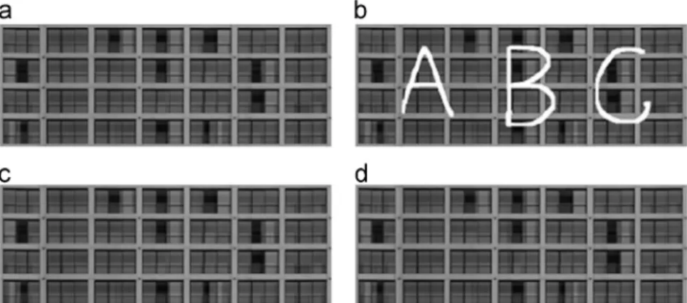
Fig. 4. Comparisons with LRTC on façade image: (a) the original image, (b) the original image with three uppercase letters as the missing parts shown in white, (c) the recovered image by TC-MLFM, and (d) the recovered image by LRTC.
Table 4
Comparisons of RSE and CPU time on façade image.
TC-MLFM LRTC
RSE Time RSE Time
0.0039 13.5630 0.0102 4701.2190
Fig. 5.Comparisons in terms of the natural image. Top row from left to right: the original image with 40%, 50%, 60% and 70% randomly missing entries, respectively. The second row from left to right: recovered image by TC-MLFM. The third row from left to right: recovered image by LRTC. The bottom: the original image.
not. In fact, low-n-rank approximation is more frequently used in practical applications.
One straightforward application of our algorithm is image completion. In this section, we outline the image completion examples with three different types of data: façade image, natural image and CT/MRI image. In the following tables, time denotes the CPU time measured in seconds and RSE¼ jjrecovered data
original datajjF=jjoriginal datajjF denotes the relative square error between the original data and recovered data.
Façade image: For façade image, we select three uppercase letters as the missing parts shown in white. The input data is a three-channel image and can be seen as a third-order tensor of dimensions 8613183.Fig. 4shows a recovery experiment of facade image: (a) is the original image, (b) is the input data, (c) is the recovered image by TC-MLFM, and (d) is the recovered image by LRTC.
Table 4 tabulates the RSE and CPU time of TC-MLFM and LRTC on façade image. From the data inTable 4, we can see that TC-MLFM algorithm is much faster than the LRTC algorithm while the results of TC-MLFM are comparable to LRTC in terms of accuracy.
Natural image: For natural image, the missing entries are ran-domly removed by different percentage and the ranran-domly removed pixels are shown in white. The input data is a three-channel image
and can be seen a third order tensor of dimensions 2562563. Fig. 5shows a recovery experiment of natural image. The top row of Fig. 5shows the original image with 40%, 50%, 60% and 70% randomly missing entries from left to right, respectively. The second row shows the recovered image by TC-MLFM. The third row shows the recov-ered image by LRTC. The bottom image is the original data.
Table 5tabulates the RSE and CPU time of TC-MLFM and LRTC on natural image. From the data in Table 5, it can be seen that TC-MLFM algorithm is at least several times faster than the LRTC algorithm while the results of accuracy are better than LRTC.
MRI image: In this part for the experiments we used MRI images, which contain 140 slices through a human brain, each having dimensions 217181. So the input data is a third-order tensor of dimensions 217181140. The missing entries were randomly removed with different percent and the randomly select pixels for removal are shown in white. Fig. 6 shows a recovery experiment offive slices in the MRI images. The top row shows the
five slices of the original data. The second row shows the original image with 50% randomly missing entries. The third row shows the recovered image by TC-MLFM. The bottom row shows the recovered image by LRTC.
Table 6 tabulates the RSE and CPU time of TC-MLFM and LRTC on MRI image. From the data in Table 6, it is observed that TC-MLFM algorithm is several times faster than the LRTC algorithm while the results of TC-MLFM are better than LRTC in terms of accuracy.
Table 5
Comparisons of RSE and CPU time on natural image.
MR TC-MLFM LRTC
RSE Time RSE Time
0.4 0.0598 3.1090 0.0837 53.0940
0.5 0.0748 2.6250 0.1083 64.4840
0.6 0.0954 1.9540 0.1392 77.8909
0.7 0.1219 2.2340 0.1799 99.4680
Fig. 6.Comparisons in terms of MRI image. The top row: thefive slices of the original data. The second row: the original image with 50% randomly missing entries. The third row: recovered image by TC-MLFM. The bottom row: recovered image by LRTC.
Table 6
Comparisons of RSE and CPU time on MRI image.
MR TC-MLFM LRTC
RSE Time RSE Time
5.3. Potential application
In the above, the proposed algorithm is applied to image comple-tion, such as façade image complecomple-tion, natural image complecomple-tion, and CT/MRI image completion. Besides image completion, may be the proposed algorithm can be used in other areas such as text mining, image classification, and video indexing. In [25], Dunlavy et al. analyzed data with multiple link types and derived feature vectors for each individual node. For the multiple linkages, a third order tensor was used, where each two-dimensional frontal slice represents the adjacency matrix for a single link type. Our algorithm is also a tensor based algorithm. The data used in[25]can be seen as a special case of our algorithm input. In[26], Zha et al. considered image classification as both a multi-label learning and multi-instance learning problem. Based on hidden conditional randomfields, they proposed an inte-grated multi-label multi-instance learning approach, which simulta-neously captures both the connections between semantic labels and regions. Thus, they formulated correlations among the labels in a single model. As is known that tensor is a useful tool for representing multi-mode correlations, and tensor decompositions facilitate a type of correlation analysis that incorporates all mode correlation simulta-neously. In[27], based on the optimum experimental design criteria in statistics, Zha et al. proposed a novel video indexing approach that makes use of labeled and unlabeled data and simultaneously exploits sample’s local structure, and sample relevance, density, and diversity information. In our knowledge, tensor also can formulate these elements into one model and mining the correlations between them simultaneously. And in the former work, we have applied tensor recovery into background modeling using video data[28]and traffic data completion[29]. In the future, we will investigate the applications of our algorithm to these areas.
6. Conclusion
In this paper, we extend the low-rank matrix completion problem to a low-n-rank tensor completion problem and propose an efficient algorithm based on the multi-linear low-n-rank factorization model. For the solution of this model, the nonlinear Gauss–Seidal method that only requires solving a linear least squares problem per iteration is applied. Thus, the proposed algorithm can avoid the singular value decompositions (SVD) strategy which is much time cost. And the proposed algorithm can automatically complete a low-n-rank tensor with missing entries. The performance of the proposed algorithm is evaluated on both simulated data and real data. The experiments show that the proposed algorithm is much less computational cost than the trace norm minimization algorithm especially facing the large data. Different applications in image completion show the applicability of our proposed algorithm in the real world data.
In the future, we would like to investigate how to automatically choose the optimal weighted parameters in our algorithm and develop more efficient algorithm for tensor completion problem. Also we will explore additional applications of our method in the real world data.
Acknowledgment
This work was supported by National Natural Science Founda-tion of China (61271376, 61171118, 91120010), NaFounda-tional Basic Research Program of China (973 Program: no. 2012CB725405), and Beijing Natural Science Foundation (4122067). We would like to thank Ji Liu from University of Wisconsin-Madison to improve the manuscript. The authors would like to thank experienced anonymous reviewers for their constructive and valuable sugges-tions for improving the overall quality of this paper.
References
[1]T.G. Kolda, B.W. Bader, Tensor decompositions and applications, SIAM Rev.
51 (3) (2009) 455–500.
[2] M.A.O. Vasilescu, D. Terzopoulos, Multilinear analysis of image ensembles: tensor faces, in: European Conference on Computer Vision (ECCV), 2002, pp. 447–460. [3]J.D. Carroll, J.J. Chang, Analysis of individual differences in multidimensional
scaling via an N-way generalization of Eckart–Young decomposition,
Psycho-metrika 35 (1970) 283–319.
[4] R.A. Harshman, Foundations of the PARAFAC Procedure: Models and Condi-tions for an“Explanatory”Multi-modal Factor Analysis, UCLA Working Papers in Phonetics 16, 1970, pp. 1–84.
[5]L.R. Tucker, Some mathematical notes on three-mode factor analysis,
Psycho-metrika 31 (1966) 279–311.
[6]J. Liu, P. Musialski, P. Wonka, J. Ye, Tensor completion for estimating missing
values in visual data, IEEE Trans. Pattern Anal. Mach. Intell. (2012). [7] S. Gandy, B. Recht, I. Yamada, Tensor completion and low-n-rank tensor
recovery via convex optimization, Inv. Probl. 27 (2) (2011) 19,http://dx.doi.
org/10.1088/0266-5611/27/2/025010.
[8] A. Argyriou, T. Evgeniou, M. Pontil, Multi-task Feature Learning, NIPS, 2007, pp. 243–272.
[9] N. Komodakis, G. Tziritas, Image Completion Using Global Optimization, CVPR, 2006, pp. 417–424.
[10] M. Signoretto, L. De Lathauwer, J.A.K. Suykens, Nuclear Norms for Tensors and Their Use for Convex Multilinear Estimation, Leuven, Belgium, International Report 10-186, ESAT-SISTA, K.U. Leuven,Lirias number: 270741, 2010. [11] R. Tomioka, K. Hayashi, H. Kashima, On the Extension of Trace Norm to
Tensors, NIPS Workshop on Tensors, Kernels, and Machine Learning, 2010. [12] R. Tomioka, K. Hayashi, H. Kashima, Estimation of low-rank tensors via convex
optimization, Arxiv Preprint arXiv: 1010. 0789, 2011.
[13]J. Douglas, H. Rachford, On the numerical solution of heat conduction problems in two and three space variables, Trans. Am. Math. Soc, 82 (1956) 421–439. [14]P.L. Combettes, J.C. Pesquet, A Douglas–Rachford, splitting approach to nonsmooth
convex variational signal recovery, IEEE J. Sel. Top. Signal Process. 15 (2007) 64–74.
[15]D.P. Bertsekas, J.N. Tsitsiklis, Parallel and Distributed Computation,
Prentice-Hall, Englewood Cliffs, NJ, 1989.
[16] Zemin Zhang, Gregory Ely, Shuchin Aeron, Ning Hao, Misha Kilmer, Novel Factorization Strategies for Higher Order Tensors: Implications for Compres-sion and Recovery of Multi-linear Data, arXiv. 1307.0805, 2013.
[17] M.E. Kilmer, K. Braman, N. Hao, Third Order Tensors as Operators on Matrices: A Theoretical and Computational Framework with Applications in Imaging, Tufts Computer Science Technical Report, 1, 2011.
[18] Z.W. Wen, W. Yin, Y. Zhang, Solving a Low-rank Factorization Model for Matrix Completion by a Non-linear Successive Over-relaxation Algorithm, TR10-07, CAAM, Rice University, 2010.
[19] Y. Li, J. Yan, Y. Zhou, J. Yang, Optimum subspace learning and error correction for tensors, in: The 11th European Conference on Computer Vision (ECCV), Crete, Greece, 2010.
[20] M. Kurucz, A.A. Benczur, K. Csalogany, Methods for Large Scale SVD with Missing Values, KDD, 2007.
[21] M. Fazel, Matrix Rank Minimization with Applications, PhD Thesis, 2002.
[22]J. Hastad, Tensor rank is NP-complete, J. Algorithms 11 (1990) 644–654.
[23]J. Tenenbaum, V. de Silva, J. Langford, A global geometric framework for
nonlinear dimensionality reduction, Science 290 (5500) (2000) 2319–2323.
[24]C.A. Andersson, R. Bro, The N-way toolbox for MATLAB, Chemometrics Intel.
Lab. Syst. 52 (1) (2000) 1–4.
[25] D.M. Dunlavy, T.G. Kolda, W.P. Kegelmeyer, Multilinear Algebra for Analyzing Data with Multiple Linkages, Technical Report SAND2006-2079, Sandia National Laboratories, Albuquerque, NM/Livermore,CA, April 2006. [26] Z.J. Zha, X.S. Hua, T. Mei, J. Wang, G.J. Qi, Z. Wang, Joint label
multi-instance learning for image classification, in: IEEE Conference on Computer Vision and Pattern Recognition, 2008 (CVPR 2008), 2008, pp. 1–8.
[27]Z.J. Zha, M. Wang, Y.T. Zheng, et al., Interactive video indexing with statistical active learning, IEEE Trans. Multimedia 14 (2011) 17–27.
[28]H.C. Tan, B. Cheng, J.S. Feng, G.D. Feng, W.H. Wang, Y.J. Zhang, Low-n-rank
tensor recovery based on multi-linear augmented lagrange multiplier method,
Neurocomputing 119 (2013) 144–152.
[29]Huachun Tan, Jianshuai Feng, Guangdong Feng, Wuhong Wang, Yu-Jin Zhang,
Traffic volume data outlier recovery via tensor model, Math. Probl. Eng. (2013).
Huachun Tanwas born in 1975. He received the Ph.D. degree in electrical engineering from Tsinghua Univer-sity, Beijing, China, in 2006. Currently, he is an associate professor at the Department of Transportation Engi-neering, Beijing Institute of Technology, Beijing, China. His research interests include image engineering, pat-tern recognition and intelligent transportation systems.
Bin Cheng was born in 1987. He received the B.E. degree in traffic and transportation engineering from Shandong Jiaotong University, Jinan, China, in 2010, and the M.E. degree in 2013 at the Department of Trans-portation Engineering, Beijing Institute of Technology, Beijing, China. His research interests include image engineering, pattern recognition and intelligent trans-portation systems.
Wuhong Wangwas born in 1966. He received Ph.D. degree in transportation management engineering from Southwest Jiaotong University, Chengdu, China, in 1996. Currently, he is professor in Department of Transportation Engineering, Beijing Institute of Tech-nology, Beijing, China. His research interests include green intelligent transportation systems, traffic safety and traffic planning.
Yu-Jin Zhangwas born in 1954. He received the Ph.D. degree in applied science from the State University of Liège, Liège, Belgium, in 1989. Currently, he is professor at the Department of Electronic Engineering, Tsinghua University, Beijing, China. His research interests include image processing, image analysis and image under-standing, as well as their applications.
Bin Ranreceived his Ph.D. from the University of Illinois at Chicago in 1993, his M.S. from the University of Tokyo in 1989, and his B.S. from Tsinghua University in 1986. Currently, he is a professor and the director of the Traffic Operations and Safety Lab (TOPS) at the University of Wisconsin at Madison. He also holds the title of National Distinguished Expert in China and is the Director for the Center of Internet of Mobility at the Southeast University, China. His research interests including applying informa-tion technologies to transportainforma-tion, applying web tech-nologies and wireless techtech-nologies for ITS application for both infrastructure-based systems and vehicle-based systems.