Alain Hecq, Sébastien Laurent, Franz
Palm
On the Univariate Representation
of Multivariate Volatility Models
with Common Factors
On the Univariate Representation of Multivariate
Volatility Models with Common Factors
Alain Hecq, Sébastien Laurent and Franz C. Palm
Department of Quantitative Economics
Maastricht University
The Netherlands
November 12, 2010
Abstract
First, we investigate the minimal univariate representation of some well knownn dimensional conditional volatility models. Simple systems (e.g. a VEC(0,1)) for the joint behaviour of several variables imply individual processes with a lot of persistence in the form of long order lags. We show that in the presence of factors, parsimonious univariate representations (e.g. GARCH(1,1)) can result from large multivariate models generating the conditional variances and conditional correlations.
Second, we propose an approach to use empirical results for these univariate processes in the analysis of the underlying multivariate, possibly high-dimensional, GARCH process. We use reduced rank procedures to discriminate between a system with seemingly unrelated assets (e.g. a diagonal model) from a set of series with few common sources of volatility. Among the analyzed procedures, the cannonical correlation test statistics on logs of squared returns proposed by Engle and Marcucci (2006) has quite good properties even in the case of falsely omitted cross-moments. Out of 30 returns from the NYSE, six returns are shown to display a parsimonious GARCH(1,1) model for their conditional variance. We do not reject the hypothesis that a single common volatility factor drives these six series.
JEL: C10, C32
Keywords: Co-movements, factor models, ARMA, GARCH, VEC, Final equations, Long memory.
Corresponding author: Franz Palm, Department of Quantitative Economics, Maastricht University, P.O.Box 616, 6200 MD Maastricht, The Netherlands. E-mail: [email protected].
1
Motivation
Most …nancial econometrics textbooks start with univariate models to explain the presence of a time-varying conditional volatility pattern in asset returns. Then the properties of di¤erent models (e.g. GARCH, EGARCH, realized volatility, stochastic volatility,...) are discussed together with their most important features and their relation with stylized facts observed in …nancial data. It is also explained that to correctly account for the link between several series (e.g. contagion e¤ects) and to study time-varying conditional correlations, a multivariate framework should be used. Indeed, understanding and predicting the dependence in the second order moments of asset returns is important for many issues in …nancial econometrics and management.
Unrestricted multivariate GARCH models often su¤er from the curse of dimensionality. An n-dimensional unrestricted VEC(0,q) already implies((n2+n)=2)2q unknown coe¢ cients plusn intercepts. As for reason of diversi…cation most portfolios involve a large number of assets, the need for more parsimonious forms is obvious. Let us just name the diagonal model, the constant conditional correlation (CCC), the dynamic conditional correlation (DCC), the dynamic equicorrelation (DECO, see Engle and Kelly, 2008), the approach by Baba, Engle, Kraft and Kroner (1999, hereafter BEKK), the orthogonal GARCH or factor GARCH models as examples proposed in the literature to restrict the multivariate setting towards a manageable size as well as to impose the positive de…nitiveness of the covariance matrix (seeinter alia the surveys by Bauwens, Laurent and Rombouts (2006) or Silvennoinen. and Terasvirta (2009)). To make their estimation feasible on large portfolios some of these models impose very strong restrictions on the dynamics of the covariance or correlation. One simple way to relax these constraints is to assume a block-triangular structure as Engle and Marcucci (2006) implicitly do to obtain the pure variance model or to assume a block-diagonal structure where the dynamics is constrained to be equal only within groups of variables (see for instance the BLOCK-DCC and BLOCK-DECO of respectively Billio, Caporin and Gobbo, 2003 and Engle and Kelly, 2008).
Another route is taken in this paper. Indeed we revert to some extent the problem and we focus our analysis on a group of assets that must be jointly analyzed. To do so, we compute the …nal equation representation of multivariate GARCH models using a framework similar to that in Zellner and Palm (see inter alia 1974, 1975, 2004) for the conditional mean. This framework allows us to derive the marginal GARCH representation for the conditional variances and conditional covariances of the multivariate GARCH model (e.g. Nijman and Sentana, 1996). However this implied univariate representation is often far from being parsimonious. There consequently exists a paradox between theoretical marginal volatility models derived from a multivariate model and empirical …ndings, a paradoxical issue similar to the one observed for the VAR(p)and the marginal implied ARMA models (see Cubadda, Hecq and Palm, 2008, 2009).
Indeed in empirical work, estimated univariate GARCH models are, too a large extent, very parsimonious. The GARCH(1;1) speci…cation for instance is able to capture the time varying volatility in second moments of many symmetric asset returns. Consequently we look at some multivariate representations that could at least be compatible with the univariate structure obtained in empirical work (like a GARCH(1;1)). We show that a familiar multivariate model such as the “unrestricted” BEKK, generally does not imply low order dynamics for the volatility of individual asset returns. Therefore, we extend the analysis that has been developed by Cubadda
et al. (2009) for vector autoregressive models to factor representations in the second moments. These are the factor GARCH speci…cation of Engle at al. (1990) and the Engle and Marcucci (2006) factor pure variance model. These two speci…cations allow to obtain such parsimonious univariate representations for potentially large multivariate systems. This also implies that obtaining a very parsimonious univariate representation of individual returns might be an indication of co-movements in the volatility while on the opposite, …nding less parsimonious univariate schemes is interpreted as a sign of absence of co-movements.
These common volatility systems are not the only ones yielding parsimonious GARCH orders. As illustrated in Section 2, a low order diagonal model which implies no contagion e¤ects leads to similar low order univariate GARCH models. This is also the case for the DCC which imposes a block-diagonal structure on its VEC representation. A related paper to ours is Nijman and Sentana (1996). Indeed these authors also study the marginal models derived from a multivariate GARCH process with a particular focus on the aggregation of individual series. They also sketch that the presence of a factor model in volatility might be important in the marginalization of multivariate systems but without giving the orders of the univariate representations nor the proofs. These are the points we look at more closely in Sections 2 and 3.
The objective of this paper is twofold. First, we propose in Section 3 some multivariate models accounting for co-movements and show that the implied marginal volatility processes are of low order. In particular we are able to discriminate between a diagonal model and a general multivariate framework, with correlated conditional variances and contagion e¤ects, driven by a small number of common factors in volatility. Second, we present in Section 4 tests for the detection of co-movements in volatility and study their small sample properties. It is shown that the approach proposed by Engle and Marcucci (2006) for the logarithms of squared returns performs quite well although it omits the cross-moments. In Section 5 we apply our …ndings to a set of thirty …nancial assets. We determine their univariate volatility processes and group these processes into parsimonious and non parsimonious ones. Then we …nd evidence for the presence of co-movements between the six series with low order univariate volatility schemes. The …nal section concludes.
2
The …nal equation representation of multivariate GARCH models
To state the notation for univariate processes, "1t is such that "1t = u1tph11t, where u1t has any centeredparametric distribution with unitary variance and the conditional variance follows a GARCH(p; q)with h11t=
!1+Ppj=1 1;jh11t j+Pqi=1 1;i"21t i:Consequently here,prefers to the GARCH terms and qis the order of
the moving average ARCH term. The error in the squared returns is obtained as usual using 1t="21t h11t.
In a GARCH(1;2)that we take on purpose to emphasize di¤erent orders pandq, substituting for the variances in the variance equation and rearranging terms we can write our model in terms of the squared errors: "2
1t=
!1+ ( 1;1+ 1;1)"21t 1+ 1;2"21t 2+ 1t 1;1 1t 1 (seeinter alia Bollerslev, 1996). Thus, the squared errors
follow a heteroskedastic weak GARCH univariate ARMA(2;1) process. In general a GARCH(p; q) has got an ARMA(max(p; q); p)representation for the squared errors. In most of the examples we have considered, we take
For multivariate modeling, we denote "t = Ht1=2zt; t = 1; : : : ; T; the (n 1) vector of excess returns1 of
…nancial assets observed at the time periodt: T is the number of observations and zt is assumed to be an i.i.d.
random variable with mean 0 and varianceIn such thatHtis the conditional covariance matrix of thenassets.
To simplify the presentation, let us use a bivariate GARCH in its extensive VEC(0;1)representation
h11t = !1+ 11"21t 1+ 12"22t 1+ 13"1t 1"2t 1
h12t = !2+ 21"21t 1+ 22"22t 1+ 23"1t 1"2t 1 (1)
h22t = !3+ 31"21t 1+ 32"22t 1+ 33"1t 1"2t 1;
where usual non-negativity and stationarity restrictions on the parameters are assumed to be met. hiit is the
conditional variance of asseti = 1;2 and hijt stands for the conditional covariance for i 6=j: Let us write the
system (1) in terms of observed squared returns and covariances
0 B @ "21t "1t"2t "2 2t 1 C A= 0 B @ !1 !2 !3 1 C A+ 0 B @ 11 12 13 21 22 23 31 32 33 1 C A 0 B @ "21t 1 "1t 1"2t 1 "2 2t 1 1 C A+ 0 B @ 1t 2t 3t 1 C A; (2)
with 1t="21t h11t; 2t="1t"1t h12t; 3t="22t h22t; or simply for t=f"21t; "1t"2t; "22tg0
(L) t=!+vt; (3)
with the lag operator L such that Lzt =zt 1: (L) = (I L) is a matrix polynomial of degree one in this
example, where is the matrix of coe¢ cients. Note that (3) has the Wold representation t = 1(L)!+ 1(L)v
t of squared disturbances and cross products with vt being a martingale di¤erence stationary process
as E(vtj t 1) = 0; E(vtvt ij0 t i) = 0; i > 0 and t i being the past of vt up to and including periodt i:
The vector vt is therefore serially uncorrelated. The dimension of vectors t; ! and vt is N = (n2+n)=2 and
consequently there areN2qunknown parameters in (L)for a VEC(0; q):
Let us now premultiply both sides of (3) by the adjoint of the matrix polynomial (L)to obtain
Adjf (L)g (L) t=Adjf (L)g!+Adjf (L)g t; (4)
or2
j (L)j t = ! +Adjf (L)g t (5)
= ! + (L) t;
1By excess return we mean that the conditional mean (a constant or an ARMA model for instance) has been substracted from
the returnsrt, say"t=rt E(rtj t 1);where t 1 denotes the information set up to and includingt 1. So generally, it is a martingale di¤erence sequence, not an i.i.d. random variable.
2Alternatively this can be shown from (L)
t=!+vtthat leads to t= (L) 1!+ (L) 1vt:Using the de…nition (L) 1=
Adjf (L)g=det[ (L)]we end up with the same result. However strictly speaking this necessitates conditions on the invertibility of
where j (L)j = detf (L)g; i.e. the determinant of the matrix polynomial (L); is a scalar polynomial in L;
Adjf (L)gdenotes the adjoint (or the adjugate) of (L)and! =Adjf (L)g!:In a VEC(0; q);each component of the vector thas a weak ARMA(N q;(N 1)q)or Wold representation that can be written as follows for instance
for the …rst element"2 1t
j (L)j"21t = !1+ 01(L) t; (6)
= !1+ 1(L)u1t;
where 01(L)is the …rst row of (L)and u1t ="21t h11t is a white noise withh11t being the linear projection
of"2
1ton the space generated by the past of"21t:The univariate weak GARCH representation ofh11tis obtained
by substituting"2
1t h11tforu1t:
Proposition 1 (see also Nijman and Sentana, 1996) summarizes the main features of the …nal equation representation (5).
Proposition 1 In an dimensional VEC(0; q), each univariate component is weakly GARCH with a univariate
ARMA(N q;(N 1)q)representation of the squared returns and cross returns with the same value of autoregressive parameters,N = (n2+n)=2. Consequently each component follows a weak GARCH((N 1)q,N q): The orders should be taken as upperbounds for the orders of the univariate ARMA and GARCH models.
Proof. The proof is obvious from the de…nition of the determinant and the adjoint. This well known result
is simply due to the fact that in the VEC(0; q) for instance j (L)j contains by construction up to LN q terms
and the adjoint matrix is a collection off(N 1) (N 1)gcofactor matrices, each of the matrix elements can contain the terms1; L; :::; Lq:As
tis a vector martingale di¤erence sequence it is serially uncorrelated and each
element ofAdjf (L)g t can be represented as a univariate moving average and therefore it is a weak GARCH
process.
Proposition 2 Proposition 1 generalizes in a straightforward manner to show that for an dimensional VEC(p; q),
each univariate component (squared and cross returns) has a univariate ARMA(Nmaxfp; qg;(N 1) maxfp; qg+
p)representation at most with the same value of autoregressive parameters. Consequently each component follows a weak GARCH((N 1) maxfp; qg+p,Nmaxfp; qg)process at most withN = (n2+n)=2:
Proof. It is similar to that of Proposition 1.
The above outcomes, that apply the usual results of the VAR(p) and VARMA(p; q) are generally not in agreement with empirical …ndings suggesting low order univariate GARCH schemes. Indeed, forn= 20assets, a VEC(0;2) implies individual ARMA(420;418) models in squared returns and cross-products and individual GARCH(418;420) processes. Obviously these orders should be taken as upperbounds. For instance in the example with the VEC(0;1) in (2) forn= 2;the determinant of (L)is
j (L)j = ( 11 23 32+ 12 21 33 12 31 23 21 13 32+ 13 22 31 11 22 33)L3
+( 11 22 12 21+ 11 33 13 31+ 22 33 23 32)L2
and the adjoint minus the identity (to save space), i.e. Adjf (L)g IN;is 0 B @ ( 22 33- 23 32)L2-( 33+ 22)L ( 13 32- 12 33)L2+ 12L ( 12 23- 13 22)L2+ 13L ( 31 23- 21 33)L2+ 21L ( 11 33- 13 31)L2-( 33+ 11)L ( 21 13- 11 23)L2+ 23L ( 21 32- 22 31)L2+ 31L ( 12 31- 11 32)L2+ 32L ( 11 22- 12 21)L2-( 22+ 11)L 1 C A:
Therefore, each squared excess return and cross-products follows an ARMA(3,2) model at most, implying thus GARCH(2,3) models for conditional variances and the conditional covariances. However, each element in the power ofLbeing the sum of the products of coe¢ cients smaller than one and possibly zero (e.g. 11 22 33); a
lower order structure can be identi…ed in small samples. There might also exist coincidental situations (Granger and Newbold, 1986) in which there exist “quasi” common roots in the determinant and the adjoint (see Nijman and Sentana, 1996 for an example). A particular case in which there are exact common roots between the implied AR and MA parts is the diagonal model of Bollerslev (1990) where
(I L) = 0 B @ 1 0 0 0 1 0 0 0 1 1 C A 0 B @ 11 0 0 0 22 0 0 0 33 1 C AL: (7)
Hence a diagonal multivariate strong GARCH process is identical to a set of strong GARCH univariate processes with possibly contemporaneous correlated disturbances.3 Remark that we only work on marginalization of
processes and we do not extend these results to the aggregation as in Nijman and Sentana (1996).
Another popular multivariate GARCH model is the BEKK(p; q)of Baba et al. (1989). In this speci…cation there are no common roots between the determinant and the adjoint and consequently the general results of Proposition 1 apply. Indeed, let us take a BEKK(0;1)representation for two time series
Ht= 00 0+ 01"t 1"0t 1 1;
where!i= [ 00 0]iiand with the elements of 1denoted ij:In terms of observed squared returns and covariances
using the same manipulation we used before, we obtain
(I L) = 0 B @ 1 0 0 0 1 0 0 0 1 1 C A 0 B @ 2 11 2 11 21 221 11 12 ( 21 12+ 11 22) 21 22 2 12 2 12 22 222 1 C AL: (8)
Computing the …nal equations representations under the restrictions (8), it emerges that the determinant and the adjoint of the matrix polynomial (8) are respectively of lag orders 3 and 2. Consequently this BEKK(0;1);like the unrestricted VEC(0,1), generates GARCH(2;3)univariate processes for the conditional variances and covariances. No further reduction occurs. General results that have been derived for the multivariate GARCH(p; q) apply here.
3The conditional orthogonal model further assumes that the cross-product term
3
Factors GARCH models
Simple models (e.g. BEKK) do not imply parsimonious low order univariate GARCH processes. Independence and non-contagion of the volatility, a feature that seems very unlikely, are able to explain it. Let us now look at various factor models. Indeed, Cubadda, Hecq and Palm (2008, 2009) have derived the cases under which a co-movement or factor structure in a VAR is able to explain the parsimony of marginal ARMA models. This section gives the implications of the presence of a factor structure in second moments for the volatility observed in …nancial assets. In summary and anticipating the results, it will be shown that the presence of co-movements in the volatility might explain the gap between the theoretical orders and the empirical …ndings.
Next, we put forward a strategy consisting in using information on individual series and then testing for the presence of co-movements in order to determine the set of assets that must be jointly modeled.
3.1
The factor GARCH
Let us denote a BEKK(p; q)model withkfactors F-BEKK(p; q; k)and in particular a F-BEKK(0;1;1)such that
"t = Ht1=2zt
Ht = 00 0+ '0"t 1"
0
t 1' 0;
where in a bivariate system'0= ('
1:'2); 0 = ( 1: 2)and hencerank(' 0) = 1and where 0? 00 06= 0:We
can write this system using the half vec operatorvechsuch thatvech(Ht) =vech( 00 0) +Avech("t 1"
0
t 1)or in
terms of squared errors and cross productsvech("t"
0
t) =vech( 00 0) +Avech("t 1"
0
t 1) +vtwith the multivariate
martingale di¤erence sequence vt = vech("t"
0
t) vech(Ht). Note that in the one-factor case, A can also be
obtained using''0( 0"
t 1)2= '0"t 1"
0
t 1' 0:Therefore, the matrix''0 is of rank one as well as the coe¢ cient
matrixA. Consequently,Acan be written in a reduced form with
A = 0 B @ 2 1'21 2 21'1'2 21'22 1 2'21 2 1 2'1'2 1 2'22 2 2'21 2 22'1'2 22'22 1 C A = 0 B B @ 1 2 1 ( 2 1) 2 1 C C A 21'21 2 21'1'2 21'22
such that there exists a cofeature matrix
= 0 B B @ 2 1 2 2 2 1 1 0 0 1 1 C C A
with 0A= 02 3:For the determinant
and the adjoint 0 B @ ( 2 2'22+ 2 1'1 2'2)L+ 1 2L 21'1'2 L 21'22 L 1 2'2 1 ( 21'21+ 22'22)L+ 1 L 1 2'22 L 2 2'21 2L 22'1'2 ( 21'21+ 2 2'2 1'1)L+ 1 1 C A
it is seen that conditional second moments, squared returns and their cross-products are GARCH(1;1). These …ndings generalize as follows:
Proposition 3 In a n dimensional F-BEKK(0; q; k), each univariate component of the squared returns and
cross-returns has a univariate ARMA(p ; q ) representation with the same value of autoregressive parameters. The orders of p andq are at most (N (N k))q=qk and hence do not depend on N. As a special case, each component of a multivariate F-BEKK(0;1;1) follows a weak GARCH(1;1) whatever the number of assets jointly considered.
The propositions and the proofs are applications of the results obtained in Cubadda, Hecq and Palm (2009) for the VAR(p). We only give the proof for the one-factor GARCH(0; q); i.e. the F-BEKK(0; q;1). In this case there exists an(N (N 1))full column rank matrix (with N = n(n2+1))such that 0vech("t"
0 t) = 0 vt with 0 '= 0:
Proof. Let us rewrite the F-BEKK(0; q;1)as follows
Q(L)xt=et;
where xt=M vech("t"0t),et=M vt,Q(L) =M (L)M 1, M0 [ : ?], ? is the orthogonal complement of
with span( ?) =span('). Given that xt is a non-singular linear transformation of vech("t"0t), the maximum
AR and MA orders of the univariate representation of the elements of vech("t"0t)must be the same as those of
elements of xt. Since M 1= [ : ?], where = ( 0 ) 1, and ?= ?( 0? ?) 1, we have
Q(L) = " I(N 1) 0(N 1) 1 0 ? (L) 0? (L) ? # ;
from which it easily follows that det[Q(L)] = det[ 0? (L) ?]is a polynomial of order q. Hence, the univariate AR order of each element of vech("t"0t) are at most q. To prove the order of the MA component, let P(L)
denotes a submatrix of Q(L)that is formed by deleting one of the …rst (N 1)rows and one of the …rst (N 1)
columns of Q(L). We can partition P(L)as follows
P(L) = " P11 P12 P21(L) P22(L) # : (9)
Now, P11 is a ((N 1) (N 1)) identity matrix, P12 is a ((N 1) 1) vector of zeros, P21(L) is a (1
(N 1)) polynomial vector of order q, and P22(L) is a scalar polynomial of order q. Hence, det[P(L)] =
det[P11] det[P22(L)], and therefore det[P(L)] is of order q. Since cofactors associated with the blocks of Q(L)
di¤ erent fromP11are polynomials of degree not larger thanq,we conclude that the univariate MA orders of each
element of vech("t"0t)are at most q. Using the same results, the orders of the AR and MA polynomials of the
3.2
The pure variance model
In this model proposed by Engle and Marcucci (2006), there only exists a reduced rank structure between the squared returns such that
"2t = 0+' 0"2t 1+vt;
for"2
t = ("21t; :::; "21t)0: This is also a special case of the VEC(0,1) given in (2). In practice however, Engle and
Marcucci (2006) assume an exponential form and thus take the log-transform to ensure strictly positive squared returns (see Section 4).
The orders of the individual models are easy to obtain. Indeed note that there exists an (n (n k))full column rank matrix such that 0"2
t =
0
vtwith
0
'= 0: Using the same type of proof that we have proposed for the more general model it emerges that in an n-dimensional stationary GARCH(0; q)with k pure variance component, the individual ARMA processes for the squared excess returns have both AR and MA orders not larger thankq:
Engle and Marcucci (2006) explicitly ignore the cross-products. Before looking in the next sections at the results of test statistics for the pure variance model when the correct speci…cation includes contagion e¤ects, let us …rst develop the theoretical model representation. We can indeed write the N dimensional VEC(0; q)with
N =n(n+ 1)=2 such that
ht=!+Aq(L)
"2t xt
!
withxtthe vector of n(n2 1) =N ncross-product elements"it"jt; i6=j:In terms of observable series we have fI Aq(L)g "2t xt ! =!+ t; t=ht "2t xt ! ; or more explicitly 11 12 21 22 ! "2 t xt ! = !1 !2 ! + 1t 2t ! ; (10)
where to simplify notations ij = ij(L)are polynomial matrices of degree qin L:Similarly we denote by j iij and aij respectively the determinant and the adjoint of ij(L):
We now marginalize (10) with respect to xt: This can be done by …rst computing the …nal equation
repre-sentation of the second row of (10) using the identityj 22jIN n= a22 22. Next we multiply the …rst row of (10)
byj 22j and the new equation forxtby 12:One obtains the following system of equations
8 > < > : j 22j 11"2t+j 22j 12xt=j 22j!1+j 22j 1t 12 a 22 21"2t+ 12j 22jxt= 12 a 22!2+ 12 a 22 2t : (11)
Remains to substract the second equation from the …rst in order to eliminatextto get
[ j 22j |{z} (N n)q 11 |{z} q 12 |{z} q a 22 |{z} (N n 1)q 21 |{z} q ]"2t =! + j 22j |{z} (N n)q 1t 12 |{z} q a 22 |{z} (N n 1)q 2t; (12)
with! =j 22j!1 12 a22!2 and where the maximal polynomial orders are reported beneath each polynomial
matrices.
This implies ann dimensional VARMA((N n)q+q;(N n)q)pure variance process for which the implied maximal univariate orders can be determined using the general rules. This gives rise to several comments:
Remark 4 First, under the restrictions 12(L) = 0; the marginal process for "2
t is a pure variance model 11(L)"2t = !1+ 1t in the form of an autoregression as used by Engle and Marcucci (2006): This is the case
of absence of Granger-causality from xt to "2t in the sense that in the linear predictor (in the MSE sense) or
projection of"2t of its own past and on that ofxtthe slope coe¢ cients of the lagged values of xt are zero:
Remark 5 An important example in which the dynamics of conditional variances and covariances are assumed
to be independent, i.e. 12(L) = 0and 21(L) = 0; is inspired by the DCC model of Engle (2002).
Remark 6 If in addition to 12(L) = 0; 11(L)has rankk n; "2
t is generated by a factor pure variance model.
Remark 7 If the rank of the (N N q) polynomial matrix Aq(L) of the F-BEKK(0,q,k) is k n; we have
rank[(In 11(L)) : 12(L)] = k and then9 : 0[(In 11(L)); 12(L)] = 0: Let us premultiply (12) by 0 to
obtain under the null hypothesis that k < n
0j
22j 11"2t = 0j 22j!1+ 0j 22j 1t;
which implies
0j
22j"2t= 0j 22j!1+ 0j 22j 1t;
and after common roots cancellation
0"2
t= 0!1+ 0 1t;
which means that we have the implication of the pure variance under the null of the presence of common factors.
4
Test statistic and Monte Carlo results
Let us start with the F-BEKK(0; q; k)"t = Ht1=2zt
Ht = 00 0+ 01"t 1"t0 1 1+:::+ 0q"t q"0t q q;
for which the objective is the determination of the number of common factors driving Ht: From vech(Ht) =
vech( 0 0 0) +A1vech("t 1" 0 t 1) +: : : Aqvech("t q" 0 t q)we write vech("t" 0 t) =vech( 00 0) +A1vech("t 1" 0 t 1) +:::+Aqvech("t q" 0 t q) +vt; (13) or equivalently vech("t" 0 t) =vech( ) +AWt+vt; (14)
where vt = vech("t"
0
t) vech(Ht) is a multivariate martingale di¤erence sequence, A = A1 : : Aq is a
(n(n+ 1)=2 n(n+ 1)q=2) matrix andWt= (vech("t 1"
0
t 1)0: :vech("t q"
0
t q)0)0. The number of factors is
now determined byk=rank(A).
In the F-BEKK, neglecting the cross-products in vech("t"
0
t)does not a¤ect the rank of A: For this reason,
one might also test the number of factors in a pure variance framework
diag("t" 0 t) =diag( 00 0) +B1diag("t 1" 0 t 1) +:::+Bqdiag("t q" 0 t q) +ut; (15)
or in a more compact form
"2t = 0+BWt+ut; (16)
where 0 = diag( 0
0 0) is a (n 1) vector of constants, B = B1 : : Bq is a (n nq) matrix, Wt =
diag("t 1" 0 t 1) : :diag("t q" 0 t q),ut=diag("t" 0
t) diag(Ht)andk=rank(B). While the null assumptions
about the rank are the same in (15) or (16), the performance of these tests might be di¤erent in small samples and consequently we consider both testing strategies in the sequel.
To test the rank ofAandB, we can use the canonical correlation analysis as in Engle and Marcucci (2006), i.e.,
1
Y Y Y W W W1 W Y; (17)
where ij are covariance matrices, Y is the left hand-side variable of (15) or (16) (i.e.,vech("t"
0
t)or"2t) andW
the right hand-side variables (i.e. Wt).
For i.i.d. normally distributed random variables, the likelihood ratio test statistic for the null hypothesis that there exist at least slinear combinations that annihilate(n s)features in common to these random variables is given by LRs= T s X i=1 ln(1 ^i) s= 1; : : : ; n; (18)
where^iis thei-th smallest eigenvalue of the estimated matrix (17). The test statistic (18) follows asymptotically
a 2
(v)distribution under the null where =snq s(n s)or =sN q s(N s). The MLE of the matrix is
given byb= [be1; ;ebs];wherebei is the eigenvector associated with^i fori= 1;2; :::; s.
The main drawbacks in using the likelihood ratio test presented above are the normality and independence assumptions on which the test is based on. Indeed, there is huge empirical evidence against normality of squared returns and cross-products. Moreover, when we marginalize a multivariate, strong GARCH process to obtain the process for a subset of variables, a weak GARCH process results, that is iid-ness is lost. The likelihood ratio statistic (18) then becomes a quasi-likelihood procedure. Point estimates of the parameters are (strongly) consistent (see e.g. Jeantheau, 1998) and asymptotically normally distributed (see Comte and Lieberman, 2003), but the inverse of the information matrix is not a consistent estimator of the standard errors of the QMLE. Rather one has to use the so-called sandwich formula which pre- and postmultiplies the covariance matrix of the score of the likelihood function by the inverse of the Hessian matrix to consistently estimate the standard-errors of the QMLE. Expressions for this estimator have been derived in the literature (see e.g. Francq and Zakoian,
2007) but they cannot always be easily implemented in practice. It might be sensible to investigate whether bootstrapping standard-errors or test statistics is a sensible procedure in empirical work.
Without a correct implementation of the QMLE estimator, applying the canonical correlation analysis to squared returns and cross-products should lead to an overestimation of the number of common factors. To overcome this problem, Engle and Marcucci (2006) propose to apply the likelihood ratio test on the log ofY and
W.4 In the case of (16), this would mean testing the rank ofB~ in
ln("2t+ ) = 0+ ~Bln(Wt+ ) +vt; (19)
where is a tiny positive constant. Note here that the intuition behind the logarithmic transformation is clear for univariate series and the diag("t"
0
t): Indeed we see for instance with ln("21t) = 2 ln(u1t) + lnh11t that we
retrieve iid-ness properties: Things are much complicated with matrices because the log of the product of two matrices is generally not equal to the sum of the logs of these matrices. We nonetheless evaluate this issue using a naive extension of (19) to the general case (14).5
We investigate in this section the small sample behavior of quasi-LRstest statistics when both the pure
vari-ance model(s= 1; :::; n)and the factor model(s= 1; :::; n(n+1)=2)are estimated. The DGP is the BEKK(0;1;1)
with a single factor, hence common transmission dynamics for the variances but also the covariances. In this setting the pure variance omits to consider these covariances in the estimation of and no correction is applied to the LR statistics to account for MA terms.6 We take 1=
p
0:7 ( 0 1=2)where is (N k) matrix of indepen-dent standard normal random variables (di¤erent for each replication) such thatrank( 1) =k; 0 =chol( );
N(0; In).
We compare the log and the non-log transformation of the squared returns and the squared returns plus the covariances. The entries PV (for pure variance) denote tests on squared returns only; rows with FM (for factor model) denote a system with both squared returns and cross-product moments. We take T = 500;1000 and
2000:The column labeled N 1 refers to the empirical size; the column labeled N the size unadjusted power. The tables report the rejection frequencies for 1000 replications. The correct number of instruments, i.e. the number of lagsl of the dependent variables, is taken in the estimated model with thenl=q= 1:
It clearly emerges that the best strategy is to take the pure variance model with the logs of the squared returns. Indeed this strategy gives an empirical size close to the 5% nominal one in large sample even when
4Engle and Marcucci (2006) mention altenative tests but the majority of them is based on elliptical distributions with possible
non-zero excess kurtosis and …nite fourth order moments. See Gunderson and Muirhead (1997) and Yuan and Bentler (2000) for more details.
5If Sis a (N N)PSD matrix, by the spectral decomposition theorem we have that S =E E0, where the columns of the
(N N)orthonormal matrixEcorrespond to the eigenvectors ofSand is a(N N)diagonal matrix whose diagonal elements are the eigenvalues ofS. Then the matrix logarithm ofS, denotedlogm(S), is de…ned by logm(S) =Eln( )E0. Recall that the logarithm of a diagonal matrix is a diagonal matrix whose diagonal elements are taken in logs.
6An adjustment of the eigeinvalues for the presence of a MA component (see Tiao and Tsay, 1989) did not give better results.
These outcomes have therefore not been included. Moreover, a strategy based on the no ARCH null hypothesis associated with an estimation of the eigenvectors based on partial least squares (see Cubadda and Hecq, 2010 for the development of this approach for the null of no-autocorrelation) underperforms compared to the canonical correlation test statistics. Results can be obtained upon request.
n increases. Not taking logs in the pure variance model leads to very poor results in terms of size and power. For the system with both squared returns and cross-products (i.e. rows FM), there are size distortions with the non-log transformation. Taking logs seems to improve results but this is only a …nitenartefact. Increasing the number of series leads to strong size distortions.
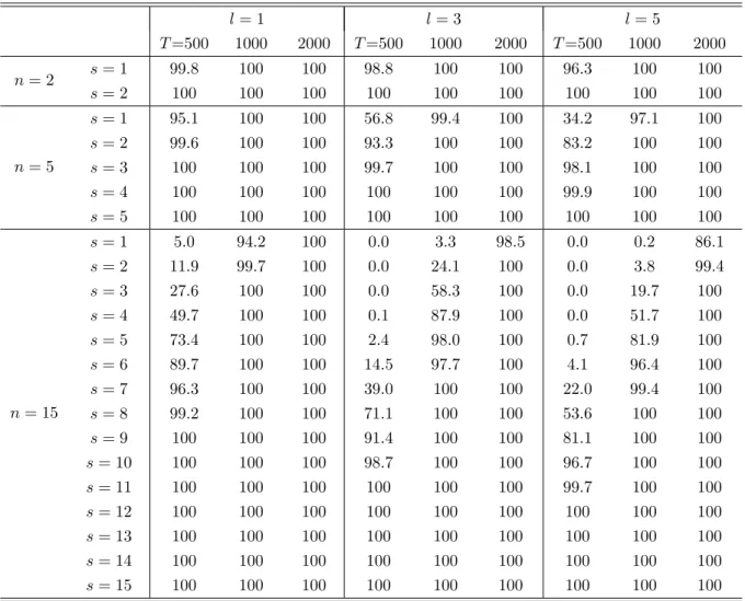
Let us then analyze the behavior of the pure variance estimated models on the log of the squared returns when the DGP is a diagonal VEC(0;1). Indeed we have seen that both the factor model and the diagonal model provide quite parsimonious marginal GARCH orders. We consequently investigate now whether some of the proposed strategies allow us to discriminate between these two models. We report in Table 2 the outcomes for di¤erent sample sizes forn= 2;5;15and l= 1;3;5in the estimated models. It emerges that except when T is small andl is large, the reduced rank procedure rejects quite well the presence of any common factors.
5
An illustrative example
The data set was obtained from TickData and consists of daily closing transaction prices for thirty large capi-talization stocks from the NYSE, AMEX NASDAQ, covering the period from January 1, 1999 to December 31, 2008 (2489 trading days). The appendix provides a list of ticker symbols and company names.
For the conditional mean we have estimated AR(2) models with daily dummies to capture Monday and Friday e¤ects. For the conditional variance we have run four di¤erent speci…cations. These are the GARCH(1,1), the GARCH(1,2) and two long memory models, namely FIGARCH(1; d;0) and FIGARCH(1; d;1). Out of the 30 series, the GARCH(1,1) model is favoured in six cases using both formal likelihood ratio tests and the Hannan-Quinn information criterion. The six returns with no indication of long memory are (and using their acronyms, see Appendix) ABT, BMY, GE, SLB, XOM, XRX.
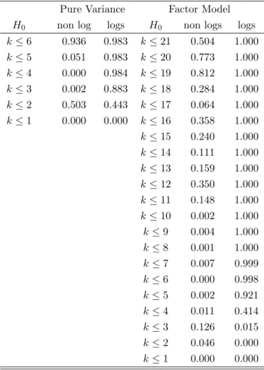
Therefore we consider these six return series and we apply our proposed test. The implications of FIGARCH type processes is out of the scope of this paper. Consequently the study of the other 24 series is left for further investigations. Table 3 shows the results for the pure variance model on the six squared returns only as well as the system that also includes their …fteen cross-products, hence with 21 series. We have considered for the moment2lags. The numbern korN kof linear combinations that do not have the GARCH feature gives the number kof factors generating the pure variance or the factor GARCH model. For the pure variance model in logs, a single common ARCH component generating the six returns is found, that is we takek= 1. The results would be di¤erent for the model in levels and/or when one also stacks the covariances. However, the simulation results of Section 4 revealed that the pure variance model for the logs of squared returns yields better results.
6
Conclusion and further research
This paper studies the orders of the marginal weak GARCH processes implied by a multivariate GARCH model. We see that except for some coincidental situation the marginal models are non-parsimonious. We then show
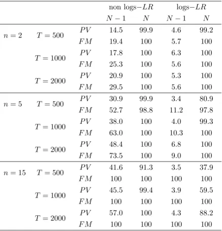
Table 1: Size and power of common volatility for the non-log version tests statistics non logs LR logs LR
N 1 N N 1 N n= 2 T = 500 P V F M 14:5 19:4 99:9 100 4:6 5:7 99:2 100 T = 1000 P V F M 17:8 25:3 100 100 6:3 5:6 100 100 T = 2000 P V F M 20:9 29:5 100 100 5:3 5:6 100 100 n= 5 T = 500 P V F M 30:9 52:7 99:9 98:8 3:4 11:2 80:9 97:8 T = 1000 P V F M 38:0 63:0 100 100 4:0 10:3 99:3 100 T = 2000 P V F M 48:4 73:5 100 100 6:8 9:0 100 100 n= 15 T = 500 P V F M 41:6 100 91:3 100 3:5 100 37:9 100 T = 1000 P V F M 45:5 100 99:4 100 3:9 100 59:5 100 T = 2000 P V F M 57:0 100 100 100 4:3 100 88:2 100
Note: The DGP has 1 source of volatility. Hence, the columnsN 1report the empirical size while the columnN
report the (size unadjusted) power. PV refers to the pure variance estimated model while FM refers to the factor model in which we also stack the covariances. l= 1in the estimated model. Non-logs LR columns refer to the likelihood ratio test on the vech or the diag of"t"0t;logs-LR columns refer to the likelihood ratio test on the vech or the diag of the matrix logs of"t"0t:Nominal size is 5%.
Table 2: Power of the PV common volatility for the log version tests statistics for the diagonal BEKK l= 1 l= 3 l= 5 T=500 1000 2000 T=500 1000 2000 T=500 1000 2000 n= 2 s= 1 s= 2 99:8 100 100 100 100 100 98:8 100 100 100 100 100 96:3 100 100 100 100 100 n= 5 s= 1 s= 2 s= 3 s= 4 s= 5 95:1 99:6 100 100 100 100 100 100 100 100 100 100 100 100 100 56:8 93:3 99:7 100 100 99:4 100 100 100 100 100 100 100 100 100 34:2 83:2 98:1 99:9 100 97:1 100 100 100 100 100 100 100 100 100 n= 15 s= 1 s= 2 s= 3 s= 4 s= 5 s= 6 s= 7 s= 8 s= 9 s= 10 s= 11 s= 12 s= 13 s= 14 s= 15 5:0 11:9 27:6 49:7 73:4 89:7 96:3 99:2 100 100 100 100 100 100 100 94:2 99:7 100 100 100 100 100 100 100 100 100 100 100 100 100 100 100 100 100 100 100 100 100 100 100 100 100 100 100 100 0:0 0:0 0:0 0:1 2:4 14:5 39:0 71:1 91:4 98:7 100 100 100 100 100 3:3 24:1 58:3 87:9 98:0 97:7 100 100 100 100 100 100 100 100 100 98:5 100 100 100 100 100 100 100 100 100 100 100 100 100 100 0:0 0:0 0:0 0:0 0:7 4:1 22:0 53:6 81:1 96:7 99:7 100 100 100 100 0:2 3:8 19:7 51:7 81:9 96:4 99:4 100 100 100 100 100 100 100 100 86:1 99:4 100 100 100 100 100 100 100 100 100 100 100 100 100
Note: The DGP hasnsource of volatility withinnvariables. This is the diagonal VEC(0,1). We report the power of the pure variance estimated model with the log version.
Table 3: P-Value of LR tests (2 lags) for both the pure variance and the factor model Pure Variance Factor Model
H0 non log logs H0 non logs logs
k 6 0.936 0.983 k 21 0.504 1.000 k 5 0.051 0.983 k 20 0.773 1.000 k 4 0.000 0.984 k 19 0.812 1.000 k 3 0.002 0.883 k 18 0.284 1.000 k 2 0.503 0.443 k 17 0.064 1.000 k 1 0.000 0.000 k 16 0.358 1.000 k 15 0.240 1.000 k 14 0.111 1.000 k 13 0.159 1.000 k 12 0.350 1.000 k 11 0.148 1.000 k 10 0.002 1.000 k 9 0.004 1.000 k 8 0.001 1.000 k 7 0.007 0.999 k 6 0.000 0.998 k 5 0.002 0.921 k 4 0.011 0.414 k 3 0.126 0.015 k 2 0.046 0.000 k 1 0.000 0.000
that multivariate models with co-movements in the conditional volatility and cross products explain why we can obtain GARCH with small orders in empirical work. This result would plead for looking at individual series prior to a multivariate modelling.
We propose a simple strategy to detect the presence of such GARCH co-movements and we apply it to daily returns from the NASDAQ. It emerges that when working with the six returns (out of 30) having parsimonious univariate GARCH speci…cations we detect the presence of a single factor generating the volatility.
From our Monte Carlo study, the best strategy consists in applying the method proposed by Engle and Marcucci (2006) for the logs of the squared returns (i.e. the pure variance model), omitting therefore the cross-products (although they might matter in theory).
Many issues are currently under investigation. First we have focussed on a limited number of multivariate models. We have not covered stochastic volatility models, or alternative multivariate models (GO-GARCH, DECO,...). Second, we have still to study the properties of the tests proposed using appropriate estimators of the asymptotic standard-errors of the QMLE and investigate the behavior of bootstrap procedures to estimate standard-errors and to test for the number of common factors in multivariate weak GARCH processes.
Third, our test statistics seems to be tailored for multivariate GARCH(0; q) but we have not extensively investigated in our Monte Carlo study its use in more general multivariate GARCH(p; q) although results for the marginalization orders of the multivariate GARCH(p; q) are given in this paper. Whether this multivariate modelling is more appropriate than a GARCH(0,q) is an empirical issue. In order to work in this framework, and for separating the MA from the AR part possibly with matrices with di¤erent left null spaces, we believe that another testing strategy should be implemented. A promising procedure we leave for further investigations relies on realized variance and covariances.
7
References
Baba, Y., R.F. Engle, D.F. Kraft, and K.F. Kroner (1989), Multivariate Simultaneous Generalized ARCH, DP 89-57 San Diego.
Bauwens, L., S. Laurent and J.V.K. Rombouts (2006), Multivariate GARCH Models: a Survey,
Journal of Applied Econometrics 21, 79–109.
Billio M., M. Caporin and M. Gobbo (2003), Block Dynamic Conditional Correlation Multivariate GARCH Models, Working paper 0303 GRETA, Venice.
Comte, F. and O. Lieberman (2003), Asymptotic Theory for Multivariate GARCH Processes,Journal of Multivariate Analysis 84, 61-84.
Cubadda, G., Hecq A. and F.C. Palm .(2008),Macro-panels and Reality, Economics Letters, 99, 537-540.
Cubadda, G., Hecq A. and F.C. Palm (2009), Studying Interactions without Multivariate Modeling, Journal of Econometrics,148, 25-35.
forthcoming inJournal of Forecasting.
Drost, F.C. and T.E. Nijman (1993), Temporal Aggregation of GARCH Processes, Econometrica 61, 909-927.
Engle, R. F., V. Ng and M. Rothschild (1990), Asset Pricing With a Factor ARCH Covariance
Structure: Empirical Estimates of Treasury Bills,Journal of Econometrics, 45, 213-238.
Engle, R. F. and B. Kelly (2008),Dynamic Equicorrelation, Stern School of Business, WP NYU.
Engle, R. F. and S. Kozicki (1993),Testing for Common Features (with Comments),Journal of Business and Economic Statistics, 11, 369-395.
Engle, R. F. and J. Marcucci (2006), A Long-run Pure Variance Common Features Model for the
Common Volatilities of the Dow Jones,Journal of Econometrics, 132, 7-42.
Francq, C. and J.-M. Zakoian (2007), HAC Estimation and Strong Linearity Testing in Weak ARMA Models,Journal of Multivariate Analysis 98, 114-144.
Jeantheau, T. (1998), Strong Consistency of Estimators for Multivariate ARCH Models, Econometric Theory 15, 70-86.
Nijman, T. and E. Sentana (1996), Marginalization and Contemporaneous Aggregation in Multivariate GARCH Processes,Journal of Econometrics, 71, 71-87.
Silvennoinen, A. and T. Terasvirta (2009),Multivariate GARCH Models, Handbook of Financial Time Series, Ed. Andersen, T.G. and Davis, R.A. and Kreiss, J.P. and T. Mikosch, Sringer.
Tiao, G. C. and R. S. Tsay (1989), Model Speci…cation in Multivariate Time Series (with Comments), Journal of Royal Statistical Society, Series B, 51, 157-213.
Zellner, A. and F.C. Palm (1974),Time Series Analysis and Simultaneous Equation Econometric Models, Journal of Econometrics 2, 17-54.
Zellner, A. and F.C. Palm (1975), Time Series and Structural Analysis of Monetary Models of the US Economy,Sanhya: The Indian Journal of Statistics, Series C 37, 12-56.
Zellner, A. and F.C. Palm (2004), The Structural Econometric Time Series Analysis Approach, Cam-bridge University Press.
8
Stocks used in the empirical application
Symbol Issue name Symbol Issue nameAAPL APPLE INC JNJ JOHNSON &JOHNSON
ABT ABBOTT LABORATORIES JPM JP MORGAN CHASE AXP AMERICAN EXPRESS CO KO COCA COLA CO
BA BOEING CO LLY ELI LILLY & CO
BAC BANK OF AMERICA MCD MCDONALDS CORP
BMY BRISTOL MYERS SQ MMM 3M COMPANY
BP BP plc MOT MOTOROLA
C CITIGROUP MRK MERCK & CO
CAT CATERPILLAR MS MORGAN STANLEY
CL COLGATE-PALMOLIVE CO MSFT MICROSOFT CP
CSCO CISCO SYSTEMS ORCL ORACLE CORP
CVX CHEVRON CORP PEP PEPSICO INC
DELL DELL INC PFE PFIZER INC
DIS WALT DISNEY CO PG PROCTER & GAMBLE
EK EASTMAN KODAK QCOM QUALCOMM
EXC EXELON CORP SLB SCHLUMBERGER N.V.
F FORD MOTOR CO T AT&T CORP
FDX FEDEX CORP TWX TIME WARNER
GE GENERAL ELEC UN UNILEVER N V
GM GENERAL MOTORS VZ VERIZON COMMS
HD HOME DEPOT INC WFC WELLS FARGO & CO
HNZ H J HEINZ CO WMT WAL-MART STORES
HON HONEYWELL INTL WYE WEYERHAEUSER CO
IBM INTL BUS MACHINE XOM EXXON MOBIL