LEVERAGING METALEARNING FOR BAGGING
CLASSIFIERS
FÁBIO HERNÂNI DOS SANTOS COSTA PINTO
TESE DE DOUTORAMENTO APRESENTADAÀ FACULDADE DE ENGENHARIA DA UNIVERSIDADE DO PORTO EM ENGENHARIA INFORMÁTICA
F´
abio Hernˆ
ani dos Santos Costa Pinto
Leveraging Metalearning for Bagging
Classifiers
Tese apresentada `a Faculdade de Engenharia da Universidade do Porto para obten¸c˜ao do grau de Doutor em Engenharia Inform´atica,
realizada sob orienta¸c˜ao cient´ıfica do
Prof. Doutor Carlos Manuel Milheiro de Oliveira Pinto Soares, Professor Associado da Faculdade de Engenharia da Universidade do Porto,
e co-orienta¸c˜ao cient´ıfica do
Prof. Doutor Jo˜ao Pedro Carvalho Leal Mendes Moreira,
Professor Auxiliar da Faculdade de Engenharia da Universidade do Porto
Departamento de Engenharia Inform´atica Faculdade de Engenharia da Universidade do Porto
Aos meus pais, porque eu escrevi a tese mas eles fizeram tudo o resto.
Abstract
Machine Learning (ML) has been successfully applied to a wide range of domains and applications. One of the techniques behind most of these successful appli-cations is Ensemble Learning (EL), the field of ML that gave birth to supervised learning methods such as bagging, Random Forests or boosting.
The level of expertise required to successfully apply ML techniques to busi-ness problems is often very high. This, together with the market scarcity on ML experts, has increased the need for systems that can accelerate and improve the learning process. In this thesis, we focus on how to use metalearning (MtL), the field of ML that studies how learning can be used to solve learning problems, to automate and improve the performance of bagging, one of the most popular EL algorithms.
The scientific contributions of this thesis are split into two parts of this vol-ume: Automated Machine Learning (autoML) in part II and Ensemble Learning
in part III. In part II, we extend the state-of-the-art in metalearning andautoML
with the following contributions: 1) a MtL framework for systematic generation
of metafeatures and 2) anautoML system that combines MtL with a learning
to rank approach to automatically generate a bagging ensemble.
In part III, we make the following contributions: 1) a method that uses MtL to prune bagging ensembles by analysing the data characteristics of the bootstrap samples that are generated and 2) a MtL method to dynamically combine a subset of predictors from an ensemble according to the characteristics of a given test instance.
In both parts, our contributions show that MtL can be an important com-ponent of the learning systems of the future. Some of the methods have been published in research papers and therefore, this thesis also serves as a
Resumo
A ´area de Machine Learning (ML) tem sido aplicada com sucesso numa
am-pla gama de dom´ınios e aplica¸c˜oes. Um dos conjuntos de t´ecnicas mais
bem-sucedidas ´eEnsemble Learning (EL), a ´area de ML que deu origem a m´etodos
de aprendizagem supervisionada comobagging,Random Forests ouboosting.
O n´ıvel de expertise necess´ario para aplicar t´ecnicas de ML a problemas
industriais ´e tipicamente bastante alto. Este facto, juntamente com a escassez no mercado em especialistas em ML, criou a necessidade de sistemas que possam acelerar e melhorar o processo de aprendizagem. Nesta tese,
concentramos-nos em como podemos usar metalearning (MtL), a ´area de ML que estuda
como a aprendizagem pode ajudar a resolver problemas de aprendizagem, para
automatizar ou melhorar o desempenho debagging, um dos algoritmos de EL
mais utilizados na ind´ustria.
As contribui¸c˜oes cient´ıficas desta tese est˜ao divididas em duas partes deste
volume: Automated Machine Learning(autoML) na parte II eEnsemble
Learn-ing na parte III. Na parte II, estendemos o estado da arte em autoMLcom as
seguintes contribui¸c˜oes: 1) umframework de MtL para gera¸c˜ao sistem´atica de
metafeatures e 2) um sistemaautoML que combina MtL com uma t´ecnica de
ranking para afina¸c˜ao autom´atica dos componentes de um modelo bagging. Na parte III, fazemos as seguintes contribui¸c˜oes: 1) um m´etodo que usa MtL
para fazer pruning de modelos bagging, atrav´es da an´alise das caracter´ısticas
da amostras bootstrap que s˜ao geradas e 2) um m´etodo MtL para combinar
dinamicamente um subconjunto de modelos de umensemble de acordo para as
caracter´ısticas de cada instˆancia de teste.
Em ambas as partes, as nossas contribui¸c˜oes mostram que MtL pode ser uma
componente importante dos sistemas de aprendizagem do futuro. Alguns dos vii
m´etodos foram publicados como artigo cient´ıficos e, portanto, esta tese tamb´em
Agradecimentos
Hoje ´e dia 18 de Janeiro de 2018 e estou sentado no sof´a c´a de casa a terminar
a escrita desta tese que comecei por volta de Outubro de 2013. Foram 4 anos
e alguns meses de muito trabalho. Estes agradecimentos v˜ao ser o ´ultimo texto
que acrescento. Enquanto oi¸co Bowie. A seguir vem The Doors e Nick Drake, segundo a playlist. N˜ao vou come¸car j´a a agradecer. Vou come¸car por expressar o qu˜ao farto estou de trabalhar nisto! Tem de ser. Estou t˜ao cansado de corrigir
typos que vou deixar aqui um de prop´ositto. Odeio tanto a tese neste momento como adorei fazˆe-la nestes anos. Yup. Valeu a pena. Aprendi muito mesmo.
Tenho de come¸car pelo Carlos. Porque de facto come¸cou com ele a convencer-me que conseguia fazer um doutoraconvencer-mento. Eu? Doutoraconvencer-mento? Nunca convencer-me tinha passado pela cabe¸ca! No entanto, tive a sorte de ter um orientador de mestrado e doutoramento que ´e um daqueles raros professores que conseguem transformar um aluno mediano e desmotivado em algu´em que acredita que pode chegar ao grupo dos melhores. Talvez pela confian¸ca que passa... sinceramente ainda n˜ao percebi muito bem qual ´e o truque. Lembro-me de pensar ”se este gajo acha que posso ser um dos melhores, ent˜ao ´e porque posso mesmo!”. E isso faz toda a diferen¸ca. Mesmo! Ensinas a quem est´a disposto a aprender e acreditas cegamente no aluno. N˜ao podia pedir mais. Aprendi muito contigo. N˜ao sei se tens no¸c˜ao do enorme impacto que tiveste na minha vida e provavelmente nunca vou conseguir expressar-me de forma a que isso fique claro. Obrigado! Como ´es tamb´em um amigo e um bacano, vamos continuar a ver-nos por a´ı, nem que seja
naqueles concertos manhosos de indie do Primavera que s´o tu gostas. E este
pensamento fez-me lembrar que no meio de todas as virtudes tens um enorme
defeito: como ´e poss´ıvel n˜ao gostar de Pink Floyd?!?
Professor Jo˜ao. Outro bacano! E que tamb´em est´a sempre l´a, mesmo quando
parece nem ter tempo para respirar. Ajudou-me imenso a pensar e formalizar
problemas com rigor cient´ıfico. Sabe tudo o que h´a para saber sobre
Ensem-ble Learning, parece que tem uma biblioteca na cabe¸ca. E sempre com uma
humildade incr´ıvel. N˜ao podia pedir melhor co-orientador tamb´em
H´a mais duas pessoas que tiveram um impacto direto neste trabalho `as
quais n˜ao posso deixar de agradecer: o V´ıtor e o Professor Pavel. Ao Bit´o por
ser aquele gajo t´ımido que parece que se esfor¸ca por passar despercebido mas inevitavelmente vai-se tornar num dos melhores investigadores portugueses em Machine Learning. Para mim foi super importante come¸car a colaborar contigo nesta fase final da tese, deu-me aquela pica que faltava para conseguir acabar isto bem e como eu queria. Depois do MLj vamos ao JMLR, andamento nisso!
Ao Professor Pavel por ser um vision´ario, mentor e extraordin´ario investigador.
N˜ao me lembro de ter uma conversa consigo em que n˜ao tivesse aprendido alguma coisa. Recordo-me agora daquele jantar do ECML de 2016 em que lhe perguntei quando foi a primeira vez que ouviu falar no termo metalearning... ”o termo metalearning? Fui eu que inventei! Pois, est´a claro!” Pfff, estudasses! Clar´ıssimo!
Acho que a tese tamb´em se fez pelo contexto em que estava inserido e mais uma vez n˜ao podia pedir mais. O LIAAD 1.0 que me recebeu em 2013 h´a-de ser sempre um dos melhores grupos de investiga¸c˜ao que um aluno de doutoramento pode desejar. Do dia para a noite vi-me rodeado de alguns dos melhores jovens investigadores de Machine Learning da minha gera¸c˜ao: (liaad = c(”Cl´audio”, ”M´arcia”, ”Pedro”); sample(liaad)), Matias, Rafa, Rui, Vˆania, Douglas, Jo˜ao, Concei¸c˜ao e S´oninha. Ao LIAAD 2.0/CESE, que fizeram renascer os almo¸cos: Tiago, Jo˜ao, Catarina, Dario, Bruno, Joana, Maria Jo˜ao, Miguel, Kemily. Aos
malucos que passaram pelo INESC. `A minha equipa na Farfetch, que me ajudou
a ser um melhor cientista dos dados: Jo˜ao, Lage, Ana, Paula, Carvalheira,
Andreia, Antonieta, Otto; `a malta que queria ser de recomenda¸c˜oes mas n˜ao ´e: Ana, Lia, Ricardo, Ba´ıa e Hugo. E ao Carlos e Cristina pela incr´ıvel aposta que fizeram em mim!
Aos meus amigos, eles sabem quem s˜ao. Aos amigos do rock, por me
aju-darem a descarregar energia `as quarta-feiras a fazer algo que tanto gosto: Jos´e
xi `
A m´usica. `As minhas guitarras. Aos livros. `A Nova Zelˆandia. `A Becky e ao
Kiko. Aos que c´a n˜ao est˜ao mas deviam estar. `A piripupi. Aos que ir˜ao estar.
Acknowledgements
This PhD thesis is partially funded by FCT/MEC through PIDDAC and ERD-F/ON2 within project NORTE-07-0124-FEDER-000059, a project financed by the North Portugal Regional Operational Programme (ON.2 O Novo Norte), under the National Strategic Reference Framework (NSRF), through the Eu-ropean Regional Development Fund (ERDF); partially funded by the ECSEL Joint Undertaking, the framework programme for research and innovation hori-zon 2020 (2014-2020) under grant agreement number 662189-MANTIS-2014-1; and by national funds, through the Portuguese funding agency, Funda¸c˜ao para a Ciˆencia e a Tecnologia (FCT), within project UID/EEA/50014/2013.
Contents
I
Prologue
1
1 Introduction 3
1.1 Problem Overview . . . 4
1.2 Research Question and Contributions . . . 5
1.2.1 Contributions . . . 6
1.3 Structure of this thesis . . . 6
2 Overview 9 2.1 Error, Accuracy and Diversity in Ensembles . . . 9
2.2 Bagging, Boosting and other EL algorithms . . . 12
2.3 Ensemble Generation . . . 14 2.3.1 Data manipulation . . . 14 2.3.2 Model generation . . . 15 2.4 Ensemble Pruning . . . 16 2.4.1 Partitioning-based . . . 16 2.4.2 Search-based . . . 16 2.5 Ensemble Integration . . . 17 2.5.1 Static . . . 18 2.5.2 Dynamic selection . . . 19 2.5.3 Dynamic combination . . . 20 2.6 Metalearning . . . 22 2.6.1 Metadata . . . 23 2.6.2 Applications . . . 26 xv
II
Automated Machine Learning
33
3 Systematic Generation of Metafeatures 35
3.1 Introduction . . . 35
3.2 Metalearning . . . 37
3.2.1 Types of metafeatures . . . 37
3.2.2 Domains of application . . . 38
3.2.3 Methodologies for metafeature design . . . 40
3.3 Systematic Generation Of Metafeatures . . . 41
3.3.1 Basic Concepts . . . 42
3.3.2 Algorithm . . . 44
3.3.3 Example . . . 45
3.4 Fitting Common Metafeatures in the Framework . . . 46
3.5 Experiments . . . 50
3.5.1 Base-level experimental setup . . . 51
3.5.2 Meta-level experimental setup . . . 51
3.5.3 Systematic sets of metafeatures . . . 52
3.5.4 Systematic vs non-systematic . . . 53
3.5.5 Systematic vs state-of-the-art . . . 56
3.5.6 Generating novel sets of systematic metafeatures . . . 58
3.6 Discussion . . . 60
3.7 Conclusions and Future Work . . . 62
4 autoBagging: Automated Bagging Ensembles 65 4.1 Introduction . . . 65
4.2 Related Work . . . 67
4.2.1 Metalearning based . . . 68
4.2.2 Optimization based . . . 68
4.2.3 Optimization and metalearning . . . 69
4.2.4 Ensemble focused autoML . . . 69
4.3 Bagging Workflows . . . 70
4.3.1 Generation . . . 71
4.3.2 Pruning . . . 71
CONTENTS xvii
4.4 autoBagging: Ranking Bagging Workflows . . . 72
4.4.1 Learning Approach . . . 73
4.4.2 Metafeatures . . . 73
4.4.3 Metatarget . . . 75
4.5 Experiments . . . 75
4.5.1 Experimental setup . . . 76
4.5.2 Exploratory metadata analysis . . . 78
4.5.3 Results . . . 79
4.6 Conclusions and Future Work . . . 85
III
Metalearning for Ensemble Learning
87
5 Analysing and Pruning Bagging 89 5.1 Introduction . . . 895.2 Related Work . . . 91
5.2.1 Understanding bagging . . . 92
5.2.2 Pruning bagging ensembles . . . 93
5.3 Empirical Methodology to Characterize Bagging Performance . . 94
5.3.1 Estimating the distribution of performance by sampling . 94 5.3.2 Discussion . . . 96
5.4 Generating Metadata . . . 97
5.5 What Makes a Good Bootstrap? . . . 99
5.5.1 Exploratory analysis . . . 100
5.6 Pruning Bagging Ensembles with Metalearning . . . 104
5.6.1 Experimental setup . . . 106
5.6.2 Results . . . 107
5.6.3 Discussion . . . 110
5.7 Conclusions and Future Work . . . 110
6 CHADE: CHAined Dynamic Ensemble 113 6.1 Introduction . . . 113
6.2 Related Work . . . 115
6.2.1 Dynamic selection . . . 115
6.3 CHADE . . . 117
6.4 Experiments . . . 120
6.4.1 Experimental setup . . . 121
6.4.2 Comparison with another MtL approach . . . 122
6.4.3 Comparison with state-of-the-art . . . 124
6.5 Further Analysis . . . 126
6.6 Conclusions and Future Work . . . 129
IV
Epilogue
131
7 Conclusions 133 7.1 Future Research . . . 137List of Figures
2.1 Metalearning framework for algorithm recommendation. . . 23
2.2 Metafeatures taxonomy. Source: Brazdilet al. [2009]. . . 24
3.1 Metalearning framework for algorithm recommendation. . . 38
3.2 Framework for the systematic development of metafeatures. . . . 42
3.3 This schema illustrates the application of the framework in the
example learning scenario provided in the text. . . 46
3.4 Metafeatures represented using our framework. . . 47
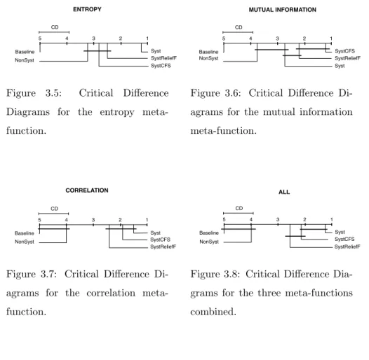
3.5 Critical Difference Diagrams for the entropy meta-function. . . . 55
3.6 Critical Difference Diagrams for the mutual information
meta-function. . . 55
3.7 Critical Difference Diagrams for the correlation meta-function. . 55
3.8 Critical Difference Diagrams for the three meta-functions combined. 55
3.9 Critical Difference diagrams of systematic metafeatures Vs
state-of-the-art. . . 57
3.10 Critical Difference diagrams comparing the set of metafeatures generated by Pearson’s correlation with the set generated by MIC. 59 3.11 Critical Difference diagrams comparing the set of mefeatures
gen-erated by mutual information with the set gengen-erated by
interac-tion informainterac-tion. . . 60
4.1 Learning to Rank with MtL. The red lines represent offline tasks
and the green ones represent online ones. . . 67
4.2 Boxlplots of the kappa values collected for each dataset from
eval-uating the performance of each bagging workflow. . . 79
4.3 Boxplots of the ranking scores collected for each bagging
work-flow. For instance,200bb0.75knora-e represents a bagging
work-flow with 200 trees, to which boosting-based pruning is applied with a 75% cut point and KNORA-E is used as dynamic
integra-tion technique. . . 80
4.4 Critical Difference diagram (withα= 0.05) of the experiments. . 80
4.5 Violin and boxplots showing the distribution of execution time for
the methodautoBagging@1, autoBagging@3,autoBagging@5and
averageRank@1 in comparison withauto-sklearn. We computed the ratio of the execution time of each method in seconds by the execution time of auto-sklearn (3600 seconds). The logarithmic transformation was applied for visualization purposes. The red
line represents the execution time ofauto-sklearn, since log(1) = 0. 82
4.6 Loss curve comparing autoBagging with the Average Rank method. 83
4.7 Critical difference diagram comparing autoBagging with the
Av-erage Rank method. . . 83
4.8 Top 30 most important metafeatures for theXGboost metamodel
measured usingGain, which represents the relative contribution
of the corresponding feature to the model calculated by taking
each feature’s contribution for each tree in the model. . . 84
5.1 KLD between % of sample and population. Each line represents
a different dataset. . . 95
5.2 Mean KLD (and standard deviation) between % of sample and
population. . . 95
5.3 Sampling and Kullback-Leibler Divergence, averaged for all datasets. 96
5.4 Density plot for a 10 % sample and population of thedis dataset.
The KLD between this sample and population is 30.89. . . 97
5.5 Density plot for a 10 % sample and population of theacetylation
dataset. The KLD between this sample and population is 0.23. . 97
5.6 Boxplot of numeric metatarget (k=100) vs classes found by
Fisher-Jenks algorithm. . . 101
5.7 Boxplot of numeric metatarget (k=20) vs classes found by
LIST OF FIGURES xxi
5.8 Pairwise Wilcoxon Rank Sum test for multiple comparison
pro-cedures (k=20). Black dot represents a significative difference
between the pair of classes. . . 102
5.9 Pairwise Wilcoxon Rank Sum test for multiple comparison
pro-cedures (k=100). Black dot represents a significative difference
between the pair of classes. . . 102 5.10 Boxplot and density distribution of the Jensen-Shannon distance
withk=100. . . 102
5.11 Boxplot and density distribution of the Jensen-Shannon distance
withk=20. . . 102
5.12 Density distribution of the metafeatures Q-Statistic and COD for
thek=100 experiment. . . 103
5.13 Density distribution of the metafeatures Q-Statistic and COD for
thek=20 experiment. . . 103
5.14 Density distribution of the landmakers Decision Stump and Naive
Bayes for thek=100 experiment. . . 104
5.15 Density distribution of the landmakers Decision Stump and Naive
Bayes for thek=20 experiment. . . 104
5.16 Schema of the approach for pruning bagging ensembles with MtL. 105 5.17 Critical Difference diagrams of the performance of the
meta-models in comparison with the baseline, at the meta-level. . . 108 5.18 Critical Difference diagrams of the performance of the
metamod-els in comparison with the benchmark pruning methods, at the base-level. . . 109
6.1 CHADE framework. . . 118
6.2 Critical Difference diagrams (withα= 0.05) for the comparison
with META-DES at the meta-level. The null hypothesis of the
Friedman’s test is rejected forα= 0.01, 0.05 and 0.1. . . 123
6.3 Critical Difference diagrams (withα= 0.05) for the comparison
with META-DES at the base-level. The null hypothesis of the
6.4 Critical Difference diagrams (with α = 0.05) for the compari-son with several dynamic selection/combination methods at
base-level. The null hypothesis of the Friedman’s test is rejected forα
= 0.01, 0.05 and 0.1. . . 125
6.5 Evolution of the base-level mean rank as more meta-models are
added to E-CHADE. . . 125
6.6 Evolution of the meta-level mean rank as more meta-models are
added to E-CHADE. . . 125
6.7 XOR problem. . . 127
6.8 Heat maps showing the combination of classifiers made by each
technique. . . 127
6.9 Distribution of the number of classifiers selected per instance by
each method. . . 128 6.10 Distribution of the number of times each classifier was selected
List of Tables
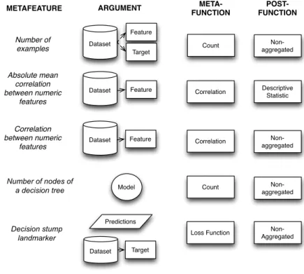
3.1 Some examples of metafeatures that have been used for MtL. . . 41
3.2 Results comparing the systematic metafeatures generated with
meta-functions entropy, mutual information and correlation in
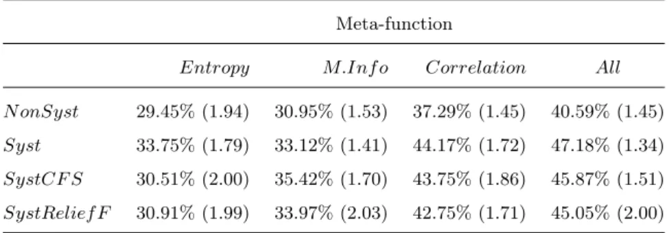
comparison with the non-systematic.SystCF SandSystRelief F
represent the systematic sets after feature selection with the meth-ods CFS and ReliefF, respectively. The baseline achieves an aver-age 22.65% accuracy on all experiments. The standard deviation
of the values is between parentheses. . . 54
3.3 Systematic sets of metafeatures in comparison with
state-of-the-art metafeatures. The baseline achieves a 22.65% accuracy on all experiments. The standard deviation of the values is between
parentheses. . . 57
3.4 Comparison of the sets of metafeatures generated by Pearson’s
correlation and MIC. The baseline achieves a 40% accuracy on all experiments. The standard deviation of the values is between
parentheses. . . 59
3.5 Comparison of the sets of metafeatures generated by mutual
in-formation and interaction inin-formation.The baseline achieves a 22.65% accuracy on all experiments. The standard deviation of
the values is between parentheses. . . 60
3.6 List of the top 3 metafeatures in terms of variable importance for Random Forests meta-models. For each set of features, we gener-ated a meta-model using Random Forests as meta-learner using all the metadata collected from the 206 datasets. The variable
importance is measured using the mean decrease in Gini index. . 61
5.1 Relationship between a pair of classifiers in a bootstrapb and a
datasetd. . . 98
6.1 Example of a meta-training datasetD’. . . 119
Part I
Prologue
Chapter 1
Introduction
The fusion and exponential growth of technologies is giving rise to what some call a Fourth Industrial Revolution [Schwab, 2017]. This process is creating an overlap between the boundaries of the physical and digital world. At the core of this technological turmoil, we find artificial intelligence, machine learning, and more specifically, the ability to learn from data. And today’s world is deluged by data.
The dissemination of the Internet around the globe together with the devel-opment of ubiquitous information-sensing mobile devices, wireless sensor net-works and information store capacity, has enhanced the need to understand and make value of the data that is being generated. Data Science, a recently coined term that brings together statistics, machine learning and computer science, emerges as the field that can assist humans in this task [Miller, 2013]. Research on machine learning plays a central role in the development of this field since it provides the techniques and methods that enable to learn from data.
One of the most common challenges raised by this huge volume of data is focused on supervised learning: the task of generating a function that represents the relationship between a set of variables and a label (classification) or numeric variable (regression). This kind of problem can be seen in multiple applications
(finance, retail, banking, industry, to name a few - Hanet al.[2006]). Several
techniques have been proposed for supervised learning. From a predictive per-formance perspective, ensemble learning (EL) methods are one of the groups
of techniques that present better performance [Zhou, 2012]. EL is a process that uses a set of models (regression or classification), each of them obtained by applying a learning process to a given problem. This set of models is integrated
in some way to obtain the final prediction [Mendes-Moreiraet al., 2012]. EL has
become increasingly popular both for regression and classification tasks. Besides the extensive research that reports great results with ensemble algorithms in a wide variety of problems [Zhou, 2012], data mining competitions with great me-dia coverage (for instance, Netflix prize, Heritage Health prize, among others) proved that ensembles are among the top techniques for predictive modelling.
1.1
Problem Overview
In the past few years, the growth of data volume, velocity and variety has increased dramatically the demand for data scientists, particularly in the in-dustry [Columbus, 2017]. This shortage of data science experts is particularly notorious in specific skills, such as deep learning or EL, since these are the techniques that dominate the state-of-the-art in several domains. Moreover,
the lack of data scientists together with the data explosion (which per se
cre-ates more opportunities for machine learning applications), crecre-ates the need for tools that can enhance data scientists’ productivity. The resulting research field
that aims to answers these needs is automated machine learning (autoML), by
merging ideas and techniques from several ML and optimization topics, such as Bayesian optimization, metalearning and combinatorial optimization. We will
focus particularly onmetalearning.
Metalearning (MtL), as defined by Brazdil et al. [2009], is “the study of
principled methods that exploit metaknowledge to obtain efficient models and solutions by adapting machine learning and data mining processes”. In this thesis, we study how MtL can be used as a mechanism to automate or improve machine learning processes, specifically, EL methods.
Mendes-Moreira et al. [2012] split EL research into three topics: ensemble
generation (how to generate the single models that constitute the ensemble), pruning (how to prune an ensemble after its generation to reduce its size and eventually improve performance) and integration (how to combine the single
1.2. RESEARCH QUESTION AND CONTRIBUTIONS 5 models that constitute the ensemble to make a final prediction). We adapt the same structure of the literature and we focus on specific problems in each topic:
Ensemble generation. When combining several models for a predictive task, it is difficult to understand the behaviour of the resulting ensemble and why it performs well or not. The models of an ensemble need to be complementary in different regions of the input space but measuring diversity is a very difficult task [Kuncheva and Whitaker, 2003]. Therefore, this has led diversity to become a topic of paramount importance for the EL field, both from a theoretical and
a practical perspective [Brownet al., 2005].
Ensemble pruning. Research on EL has shown that it is possible to reduce the size of an ensemble without loss of performance. In some cases, researchers
even reported predictive gains [Zhou et al., 2002]. These findings led to the
development of several methods for ensemble pruning [Martinez-Mu˜noz et al.,
2009], particularly useful for the scenarios in which the computational resources
are scarce [Qianet al., 2015].
Ensemble integration. Using an ensemble to obtain predictions is usu-ally a straightforward process. If we generate an ensemble that our evaluation methodology estimates to be accurate, that model is going to be used to score any instance that we want to predict, regardless of its characteristics. An al-ternative to this is a dynamic approach: automatically select one or more pre-dictive models from an ensemble according to the characteristics of a given test instance.
From a practical point-of-view, designing an ensemble that takes into account all this stages can be very complex, particularly for a data scientist that is a non-expert in EL. Furthermore, we believe that each one of this stages of EL can be improved by learning from past experience, which often is discarded by EL algorithms.
1.2
Research Question and Contributions
One of the earliest and most influential EL algorithms is bagging [Breiman, 1996a] (pseudo code is provided in section 2.2). Since its also one of the most widely used EL algorithms both in the academic world as in the industry (and
one of the building foundations of Random Forests, which is one of the most popular algorithms these days), we selected it as our object of study. Therefore, in this PhD thesis, we want to test the validity of the following hypothesis:
Is it possible to automate and improve the performance of bagging by using metalearning?
Naturally, the scope of this hypothesis is wide enough to associate it with a possibly infinite number of sub-problems. We do not aim to solve them all. Our main focus is to understand the state-of-the-art in bagging and bagging-related methods focusing on ensemble generation, pruning and integration; identify gaps that can be fulfilled by MtL systems; and finally design, evaluate and propose those systems.
1.2.1
Contributions
The contributions of this thesis are briefly summarised as follows:
• A MtL framework for systematic generation of metafeatures.
• New metafeatures that we show to be informative for characterizing datasets,
particularly for the algorithm selection problem.
• AnautoMLsystem that combines MtL with a learning to rank approach to automatically optimize a bagging ensemble.
• An empirical methodology to study the behaviour of bagging and give
insights about the desired properties of a bagging ensemble.
• A method that uses MtL to prune bagging ensembles by analysing the
data characteristics of the bootstrap samples that are generated.
• A MtL method to dynamically combine a subset of predictors from an
ensemble according to the characteristics of a given test instance.
1.3
Structure of this thesis
1.3. STRUCTURE OF THIS THESIS 7
• Part I: Prologue. This part combines chapters 1 and 2 of this thesis, serving as introduction and overview of the topics explored, respectively. Chapter 2 provides a brief overview of the state-of-the-art both for EL and MtL, focusing particularly on the intersection between the two. However, it is important to notice that, for each chapter of this thesis, we provide a specific section in which we detail the related work of each contribution in the chapter.
• Part II: Automated Ensemble Learning. This part includes
chap-ters 3 and 4. In the former, we propose aMtL framework that enables the
generation of metafeatures in a systematic fashion. Although we present and evaluate the framework for algorithm selection in classification prob-lems, the framework can be generalized for other ML problems. In fact, this is accomplished in chapter 4, in which we use the framework together
with a learning to rank approach to design anautoML system that is able
to automatically rank bagging workflows.
• Part III: Metalearning for Ensemble Learning. In this part we com-prise the chapters that provide contributions for the three sub-fields of EL: generation, pruning and integration. In chapter 5, we propose an empiri-cal methodology for the analysis of the behaviour of the bagging algorithm using MtL. In the same chapter, we use the metadata collected from
ap-plying the methodology to introduce an ensemble pruning technique for
bagging ensembles. Finally, in chapter 6, we design and propose a MtL system for dynamic integration of ensembles for classification problems.
• Part IV: Epilogue. The final part of the thesis is composed by chapter 7, that concludes the volume summarizing the work done and addressing the research question defined initially. Finally, ideas for future research are suggested.
Chapter 2
Overview
In this section, we describe an overview of the literature for the two main sub-fields of ML that we address in this thesis: EL and MtL. We focus particularly on papers that somehow relate these two sub-fields.
2.1
Error, Accuracy and Diversity in Ensembles
Historically, the two pioneering papers that laid the roots for EL research pre-sented different perspectives on the same subject: Hansen and Salamon [1990] published an empirical work in which was found that predictions made by an ensemble of classifiers (neural networks) are often more accurate than the best single classifier. On the other hand, Schapire [1990] showed theoretically that weak learners can be combined to form a strong learner which settled the basic concept behind Boosting algorithms.
EL literature is very clear about what characteristics a good ensemble must
present: the predictors must beaccurate and diverse in order to complement
themselves. The concept of complementarity is very important. Combining complementary classifiers can improve the accuracy over individual models. One can say that two classifiers are complementary if they make errors in different
regions of the input space [Brownet al., 2005].
The generalization error decomposition for regression ensembles was a very important step in understanding the behaviour of such systems, and its contribu-tions helped to guide the research in ensemble generation [Krogh and Vedelsby,
1995; Ueda and Nakano, 1996]. For classification, there is no such unifying the-ory. It is well accepted in the Machine Learning community that generating diverse individual classifiers is a good practice to achieve accurate ensembles. Although there are proven connections between diversity measures and accuracy, there is also evidence that raises doubts about the usefulness of such metrics in building ensembles [Kuncheva and Whitaker, 2003]. A complete grounded framework is still missing in this research field.
One can find work in progress trying to adapt the concepts present in regres-sion for classification problems by choosing to approximate the class posterior probabilities [Tumer and Ghosh, 1996; Fumera and Roli, 2005]. However, for some learning algorithms, it is not possible to extract those probabilities: the outputs have no intrinsic order. Literature in this topic is divided into two di-rections: ordinal outputs and non-ordinal outputs (in which the outputs of the
classifiers are taken as probabilities, as mentioned before). We follow Brownet
al.[2005] very closely.
For ordinal outputs, a theoretical framework for analysing a classifier error when its predictions are posterior probabilities was proposed by Tumer and Ghosh [1996]. Some of the assumptions of this work were later lifted by Roli and Fumera [2002] and Fumera and Roli [2003]. However, besides the limi-tations imposed by the ability of the learning algorithms to output posterior probabilities, some assumptions made by the framework are possibly too strong to hold in practice (such as the identical variance in the error of the classifiers). For non-ordinal outputs, the state of the art still does not provide a satis-fying theory. Ideally, one would have an expression that, similarly to the error decomposition in regression, decomposes the classification error rate into the
error rates of the individual learners and a term that quantifies theirdiversity.
The lack of an error decomposition for classification in a context of non-ordinal outputs has led to several diversity measures being proposed in the
lit-erature: Disagreement,Q-statistic,Kappa-statistic,Kohavi-Wolpert variance, to
name a few.1 However, their usefulness has been highly questioned. Kuncheva
and Whitaker [2003] showed through a broad range of experiments that the ex-isting diversity measures do not provide a clear relationship between those and
2.1. ERROR, ACCURACY AND DIVERSITY IN ENSEMBLES 11
the ensemble accuracy. Tanget al.[2006] presented evidence that, compared to
algorithms that seek diversity implicitly, exploiting diversity measures explic-itly is ineffective while constructing strong ensembles. They also showed that diversity measures do not provide reliable information if the ensembles achieve good generalization performance but, at the same time, are highly correlated to average individual accuracies, which is not desirable.
More recently, two new research directions emerged for understanding en-semble diversity in a classification context: ”good” and ”bad” diversity [Brown and Kuncheva, 2010] and information theoretic diversity [Brown, 2009].
Brown and Kuncheva [2010] adopt the perspective that a diversity measure should be naturally defined as a consequence of two decisions in the design of the ensemble learning problem: the choice of error function and the choice of integration function. More particularly, with a zero-one loss function and majority voting integration scheme. The authors derive a decomposition of the majority vote error into three terms: average individual accuracy, “good” diversity and “bad diversity”. The ”good” diversity measures the disagreement on instances when the ensemble is correct. The ”bad diversity” measures the disagreement on instances when the ensemble is incorrect.
Based on interaction information (a multivariate generalization of mutual information - see Zhou [2012] for further details), Brown [2009] presented a de-composition of the conditional interaction information between a set of predic-tors and a target variable. His mathematical formulation proposes to decompose
classifier ensembles diversity into three components: relevancy (the sum of
mu-tual information between each classifier and the target),redundancy(measures
the dependency, independent to the target variable, among all possible subsets
of classifiers) andconditional redundancy (measures the dependency among the
classifiers given the class label). The main problem of this decomposition is that there is no effective process for estimating the diversity terms. Zhou and Li [2010] provided a mathematical simplification of Brown [2009] contribution and an estimation method for the diversity terms. However, this framework has the disadvantage that assumes linear classifiers as predictors.
2.2
Bagging, Boosting and other EL algorithms
Research in EL has produced some algorithms that due to their effectiveness have been widely adopted by the ML community and even in the industry. This section gives a brief overview of the most popular ones.Bagging stands for bootstrap aggregating and is due to Breiman [1996a]. This technique plays a central role in Random Forests [Breiman, 2001a], one of the most popular ensemble learning algorithms.
Algorithm 1 shows the pseudo code for the bagging algorithm. Generically,
given a data set containing n number of training instances, a sample with
re-placementb(a bootstrap) ofntraining instances will be generated. The process
is repeatedK times andK samples ofn training instances are obtained. Then,
from each sample, a model ˆh is generated by applying a base learning
algo-rithmH. In terms of aggregating the outputs of the base learners and building
the ensemble EH, bagging adopts two of the most common ones: voting for
classification (the most voted label is the final prediction) and averaging (the predictions of all the base learners are averaged to form the ensemble prediction) for regression [Zhou, 2012]. An interesting feature of bagging is that allows to estimate the precision of the base learners using the out-of-bag examples (the ones that were not selected for training) in each iteration, allowing to compute the error of the bagged ensemble.
input : Data set D = (x1, y1), (x2, y2), ..., (xn, yn)
Base learning algorithm H Number of predictors K
fork←1 toK do
ˆ
hk = H(bk) %Train learner on bootstrapb
end
output: EH(ˆh1, ..., ˆhK)
Algorithm 1:Bagging pseudo code. Source: Zhou [2012].
Schapire [1990] published a seminal paper in which he theoretically proved that any weak learner is potentially able to be boosted to a strong learner. This
concept originated the family ofboostingalgorithms. Shortly, a boosting
2.2. BAGGING, BOOSTING AND OTHER EL ALGORITHMS 13 prediction. However, each learner is forced to focus more on instances poorly predicted by the previous generated learners (if any) by assigning a weight to each instance based in the evaluation error at each iteration. This weight in-fluences then the instances selected for the next iteration. There are several
boosting algorithms proposed in the literature [Zhou, 2012], being AdaBoost
the most influential one [Freund and Schapire, 1997].
Bagging and boosting exploit variation in data in order to achieve greater diversity (and accuracy) in the final predictions. On the other hand, some
ensemble methods exploit difference among learners, such as stacked
gener-alization, due to Wolpert [1992]. Stacking initializes by generating a set of models from a set of learning algorithms and a dataset. Then, a meta-dataset is generated by replacing each base-level instance by the predictions of the
mod-els.2 This new dataset is then presented to a learning algorithm that relates
the predictions of the base-level models with the target output. A prediction from a stacking model is extracted by making the base-level models predict an output, build a meta-instance and feed it to the meta-learner that provides the final prediction. The stacking framework was improved later with important contributions at the level of meta-features extraction and the selection of the
meta-level algorithm by Dˇzeroski and ˇZenko [2004].
Cascade generalization originated from the work by Gama and Brazdil [2000]. Here, the models are used in sequence rather than in parallel as in stacking: the output of the first generated model feeds the second model; the outputs of the first and second model feed the third model, and so on.
Other ensemble methods present in the literature, although with less impact in the research community, are cascading [Alpaydin and Kaynak, 1998],
delegat-ing [Ferriet al., 2004] and arbitrating [Ortegaet al., 2001]. For further details,
see [Zhou, 2012].
2This can lead to overfitting. To avoid this problem, is often recommended to exclude
the base-level instances from the meta-dataset and train the stack model in new data [Zhou, 2012].
2.3
Ensemble Generation
The first phase of developing an ensemble is model generation. If the models are generated using the same induction algorithm, the ensemble is called homo-geneous, otherwise, in case the models are generated using different induction algorithms, the ensemble is heterogeneous.
Higher diversity is expected when developing heterogeneous ensembles, thus,
assuring, eventually, a more accurate ensemble [Gashleret al., 2008]. However,
obtaining that diversity with different induction algorithms can be more difficult
than with just one. Diversity can be achieved either bymanipulating dataor by
the model generation process. The following subsection discusses methods for each category.
2.3.1
Data manipulation
Data manipulationfor ensemble generation can be split into three different sub-groups: sub-sampling from the training set, input features manipulation and output targets manipulation. The first consists in using different sub-samples from the training set to generate different models. This method takes advantage of the instability of some learning algorithms [Breiman, 1996b]. Given some randomness of the inductive process of a learning algorithm and its sensitivity to changes in the training set, one can manipulate the generation of models to obtain a diverse ensemble. Two well known ensemble learning techniques that use this method are the already mentioned boosting and bagging.
Several methods were developed for input features manipulation, being the
most simple one the random feature selection. More complex techniques are noise injection [Matsuoka, 1992], that consists in adding Gaussian noise to the
inputs; iterative search methods for feature selection [Wang et al., 2007] and
rotation forests [Rodriguezet al., 2006], a method that combines selection and
transformation of features using Principal Component Analysis (PCA).
Output target manipulation is a far more uncommon technique. In a regres-sion scenario, Breiman [2000] signs the most important contributions: output noise injection, that essentially consists in adding Gaussian noise to the out-put variable of the training set; and iterated bagging [Breiman, 2001b]. The
2.3. ENSEMBLE GENERATION 15 latter consists of initially generate a model and compute its residuals; a sec-ond model is generated with the output target being the residuals of the first model; this iterative process is repeated several times to develop the ensem-ble. Concerning classification problems, the representation of the class labels is manipulated. Examples of these techniques are Error-Correcting Output Code (ECOC - a method that combines several binary classifiers in order to solve a multi-class problem - Dietterich and Bakiri [1995]), Flipping Output (random changes in the labels of some training instances) and Output Smearing (con-version of multi-class outputs to multivariate regression outputs to construct individual learners), both introduced by Breiman [2000].
2.3.2
Model generation
Achieving diversity by model generation manipulation can be done through three techniques: different parameter sets; manipulation of the induction algo-rithm or final model manipulation.
The vast majority of learning algorithms is sensitive toparameter changes.
The number of parameters is highly dependent to the selected algorithm. In order to achieve a diverse set of models, one must focus on the most sensi-tive parameters of the algorithm. Papers on neural networks [Pollack, 1990]
and k-nearest neighbours [Yankov et al., 2006] ensemble generation show the
effectiveness of this technique.
Approaches for ensemble generation by manipulation of the induction
al-gorithm have two main categories: sequential and parallel. In sequential
ap-proaches [Rosen, 1996; Islam et al., 2003], the generated models are only
in-fluenced by previous ones. The main feature of these techniques is the use of a decorrelation penalty term in the error function of the ensemble to increase diversity. Making use of the decomposition of the generalization error of an ensemble, the training of each network tries to minimize a function that has a covariance component, thus decreasing the generalization error. In parallel ap-proaches, the generation of the models includes an exchange of information and
usually is guided by an evolutionary framework [Liuet al., 2000]. Two distinct
parallel techniques are the infinite ensemble of Support Vector Machines models (the core idea is to create a kernel that gathers all the possible models in the
hypothesis space - Lin and Li [2005]) and Random Forests, that combines the bagging method with random feature selection on the generated trees.
Model manipulation is a less studied topic. This group of techniques focus on modify a model in some way so that its performance is boosted (for instance, given a set of rules, produced by one single learning process, one can repeatedly
sample the set of rules and buildn models [Jorge and Azevedo, 2005]).
2.4
Ensemble Pruning
Ensemble pruning consists of eliminating models from the ensemble, with the aim of improving its predictive ability or reducing computational costs. Re-search on ensemble pruning is divided into two main categories: partitioning-based and search-partitioning-based approaches. In the latter, the characterization can be more specific according to the nature of the search algorithm that is used:
ex-ponential, randomized and sequential. We follow Mendes-Moreiraet al.[2012]
very closely.
2.4.1
Partitioning-based
Partitioning-based methods divide the pool of models into groups and then the one (or more) most representative of that group is selected to be included in the final ensemble. Typically, the partitioning is done using clustering
algo-rithms such as hierarchical agglomerative clustering [Giacinto et al., 2000] or
k-means [Lazarevic and Obradovic, 2001].
2.4.2
Search-based
Concerning search-based approaches, exponential search pruning refers to the
group of algorithms that tries to find the optimal set of k models from a pool
of K models to integrate an ensemble. The searching space of this problem
is very large and is a NP-complete problem. For small values of k, this can
be a good approach [Mart´ınez-Mu˜noz and Su´arez, 2006]. However, in most of
the cases, using a very small k gives poor results. Therefore, besides its high
computational cost, this approach gives poor results in comparison with other
2.5. ENSEMBLE INTEGRATION 17 Randomized search pruning algorithms integrate an evolutionary framework in their process to search for a solution that is better than a random one. The
GASEN (Genetic Algorithm based Selective ENsemble - Zhou et al. [2002])
algorithm presented very promising results in classification problems. Another
relevant method in this category is Pareto Ensemble Pruning [Qianet al., 2015].
This method not only shows superior performance than other state-of-the-art approaches but also provides strong theoretical support for its results.
Regarding sequential methods, these can be categorized into three different clusters: forward (if the search begins with an empty ensemble and adds mod-els to the ensemble in each iteration), backward (if the search begins with all the models in the ensemble and eliminates models from the ensemble in each iteration) or combined (if the selection can have both forward and backward steps).
A forward search method that presented good results was Margin Distance
Minimization (MDSQ - Mart´ınez-Mu˜noz and Su´arez [2006]). This method
be-longs to a group of methods based on ordered aggregation [Martinez-Mu˜noz et
al., 2009]. These methods have the ability to order the predictors according to
accuracy/diversity that they add to the ensemble.
Backwards and combined methods are more rare. Coelho and Von Zuben [2006] presented methods that used a backwards search algorithm.
Mendes-Moreiraet al.[2006] presented a method that combined both forward and
back-ward steps.
A more detailed description of the state-of-the-art on this topic can be found in chapter 5.
2.5
Ensemble Integration
Ensemble integration focus on how to combine the output of models previously generated for an ensemble in order to obtain one final prediction. We present the literature on this topic by dividing the methods into two groups: static and dynamic. In the former, the weights assigned to each model in the ensemble are a constant value; in the later, the weights vary according to the instance to be predicted. In the dynamic group, we distinguish between methods for selection
or combination of models. In the former, the method is only able to select one predictor from the ensemble. In the latter, the method selects a set of predictors from the ensemble and combines the outputs.
2.5.1
Static
In the case of classification, the most frequent techniques are majority voting (for binary problems, the final prediction is the label that received more than half of the votes; otherwise, the output will be the rejection option, usually the most frequent class), plurality voting (the final prediction is the label with largest number of votes), weighted voting (a weight is assigned to each learner according to its past performance) and soft voting (here, the output of the classifiers is a probability instead of a label).
The most frequent techniques for regression are averaging (given a set of base learners, the final prediction is the average of the predictions made by the learners) and weighted averaging (given a set of base learners, the final pre-diction is obtained by averaging the outputs of different learners with different weights implying different importance). Usually the weights are estimated given the past performance of the base learners in some validation data.
One of the most well know methods for ensemble integration is stacking [Wolpert, 1992]. This method consists in training a learning algorithm to combine the pre-dictions of the base-level learners. It can be done on the training data (more
prone to overfitting) or on validation data. Dˇzeroski and ˇZenko [2004] proposed
a stacking framework for classification. Their results show that their framework is better than selecting the best classifier by cross validation.
Breiman [1996c] presented a regression version of the original stacking frame-work. To avoid the multicollinearity problem he used ridge regression as the stack model under the constraint that the coefficients of the regression (in other words, the weights for each model in the ensemble) need to be non-negative. Al-though the results were not great, an important contribution made by Breiman [1996c] is the empirical observation that most of the weights are equal to zero, which reinforces the need for ensemble pruning.
Kuncheva [2002] proposed an hybrid approach that combines selection with a combination approach. The final prediction can be made by only one predictor
2.5. ENSEMBLE INTEGRATION 19 if that predictor passes a statistical test to check if it is significantly better than the others. If the predictor does not pass the test, a combination approach is used.
2.5.2
Dynamic selection
The dynamic approach has been receiving an increasing amount of attention in
the research community [Mendes-Moreira et al., 2012; Cruz et al., 2018]. The
motivation for this technique is that different models in the ensemble may have different performances on different regions of the input space. The technique
suggests that given an input X, similar data is selected from a validation set.
This process is usually guided by some distance metric, like the Euclidean
dis-tance with the k-nearest neighbours algorithm. Then, one (selection) or more
models (combination) are selected from the ensemble given their past
perfor-mance on the similar data. If several models are selected, the predictions need to be combined in some way to make the final prediction.
The first paper concerning dynamic selection of classifiers is due to Hoet al.
[1994]. In this work, the authors proposed a selection based on a partition of training examples. The individual classifiers are evaluated on each partition to find the best one for each. Then, the test instance to be predicted is categorized into a partition and classified by the corresponding best classifier.
Woodset al.[1997] proposed two methods that are often used as benchmark
in comparative studies [Brittoet al., 2014], the DS-LA LCA-based method and
the DS-LA OLA-based method. For abbreviation purposes we will refer to these as OLA and LCA, respectively. Both methods calculate an estimation of accuracy of the base classifiers in the local region of the feature space close to the test instance in the training dataset. In OLA, it is computed the percentage of the correct recognition of the samples in the local region; in LCA, it is computed the percentage of correct classifications within the local region, but considering only those examples where the classifier has given the same class as the one it gives for the test instance. In both methods, only one classifier is selected for the final prediction.
Yankov et al. [2006] proposed a method to select from an ensemble of two
Support Vector Machine model using metafeatures extracted from the instances. Todorovski and Dˇzeroski [2003] proposed the meta decision trees, a MtL method to select the best predictor of an ensemble of decision trees for a given test instance. A more detailed description of this method is given in section 2.6.2.
2.5.3
Dynamic combination
The dynamic combination approach was introduced by Merz [1996]. Results showed that a simple majority combination was superior to their dynamic
ap-proach. Woodset al. [1997] used a very similar approach but the results (with
4 different datasets) were slightly better.
Kuncheva et al. [2007] proposed a method based on the oracle concept.
Essentially, each classifier of the ensemble consists in two sub-classifiers and a oracle that decides which of the two sub-classifiers is going to be used to predict the test instance. In their work, the oracle is a random linear function.
Kunchevaet al.[2007] claim that the random oracle idea works because it adds
diversity to the ensemble. Ko et al. [2008] developed this idea by adding a
k-nearest neighbours approach and proposed the KNORA-E and KNORA-U methods. In the former, only the classifiers that correctly classify all the k-nearest patterns are used; in the latter, the classifiers that correctly classify any of the k-nearest neighbours are used - a single classifier can be selected more than once.
Tsymbal [2000] and Tsymbal and Puuronen [2000] combined dynamic inte-gration with classifier ensembles using bagging and boosting algorithms. Results suggest that dynamic integration improves significantly the performance of the
ensembles instead of the more typical majority voting integration. Tsymbal et
al.[2006] also presented experiments in which a dynamic integration approach
instead of the simple majority combination in Random Forests was better on some datasets.
Santana et al.[2006] proposed a method that explicitly used accuracy and
diversity to select a subset of classifiers. The method sorts the classifiers in decreasing order of accuracy and in increasing order of diversity. They presented two versions: DS-KNN, very similar LCA and OLA but it takes into account
2.5. ENSEMBLE INTEGRATION 21 diversity; and DS-Cluster, that uses a clustering process to divide the validation set into clusters where the most promising classifiers will be associated.
Liyanage et al.[2013] proposed a dynamically weighted ensemble
classifica-tion (DWEC) framework whereby an ensemble of multiple classifiers are trained on clustered features. The decisions from these multiple classifiers are dynam-ically combined based on the distances of the cluster centres to each test data sample being classified. Results showed that their method is significantly better than a Support Vector Machine baseline classifier.
Koet al.[2008] and Mendes-Moreiraet al.[2009] presented studies in which several variants of dynamic selection and combination are experimented. The former, showed comparisons of dynamic ensemble selection and dynamic en-semble combination; results (no statistical verification was carried) suggested that using weak classifiers, the dynamic ensemble combination can marginally improve the accuracy, but not always performs better than dynamic classifier selection. The later, in a regression task, also found evidence that selecting dynamically several models for the prediction task increases prediction accu-racy comparing to the selection of just one model. They also claim that using similarity measures according to the target values improves results.
Rooneyet al.[2004a] extended the dynamic integration for regression
prob-lems. They claim that dynamic integration techniques are as effective for regres-sion as stacked regresregres-sion when the base models are simple. In another paper
from the same authors Rooneyet al.[2004b], they combined the random
sub-space method (training data is transformed to contain different random subsets of the variables) with stacked regression and dynamic integration. Again, for simple models like linear regression and k-nearest neighbours, these techniques are more effective than bagging and boosting. Later, Rooney and Patterson [2007] proposed a combination of stacking and dynamic integration for regres-sion problems named wMetaComb.
Cruzet al.[2015] proposed a method that uses MtL for dynamic combination of classifiers. We provide more details about this method in section 2.6.2.
The nature of the dynamic approach suggests that it is well suited for data
streams environment, especially in the presence of concept drifts [Gamaet al.,
as the Dynamic Weighted Majority [Kolter and Maloof, 2007] or DDD [Minku and Yao, 2012]. However, for batch problems, comparative studies show that none of the dynamic approaches proposed in the literature dominates the other approaches. Moreover, a recent survey on the topic brought attention to the importance of a method to infer if a given dataset/ensemble benefits from a
dynamic method [Brittoet al., 2014]. On the same paper, it was found evidence
that simpler selection schemes (such as KNORA and LCA) may provide similar, or sometimes even better, classification performances than the sophisticated ones.
2.6
Metalearning
MtL researchers have been mostly concerned with the algorithm
recommen-dation problem, originally formulated by Rice [1976]. Rendell et al.[1987] and
Rendell and Cho [1990] published the first papers in which the expression ”meta-learning” is used in Machine Learning. In following years, research in MtL was boosted by two European projects: StatLog and METAL. The former provided an assessment of the strengths and weaknesses of several classification tech-niques, while the later focused on the development of a MtL assistant for pro-viding user support in machine learning and data mining, both for classification and regression problems [Smith-Miles, 2008].
Early on, researchers identified that the key issue in MtL is metaknowledge: the experience or knowledge gained from one or more data mining tasks. Typi-cally, this knowledge is not generally available to improve the task or to assist in the following data mining tasks. Therefore, MtL focus on the effective ap-plication of knowledge about learning systems to understand and improve their performance.
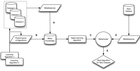
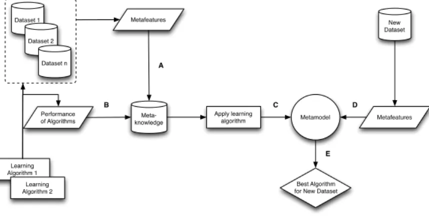
Figure 2.1 illustrates a step by step MtL framework for algorithm selection. The process starts with a collection of datasets and learning algorithms. For each of those datasets, we extract metafeatures that describe their
characteris-tics (A). Then, each algorithm is tested on each dataset and its performance is
estimated (B). The metafeatures and the estimates of performance are stored
meta-2.6. METALEARNING 23 learner) that induces a meta-model that relates the values of the metafeatures
with the best algorithm for each dataset (C). Given the metafeatures of a new
dataset (D), this meta-model is used to recommend one or more algorithm for
that dataset (E). Dataset 1 Dataset 2 Dataset n Learning Algorithm 1 Learning Algorithm 2 Meta-knowledge Apply learning algorithm Metamodel New Dataset Metafeatures Best Algorithm for New Dataset Performance of Algorithms Metafeatures A B C D E
Figure 2.1: Metalearning framework for algorithm recommendation.
2.6.1
Metadata
Generating the metadata is the most important step in a MtL process. Besides choosing the appropriate metatarget for the task, it is crucial to select
mean-ingful metafeatures that contain information to successfully achieve the main
goal. We provide a more in-depth discussion on metafeatures in section 3.2 of this thesis.
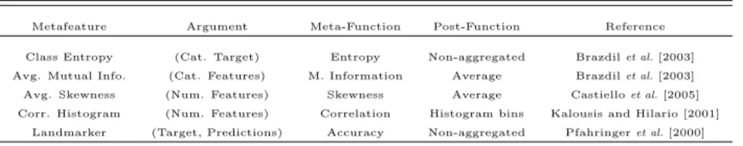
Metafeatures can be divided into three types (Figure 2.2):
• Simple, statistical and information-theoretic. These are the most common type of metafeatures extracted using descriptive statistics and information-theoretic measures. Some examples: number of features/examples, num-ber of instances with missing values (simple); mean skewness of numeric features, mean value of correlation (statistical); class entropy, mutual information for symbolic features (information-theoretic). We refer the
reader to the following papers for more examples: [K¨opfet al., 2000; Gama
and Brazdil, 1995].
of the induced model. For example, the number of leaf nodes in a decision
tree [Peng et al., 2002a] or mean of the off-diagonal values of a kernel
matrix in a Support Vector Machines model [Soares and Brazdil, 2006].
• Landmarkers. This type of metafeatures are quick estimates of an al-gorithm’s performance. They can be obtained in three different ways: through the run of simplified versions of an algorithm (for instance, a
deci-sion stump [Bensusan and Giraud-Carrier, 2000; Pfahringeret al., 2000]);
quick performance estimates on a sample of the data, also called
sub-sampling landmarkers [F¨urnkranz and Petrak, 2001]; and finally, through
an ordered sequence of sub-sampling landmarkers for a single algorithm, which allows to form the so called learning curve of an algorithm. In this case, not only the estimates can be used as metafeatures but also the shape of the curve [Leite and Brazdil, 2005].
Datasets Datasets Datasets Simple, statistical and information-theoretic Model-based Learning Learning Model Performance Estimates Landmarkers Model
Figure 2.2: Metafeatures taxonomy. Source: Brazdilet al.[2009].
Brazdilet al.[2009] defined three fundamental issues that every metafeature
2.6. METALEARNING 25
• Discriminative power. The metafeatures need to contain information that distinguishes between the base-algorithms in terms of their performance.
• Computational complexity. The computation of the metafeatures should not be too demanding. If not, it may not compensate generating a MtL system if one can save resources by exploring all the hypotheses for a
given learning problem. Pfahringer et al.[2000] suggested that the
com-putational complexity of extracting metafeatures should be at mostO(n
logn).
• Dimensionality. Given that the number of meta-examples of a MtL prob-lem is usually small, the number of metafeatures should not be too large or overfitting may occur. Kalousis and Hilario [2001] found evidence that feature selection can improve a MtL process which supports this claim. Each example in a meta-dataset represents a learning problem. As in other learning task, MtL needs a satisfactory number of examples in order to induce a reliable model. The number of meta-examples is often seen as a problem for
MtL [Brazdilet al., 2009]. Soares [2009] proposed a framework that enables to
tackle this problem by generating different versions of a dataset through changes in the role of features/target.
Concerning the development of a MtL system, the first decision that must
be made is about the type ofmetatarget, in other words, the dependent variable
of the meta-level learning process. This variable can take several forms depend-ing on the main goal of the MtL system and the nature of the base-level task (i.e., classification, regression or other). The most simple form of metatarget is a classification scheme (binary or multi-class, depending on the number of algorithms) in which for a given dataset, the metamodel predicts the class that represents the algorithm with better performance from a set. The great disad-vantage of this type of metatarget is if the metamodel fails its prediction, the costs can be very high.
Another type of metatarget, instead of a single recommendation, is the sug-gestion of a subset of algorithms. Given the algorithm with expected best performance, a heuristic measure can be defined to indicate the algorithms that also perform well in comparison with the best algorithm. Typically, these
meta-models are induced with rules or Inductive Logic Programming [Kalousis and Theoharis, 1999].
Predicting a subset of algorithms provides several recommendations for the user. However, they are not ordered. This can negatively influence the data mining process. Therefore, algorithm recommendation in form of rankings seems a good alternative. A MtL method that provides recommendations in the form
of rankings is proposed in the paper by Brazdilet al.[2003]. The system includes
an adaptation of the k-nearest neighbours algorithm that identifies algorithms which are expected to tie, providing a reduced ranking by only including one of them in the recommendation.
Finally, if one is interested in concrete value regarding the performance of an algorithm in a dataset and not the actual relative performance of a set of algo-rithms, the metatarget can be defined as estimates of performance. In this case, the MtL problem takes the form of a regression, one for each base-algorithm. Besides that this type of metafeature provides more detailed information to the user, it also allows to transform the output of the metamodels in one of the previous recommendations forms mentioned above.
2.6.2
Applications
[Lemkeet al., 2015] identified in the literature a multiple use of the term MtL
for distinct concepts, specifically:
• Ensemble methods and combination of base-learners. Algorithms for com-bination of base-models, such as bagging, boosting or stacking, are often regarded as MtL.
• Algorithm recommendation. Probably the area for which has been devoted the largest amount of MtL research. Most systems attempt to learn a relationship between data characteristics and algorithm performance.
• Dynamic bias selection. In this area, MtL algorithms are mostly de-signed for bias management and detecting concept drifts, typically in data streams environments.
2.6. METALEARNING 27 transfer knowledge across multiple related domains or tasks, and therefore accumulate experience that can be useful in future tasks.
• Metalearning systems. This area regards the development of systems that automate specific tasks of a data scientist or provide assistance in those tasks.
We follow this organization to give an overview of the state-of-the-art for the main applications in each topic.
Ensemble methods
We already mentioned algorithms such as bagging, boosting and stacking in the section 2.2 of this thesis, so we refer the reader to that section to avoid repetition.
Algorithm recommendation
As mentioned before, Rendellet al.[1987] and Rendell and Cho [1990] published
the first papers in which the expression ”meta-learning” is used in Machine Learning. In the former, they proposed the Variable Bias Management System (VBMS). Here, the problem of algorithm recommendation is studied for the first time and the need for methods that develop models with different biases is identified. However, the experiment is rather preliminary: only the execution time of the algorithms is considered, the type of metafeatures is very simple (for instance, number of examples) and the evaluation carried is insufficient. In the latter, the data characterization was more detailed and set roots for the MtL research in following years, boosted by the already mentioned European projects, StatLog and METAL.
In the StatLog project, besides great developments in the scope of data char-acterization [Gama and Brazdil, 1995], MtL was used to predict the applicability
of learning algorithms to a given data set [Brazdilet al., 1994]. By applicability
understand the notion of assessing if the performance of one learning algorithm is significantly different from the best algorithm on the corresponding dataset. The METAL project allowed to develop the research on MtL focusing more on
More recently, Sun and Pfahringer [2013] addressed this problem by proposing the Pairwise meta-rules (a new high-level framework to generate metafeatures) and the ART forests algorithm (a ranking algorithm based on Random Forests).
Kalousiset al.[2004] published a very interesting paper in which the authors
looked for similarities between algorithms by means of error correlation, and similarities between datasets based on patterns of error correlation and relat
![Figure 2.2: Metafeatures taxonomy. Source: Brazdil et al. [2009].](https://thumb-us.123doks.com/thumbv2/123dok_us/486691.2557632/49.892.263.708.572.1009/figure-metafeatures-taxonomy-source-brazdil-al.webp)