High-Dimensional Non-Gaussian Data Clustering using Variational Learning of Mixture Models

(1)

High-Dimensional Non-Gaussian Data

Clustering using Variational Learning of

Mixture Models

Wentao Fan

A Thesis in

Department of Electrical and Computer Engineering

Presented in Partial Fulﬁllment of the Requirements

for the Degree of Doctor of Philosophy (Electrical and Computer Engineering) at Concordia University

Montr´eal, Qu´ebec, Canada

December 2013

c

(2)

CONCORDIA UNIVERSITY SCHOOL OF GRADUATE STUDIES This is to certify that the thesis prepared

By: Wentao Fan

Entitled: High-DimensionalNon-Gaussian Data Clustering using Variational Learning of Mixture Models

and submitted in partial fulfillment of the requirements for the degree of

DOCTOR OF PHILOSOPHY (Electrical & Computer Engineering)

complies with the regulations of the University and meets the accepted standards with respect to originality and quality.

Signed by the final examining committee:

Chair Dr. F. Haghighat External Examiner Dr. G.-A. Bilodeau External to Program Dr. P. Grogono Examiner Dr. A. Ben Hamza Examiner Dr. A. Youssef Thesis Supervisor Dr. N. Bouguila Approved by Chair of Department or Graduate Program Director Dr. A.R. Sebak,Graduate Program Director

December 11, 2013

(3)

Abstract

High-Dimensional Non-Gaussian Data Clustering using

Variational Learning of Mixture Models

Wentao Fan, Ph.D.

Concordia University, 2013

Clustering has been the topic of extensive research in the past. The main concern is to automat-ically divide a given data set into different clusters such that vectors of the same cluster are as sim-ilar as possible and vectors of different clusters are as different as possible. Finite mixture models have been widely used for clustering since they have the advantages of being able to integrate prior knowledge about the data and to address the problem of unsupervised learning in a formal way. A crucial starting point when adopting mixture models is the choice of the components densities. In this context, the well-known Gaussian distribution has been widely used. However, the deploy-ment of the Gaussian mixture implies implicitly clustering based on the minimization of Euclidean distortions which may yield to poor results in several real applications where the per-components densities are not Gaussian. Recent works have shown that other models such as the Dirichlet, generalized Dirichlet and Beta-Liouville mixtures may provide better clustering results in appli-cations containing non-Gaussian data, especially those involving proportional data (or normalized histograms) which are naturally generated by many applications. Two other challenging aspects that should also be addressed when considering mixture models are: how to determine the model’s complexity (i.e. the number of mixture components) and how to estimate the model’s parameters. Fortunately, both problems can be tackled simultaneously within a principled elegant learning framework namely variational inference. The main idea of variational inference is to approximate the model posterior distribution by minimizing the Kullback-Leibler divergence between the exact (or true) posterior and an approximating distribution. Recently, variational inference has provided good generalization performance and computational tractability in many applications including learning mixture models.

(4)

In this thesis, we propose several approaches for high-dimensional non-Gaussian data cluster-ing based on various mixture models such as Dirichlet, generalized Dirichlet and Beta-Liouville. These mixture models are learned using variational inference which main advantages are com-putational efficiency and guaranteed convergence. More specifically, our contributions are four-fold. Firstly, we develop a variational inference algorithm for learning the finite Dirichlet mixture model, where model parameters and the model complexity can be determined automatically and simultaneously as part of the Bayesian inference procedure; Secondly, an unsupervised feature selection scheme is integrated with finite generalized Dirichlet mixture model for clustering high-dimensional non-Gaussian data; Thirdly, we extend the proposed finite generalized mixture model to the infinite case using a nonparametric Bayesian framework known as Dirichlet process, so that the difficulty of choosing the appropriate number of clusters is sidestepped by assuming that there are an infinite number of mixture components; Finally, we propose an online learning framework to learn a Dirichlet process mixture of Beta-Liouville distributions (i.e. an infinite Beta-Liouville mixture model), which is more suitable when dealing with sequential or large scale data in contrast to batch learning algorithm. The effectiveness of our approaches is evaluated using both synthetic and real-life challenging applications such as image databases categorization, anomaly intrusion detection, human action videos categorization, image annotation, facial expression recognition, behavior recognition, and dynamic textures clustering.

(5)

Acknowledgements

First, I would like to express my greatest gratitude to my supervisor, Dr. Nizar Bouguila for opening the door of the academic world to me. Within six years, from my Master to Ph.D. study, he has always been a wonderful advisor, mentor and motivator. I learned a lot from his valuable tutoring, not only technical knowledge but also about dealing in real life. I will be always grateful to him for his support and persistent encouragement.

Special thanks goes to Dr. A. Ben Hamza for his patience and guidance through my INSE6510 project. I also beneﬁt a lot from being his teaching assistant for the course Comp471.

It is a great pleasure to work with the former and current colleagues in our lab. I would like to thank them for their helpful suggestions and discussions during my research. I am lucky to share six years’ time with them.

I would like to thank Fonds de recherche du Qu´ebec-Nature et technologies (FQRNT) for the scholarship at the doctorate-level. I am also grateful to the Faculty of Engineering and Computer Science of Concordia University for the Special Scholarship for New High Caliber Ph.D. Stu-dents. In addition, I would like to express my gratitude to the Chinese government for the Chinese Government Award for Outstanding Self-ﬁnanced Students Abroad.

Last, but by no means least I would like to thank my family for their love and support in all my years, and especially my wife for her love, encouragement and endless patience with me.

(6)

List of Tables

2.1 Parameters of the different generated data sets. N denotes the total number of elements,nj denotes the number of elements in clusterj. αj1,αj2, αj3andπj are

the real parameters.α_ˆj1,αˆj2,αˆj3andπˆjare the estimated parameters by variational

inference. α_˘j1, α˘j2, α˘j3 and π˘j are the estimated parameters using DM. We can

observe that both algorithms are able to estimate unknown parameters, yet the variational algorithm always gives more accurate values. . . 18 2.2 Rum time (in seconds) and number of iterations required before convergence for

varDM and DM. . . 22 2.3 Clustering Accuracies with varDM Model and varGM Model. M∗ denotes the

average number of clusters. . . 22 2.4 Average Rounded Confusion Matrix using the varDM Model to categorize Data

Set A. . . 24 2.5 Average Rounded Confusion Matrix using the varDM Model to categorize Data

Set B. . . 25 2.6 Confusion Matrix for Intrusion Detection with Variational Dirichlet Mixture Model. 26 2.7 Intrusion Detection Results Using different approaches. . . 26 3.1 Parameters of the different generated data sets. N denotes the total number of

elements,nj denotes the number of elements in clusterj for the relevant features.

αj1,βj1,αj2,βj2,αj3,βj3 andπj are the real parameters of the mixture models of

relevant features. α_ˆj1, βˆj1, αˆj2, βˆj2, αˆj3, βˆj3 andπˆj are the estimated parameters

from variational inference. . . 34 3.2 The average classiﬁcation accuracy and the number of components (Mˆ) computed

on the KTH data set using varFsGD, MMLFsGD, varGD and varFsGau over 30 random runs. . . 39 4.1 Parameters of the generated data sets. N denotes the total number of elements,Nj

denotes the number of elements in clusterj. αj1, αj2, βj1,βj2 andπj are the real

parameters. α_ˆj1,αˆj2,βˆj1,βˆj2 andπˆj are the estimated parameters by the proposed

algorithm. . . 53 4.2 The average classiﬁcation accuracy and the number of categories (Mˆ) computed

by different algorithms for the Caltech data set. . . 59 4.3 The average classiﬁcation accuracy computed by different algorithms. . . 62

(10)

4.4 Performance evaluation on the automatic annotation system based on different cat-egorization methods. . . 63 4.5 Sample annotation results by usingInFsGDclassiﬁcation method. . . 64 4.6 The comparison of image retrieval performance. . . 64 5.1 The average recognition accuracy (_%) and the number of categories (M) computed

by different algorithms for the JAFFE data set. The numbers in parenthesis are the standard deviations of the corresponding quantities. . . 78 5.2 The average recognition accuracy rate (Acc) and the average estimated number of

categories (M) computed using different algorithms on the three data sets: facial expression (face), mouse behavior (mouse) and human activity (UCF11). . . 79 5.3 The average accuracy and the number of categories (M) computed by different

(11)

List of Figures

2.1 Graphical model representation of the ﬁnite Dirichlet mixture. Symbols in circles denote random variables; otherwise, they denote model parameters. Plates indicate repetition (with the number of repetitions in the lower right), and arcs describe conditional dependencies between variables. . . 13 2.2 Mixture densities for the synthetic data sets. (a) Data set 1, (b) Data set 2, (c) Data

set 3, (d) Data set 4, (e) Data set 5, (f) Data set 6. . . 19 2.3 Variational likelihood bound for each iteration for the different generated data sets.

The initial number of components is 15. Vertical dash lines indicate cancelation of components. (a) Data set 1, (b) Data set 2, (c) Data set 3, (d) Data set 4, (e) Data set 5, (f) Data set 6. . . 20 2.4 Variational likelihood bound as a function of the ﬁxed assumed number of mixture

components for the different generated data sets. (a) Data set 1, (b) Data set 2, (c) Data set 3, (d) Data set 4, (e) Data set 5, (f) Data set 6. . . 21 2.5 Sample images from each group of sports event data set: (a) Rowing. (b)

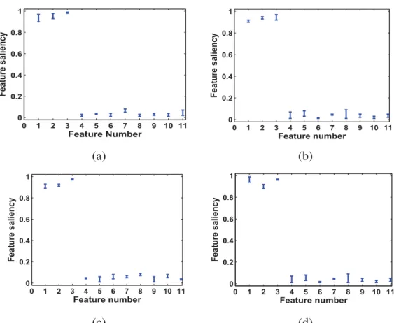
Bad-minton. (c) polo. (d) Bocce. (e) Snow Boarding. (f) Croquet. (g) Sailing. (h) Rock climbing. . . 23 3.1 Feature saliency for synthetic data sets with one standard deviation over ten runs.

(a) Data set 1, (b) Data set 2, (c) Data set 3, (d) Data set 4. . . 35 3.2 Examples of frames, representing different human actions in different scenarios,

from video sequences in the KTH data set. . . 36 3.3 Confusion matrix for the KTH data set. . . 39 3.4 (a) Classiﬁcation accuracy vs. vocabulary size for the KTH data set; (b)

Classiﬁ-cation accuracy vs. the number of aspects for the KTH data set. . . 40 3.5 Feature saliencies of the different aspect features over 30 runs for the KTH data set. 41 4.1 Graphical model representation of the inﬁnite GD mixture model with feature

se-lection. Symbols in circles denote random variables; otherwise, they denote model parameters. Plates indicate repetition (with the number of repetitions in the lower right), and arcs describe conditional dependencies between variables. . . 48 4.2 Mixing probabilities of components, πj, found for each synthetic data set after

convergence. (a) Data set 1, (b) Data set 2, (c) Data set 3, (d) Data set 4. . . 55 4.3 Features saliencies for synthetic data sets with one standard deviation over ten runs.

(12)

4.4 Sample images from the four categories of the Caltech data set. . . 57 4.5 Sample segmentation results from the four categories of the Caltech data sets . . . 58 4.6 (a) Classiﬁcation accuracy vs. the number of aspects; (b) Feature saliency for each

aspect. . . 59 5.1 Sample images from the JAFFE data set: (a) Anger, (b) Disgust, (c) Fear, (d)

Happiness, (e) Sadness, (f) Surprise, (g) Neutral. . . 77 5.2 Confusion matrix obtained byOIBLMfor the JAFFE data set. . . 79 5.3 Sample frames from the each data set. (a): facial expression; (b): mouse behavior;

(c): human action. . . 80 5.4 Performance comparison on the three data sets: facial expression, mouse behavior

and human activity using different algorithms. . . 82 5.5 Sample fames from the DynTex data set. . . 83 5.6 Confusion matrix obtained byOIBLMfor the DynTex data set. . . 84 5.7 Performance comparison in terms of classiﬁcation accuracy provided different

(13)

Chapter 1

Introduction

1.1

Clustering via Finite Mixture Models

Data clustering is the unsupervised partitioning of data into homogeneous components. It is an important problem in several fields, such as signal and image processing, and has been the topic of extensive research in the past [1–4]. There are a myriad of clustering methods (see [5] for a review). Among all these methods, finite mixture models have been shown to provide flexibility for data clustering [6] and have been successfully applied in several domains and applications. Examples include cognitive understanding [7], epidemiological studies [8], speaker’s location detection [9], person authentication [10], and so forth. Indeed, they have been proven to be a powerful way to capture hidden structure in data and to take uncertainty into account.

A finite mixture model is formed by taking linear combinations of a finite number of basic distributions. These basic distributions are called components of the mixture model. For instance, a finite mixture model withM components is given by

p₍X_{) =}

M

j=1

πjp(X|θj) (1.1)

wherep₍X|θj)is a component of the mixture and has its own parameter θj. In general, mixture

models can comprise linear combinations of any distributions, such as Gaussian, Beta, Dirichlet, etc. The parameters {πj} are called mixing coefﬁcients and are subject to the constraints: 0 ≤

πj ≤ 1 and

M

j=1πj = 1. In mixture modeling, three challenging aspects should be carefully

addressed: how to choose the proper basic distribution, how to estimate the model’s parameters and how to select the model’s complexity. Each of these aspects has a signiﬁcant impact on the performance of model learning.

(14)

Selecting the most accurate probability density functions (pdfs) that best represent the mixture components is important when modeling and clustering data. The Gaussian assumption has been widely adopted (i.e. assuming that each per-class density is Gaussian) due to its simplicity. In several real-world applications, however, when the data clearly appear with a non-Gaussian struc-ture, this assumption fails. For instance, recent works have shown that other models such as the Dirichlet [11–16], the generalized Dirichlet [17–23] and the Beta-Liouville mixtures [24–27] pro-vide better clustering results in several applications, especially those involving normalized count data (i.e. proportional vectors) which naturally appear in many applications such as text, image and video modeling.

The majority of parameter estimation approaches in mixture modeling consider either de-terministic or Bayesian techniques [6]. Dede-terministic techniques aim at optimizing the model likelihood function, are generally implemented within the expectation-maximization (EM) [28] framework, and are well documented [29, 30]. On the other hand, Bayesian techniques have been proposed to avoid drawbacks related to deterministic techniques such as their suboptimal gener-alization performance, dependency on initigener-alization, over-ﬁtting and noise level under-estimation problems of classic likelihood-based inference [31, 32]. These drawbacks are avoided via the incor-poration of prior knowledge (or belief) in a principled way and then marginalizing over parameter uncertainty. Bayesian methods [33, 34] have considered either Laplace’s approximation [35] or

Markov chain Monte Carlo (MCMC) simulation techniques [36, 37]. While MCMC techniques are computationally expensive, Laplace’s approximation is generally imprecise, since it is based on the strong assumption that the likelihood function is unimodal which is not generally the case for finite mixtures of distributions [38]. Recently,Variational inference(also known asvariational Bayes) [39, 40] framework has been widely used as an efficient alternative and as a more control-lable way to approximate Bayesian learning. The variational learning approach was introduced in the context of the multi-layer perceptron in [41] where it was called ensemble learning and de-veloped further in [42, 43]. The main idea is to approximate the model posterior distribution by minimizing the Kullback-Leibler divergence between the exact (or true) posterior and an approxi-mating distribution. The variational inference has received a lot of attention and has provided good generalization performance and computational tractability in various applications including finite

(15)

mixtures learning [44–46]. For instance, the authors in [39, 40, 47, 48] have developed comprehen-sive frameworks for variational learning, in the case of Gaussian mixture models, which have been shown to provide better parameter estimates than themaximum likelihood(ML) approach.

Another crucial issue when using mixture models is the model complexity (i.e. model structure or number of mixture components) determination problem. Indeed, it is important to estimate the number of clusters that best describes the data without over-fitting or under-fitting it [6]. In general, this problem is tackled using ML method in conjunction with a given model selection criterion, such as minimum description length (MDL) and minimum message length (MML) [6, 11], in fre-quentist frameworks or by considering Bayes factors in the case of fully Bayesian approaches. However, these approaches are clearly time-consuming since they have to evaluate a given selec-tion criterion for several numbers of mixture components. This is especially true in the case of the Bayesian approach because it requests the evaluation of multi-dimensional integrals which is generally tackled via MCMC techniques (e.g. Gibbs sampling, Metropolis Hastings). Despite the fact that MCMC techniques have revolutionized Bayesian statistics by accommodating situations characterized by uncertainty of the statistical model structure [49–51], their use is often limited to small-scale problems in practice because of its high computational cost and the difficulty in tracking convergence. Apart from the elegant way to estimate the parameters of mixture models, another advantage of variational inference is that it is able to automatically determine the number of mixture components as part of the Bayesian inference procedure.

Data clustering is known to be a challenging task in modern knowledge discovery and data mining. This is especially true in high-dimensional spaces mainly because of data sparsity. Thus, feature selection is a crucial factor to improve the clustering performance [52–54]. Its primary objective is the identification and the reduction of the influence of extraneous (or irrelevant) fea-tures which do not contribute information about the true clusters structure. The automatic selection of relevant features in the context of unsupervised learning is challenging and is far from trivial because inference has to be made on both the selected features and the clustering structure [54– 61]. [54] is an early influential paper advocating the use of finite mixture models for unsupervised feature selection. The main idea is to suppose that a given feature is generated from a mixture of two univariate distributions. The first one is assumed to generate relevant features and is different

(16)

for each cluster and the second one is common to all clusters (i.e. independent from class labels) and assumed to generate irrelevant features1_{. The unsupervised feature selection models in [54, 60]}

have been trained using a MML objective function with the EM algorithm. Despite the fact that the EM algorithm is the procedure of choice for parameter estimation in the case of incomplete data problems where part of the data is hidden, several studies have shown theoretically and exper-imentally that the EM algorithm, in deterministic settings (e.g. ML estimation), converges either to a local maximum or to a saddle point solution and depends on an appropriate initialization (see, for instance, [29, 63, 64]) which may compromise the modeling capabilities. Recently, variational inference have shown promising results in learning mixture models with integrated unsupervised feature selection [57, 65], by providing parameters estimation and features selection in a single optimization framework.

1.2

Variational Inference

In this section, a brief introduction to variational inference is presented. Assume that we have a fully Bayesian model in which all parameters are given proper prior distributions. Let Θ repre-sents the set of all non-observed variables (including latent variables) and X denotes the set of observations. The goal of variational inference is to ﬁnd a proper approximationq₍Θ₎for the true posterior distributionp₍Θ|X₎. In order to do this, we can write the following decomposition of the log marginal probability of the observed dataX, which holds for any choice of distributionq₍Θ₎

lnp₍X_{) =}L₍q_{) +}KL₍q||p₎ (1.2) where L(q_{) =} q₍Θ_{) ln} p(Θ,X) q₍Θ₎ dΘ (1.3) KL(q||p_{) =} − q₍Θ_{) ln} p(Θ|X) q₍Θ₎ dΘ (1.4)

here,KL₍q||p₎is the Kullback-Leibler (KL) divergence which represents the dissimilarity between the true posteriorp₍Θ|X₎and the variational approximationq₍Θ₎. We know that KL₍q||p₎ ≥ ₀

1_{Several other quantitative formalisms for relevance in the case of feature selection have been proposed in the past}

(17)

(according to Jensen’s inequality), and that the equality is achieved when if and only ifq₍Θ_{) =} p₍Θ|X₎. Then, we can conclude thatL₍q₎≤_lnp₍X₎from Eq. (1.2), which means thatL₍q₎forms a lower bound on_lnp₍X₎.

Suppose that we allow any possible choice for q₍Θ₎. Then, the lower bound of _lnp₍X₎

can be maximized with respect to q₍Θ₎ when the KL divergence is minimized, that is when

q₍Θ_{) =} p₍Θ|X₎. However, in practice the true posterior distribution is normally computation-ally intractable and can not be directly used for variational inference. Thus, a restricted family of distributionsq₍Θ₎needs to be considered. An ideal restriction should have the property that, the family ofq₍Θ₎comprises only tractable distributions, and at meanwhile is still flexible enough to provide a good approximation to the true posterior distribution. A common approach in variational inference literatures is to adopt factorization assumptions for restricting the form of q₍Θ₎ [66]. This approximation framework is known asmean field theory[67, 68] which was developed in the filed of physics [69]. With the factorization assumption, the posterior distribution q₍Θ₎ can be factorized intoT disjoint tractable distributions as

q₍Θ_{) =}

T

i=1

qi(Θi) (1.5)

Notice that this is the only assumption about the distribution, and no further restriction is placed on the functional forms of the individual factorsqi(Θi). In order to maximize the lower boundL(q),

we need to make a variational optimization ofL₍q₎with respect to each of the distributionsqi(Θi)

(18)

then the optimization ofL₍q₎with respect to a speciﬁc factorqs(Θs)can be given as L(q₎₌ T i=1 qiln p₍Θ,X₎ T i=1qi dΘ = qs T i=s qi lnp₍Θ,X₎− T i=1 lnqi dΘ = qs T i=s qilnp(Θ,X)dΘi dΘs− qslnqsdΘs+const. = qslnf(Θs,X)dΘs− qslnqsdΘs+const. (1.6) where any terms that are independent of qs(Θs)are absorbed into the additive constant. A new

distributionf₍Θs,X)in Eq. (1.6) is introduced as

lnf₍Θs,X) =

T

i=s

qilnp(Θ,X)dΘi =lnp(Θ,X)i=s (1.7)

Here, we use the notation . . .i=s to represent the expectation with respect to all the

distribu-tions of qi(Θi) except for i = s. We can also notice that Eq. (1.6) is actually a minus KL

di-vergence betweenqs(Θs) andf(Θs,X). Therefore, maximizing L(q)in Eq. (1.6) is equivalent

to minimizing the KL divergence. We know that the KL divergence reaches its minimum when

qs(Θs) =f(Θs,X). Thus, a general expression for the optimal solutionqs∗(Θs)can be given by

lnqs∗(Θs) =lnp(X,Θ)i=s+const. (1.8)

Here, the additive constant denotes the normalization coefﬁcient for the distribution. By taking the exponential of both sides of Eq. (1.8) and normalize, we can obtain the variational solution of

q∗s(Θs)as q_s∗₍Θs) = explnp₍X,Θ₎i=s explnp₍X,Θ₎i=s dΘ (1.9)

Since the expression forq∗_s₍Θs)depends on calculating the expectations with respect to the other

(19)

lower bound. In general, in order to perform the variational inference, all the factorsqi(Θi)need

to be suitably initialized ﬁrst, then each factor is updated in turn with a revised value obtained by Eq. (1.9) using the current values of all of the other factors. Convergence is guaranteed since bound is convex with respect to each of the factorsqi(Θi)[66, 70].

1.3

Contributions

The goal of this thesis is to propose several novel approaches for high-dimensional non-Gaussian data clustering based on variational inference framework in the context of various mixture models including Dirichlet, generalized Dirichlet and Beta-Liouville. The contributions of this thesis are listed as the following:

Finite Dirichlet Mixture Models with Variational Bayes Learning:

We propose a variational inference framework for learning finite Dirichlet mixture models. Compared with other algorithms which are commonly used for mixture models (such as EM), our approach has several advantages: first, the problem of over-fitting is prevented; furthermore, the complexity of the mixture model (i.e. the number of components) can be determined automatically and simultaneously with the parameters estimation as part of the Bayesian inference procedure; finally, since the whole inference process is analytically tractable with closed-form solutions, it may scale well to large applications.

Finite Generalized Dirichlet Mixture Models with Unsupervised Feature Selection:

A variational inference framework is developed for unsupervised non-Gaussian feature se-lection, in the context of ﬁnite generalized Dirichlet mixture-based clustering. Under the proposed principled variational framework, we simultaneously estimate, in a closed-form, all the involved parameters and determine the complexity (i.e. both model an feature selec-tion) of the ﬁnite generalized Dirichlet mixture model.

Inﬁnite Generalized Dirichlet Mixture Models via Dirichlet Process:

We extend the finite generalized Dirichlet mixture model to an infinite case through a non-parametric Bayesian framework namely Dirichlet process. The infinite assumption is used

(20)

to avoid problems related to model selection (i.e. determination of the number of clusters) and allows simultaneous separation of data in to similar clusters and selection of relevant features.

Online Learning of Inﬁnite Beta-Liouville Mixture Models:

We propose a novel online clustering approach based on a Dirichlet process mixture of Beta-Liouville distributions (i.e. an inﬁnite Beta-Beta-Liouville mixture model). We are mainly moti-vated by the fact that online algorithms allow data instances to be processed in a sequential way, which is important for large-scale and real-time applications.

1.4

Thesis Overview

The organization of this thesis is as follows:

J Chapter 1 introduced the background knowledge regarding ﬁnite mixture models and varia-tional inference learning framework.

J In Chapter 2, we propose a variational inference framework approach to learn ﬁnite Dirichlet mixture models. Both synthetic and real data, generated from real-life challenging applica-tions namely image databases categorization and anomaly intrusion detection, are experi-mented to verify the effectiveness of the proposed approach. This work has been published in theIEEE Transactions on Neural Networks and Learning Systems[71].

J In Chapter 3, we develop a novel statistical approach of simultaneous clustering and feature selection for unsupervised learning. The proposed approach is based on ﬁnite generalized mixture models and variational inference learning. We apply the proposed approach to both synthetic data and a challenging application which concerns human action videos catego-rization. This contribution has been published in theIEEE Transactions on Knowledge and Data Engineering[72].

J In Chapter 4, we propose a novel unsupervised clustering approach based on an inﬁnite generalized mixture model with variational framework. We test the proposed approach using

(21)

both synthetic data and real-world applications involving visual scenes categorization, auto-annotation and retrieval. This research work has been published inPattern Recognition[73]. J In Chapter 5, a novel online clustering approach based on inﬁnite Beta-Liouville mixture models is proposed. The effectiveness of the proposed work is evaluated on three challenging real applications namely facial expression recognition, behavior modeling and recognition, and dynamic textures clustering. This work has been published in theIEEE Transactions on Neural Networks and Learning Systems[74].

(22)

Chapter 2

Variational Learning for Finite Dirichlet Mixture

Models

In this chapter, we focus on the variational learning of finite Dirichlet mixture models. Com-pared to other algorithms which are commonly used for mixture models (such as expectation-maximization), our approach has several advantages: first, the problem of over-fitting is prevented; furthermore, the complexity of the mixture model (i.e. the number of components) can be de-termined automatically and simultaneously with the parameters estimation as part of the Bayesian inference procedure; finally, since the whole inference process is analytically tractable with closed-form solutions, it may scale well to large applications. Both synthetic and real data, generated from real-life challenging applications namely image databases categorization and anomaly intrusion detection, are experimented to verify the effectiveness of the proposed approach.

2.1

The Finite Dirichlet Mixture Model

The Dirichlet distribution is the multivariate generalization of the Beta distribution, which offers considerable flexibility and ease of use. In contrast to Gaussian distribution which only contains symmetric modes, the Dirichlet distribution may have multiple symmetric and asymmetric modes. Additionally, the Dirichlet distribution is defined in the compact support_[0,_1]and can be easily generalized to be defined in a compact support of the form_[A, B_], where₍A, B₎ ∈ R2. Thus, the Dirichlet distribution is a better choice for modeling compactly supported data, such as images, text or videos [11].

(23)

A ﬁnite mixture of Dirichlet distributions withM components is represented by [75] p₍X|π, α_{) =} M j=1 πjDir(X|αj) (2.1)

where π _{= (}π₁, . . . , πM) denotes the mixing coefﬁcients which are positive and sum to one.

Dir(X|αj)in Eq. (2.1) is the Dirichlet distribution of componentjwith its own positive parameters

αj = (αj1, . . . , αjD), and is deﬁned by:

Dir(X|αj) = Γ( D l=1αjl) D l=1Γ(αjl) D l=1 Xαjl−1 l (2.2) whereX _{= (}X₁, . . . , XD)and D

l=1Xl = 1,0 ≤ Xl ≤1forl = 1, . . . , D. It is noteworthy that

the Dirichlet distribution is used here as a parent distribution to model directly the data and not as a prior to the multinomial.

Consider a set of N independent identically distributed vectorsX ₌ {X₁, . . . , XN}assumed

to be generated from the mixture distribution in Eq. (2.1), the likelihood function of the Dirichlet mixture model is given by

p₍X |π, α_{) =} N i=1 M j=1 πjDir(Xi|αj) (2.3) It is convenient to interpret the ﬁnite Dirichlet mixture model in Eq. (2.1) as a latent variable model. Thus, for each vector Xi, we introduce a M-dimensional binary random vector Zi = {Zi1, . . . , ZiM}, such thatZij ∈ {0,1},

M

j=1Zij = 1andZij = 1ifXi belongs to componentj

and₀, otherwise. The latent variablesZ ₌{Z₁, . . . , ZN}are actually hidden variables, so that do

not appear explicitly in the model. The conditional distribution ofZ given the mixing coefﬁcients

πis deﬁned as p₍Z|π_{) =} N i=1 M j=1 πZij j (2.4)

Then, the likelihood function with latent variables, which is actually the conditional distribution of data setX given the class labelsZ, can be written as

p₍X |Z, α_{) =} N i=1 M j=1 Dir(Xi|αj)Zij (2.5)

(24)

Having the data setX, an important problem is the learning of the mixture parameters. By learning, we mean both the estimation of the parameters and the selection of the number of componentsM. In the following, we describe a variational inference approach, for ﬁnite Dirichlet mixture models, that can handle these two issues simultaneously.

2.2

Variational Inference for Finite Dirichlet Mixture Model

2.2.1

Variational Approximation

In order to estimate the parameters of the finite Dirichlet mixture model and to select the number of components correctly, we adopt the variational inference methodology proposed in [47] for finite Gaussian mixtures. The main idea of this framework is based on the estimation of the mixing coefficientsπby maximizing the marginal likelihoodp₍X |π₎given by

p₍X |π_{) =}

Z

p₍X,Z, α|π₎dα (2.6)

wherep₍X,Z, α|π₎is the joint distribution of all the mixture model random variables conditioned on the mixing coefﬁcients as

p₍X,Z, α|π_{) =} p₍X |Z, α₎p₍Z|π₎p₍α₎ (2.7) An important step now is to deﬁne a conjugate priorp₍α₎over theαparameters. Since the Dirichlet belongs to the exponential family of distributions [76], a conjugate prior can be derived as follows [77]: p₍αj) =f(ν, λ) Γ(Dl=1αjl) D l=1Γ(αjl) νD l=1 e−λl(αjl−1) _(2.8)

where f₍ν, λ₎ is a normalization coefficient and₍ν, λ₎ are hyperparameters. Unfortunately, this formal conjugate prior for the Dirichlet distribution is intractable, mainly because of the diffi-culty to evaluate the normalization coefficient, and cannot be applied for the variational inference directly as it shall be clearer later. We decided, faut de mieux, to tackle this problem in a sim-ilar way as in [78] where the authors proposed a conjugate prior for the Beta distribution (i.e.

(25)

one-dimensional Dirichlet) within a variational framework. Indeed, we assume that the Dirich-let parameters are statistically independent and for each parameterαjl, the Gamma distribution is

adopted to approximate the conjugate prior as

p₍αjl) =G(αjl|ujl, vjl) = vujl jl Γ(ujl) αujl−1 jl e− v_jlα_jl (2.9) whereujlandvjl are hyperparameters, subject to the constraintsujl > 0andvjl > 0. Therefore,

we have p₍α_{) =} M j=1 D l=1 p₍αjl) (2.10)

By substituting Eqs. (2.4), (2.5) and (2.10) into Eq. (2.7), we obtain the joint distribution of all the random variables, conditioned on the mixing coefﬁcients as

p₍X,Z, α|π_{) =} N i=1 M j=1 πjΓ( D l=1αjl) D l=1Γ(αjl) D l=1 Xαjl−1 il Z_ijM j=1 D l=1 vujl jl Γ(ujl) αujl−1 jl e− v_jlα_jl (2.11)

A directed graphical representation of this model is illustrated in Figure. 2.1.

Figure 2.1: Graphical model representation of the ﬁnite Dirichlet mixture. Symbols in circles denote random variables; otherwise, they denote model parameters. Plates indicate repetition (with the number of repetitions in the lower right), and arcs describe conditional dependencies between variables.

Since the marginalization in Eq. (2.6) is intractable, we use the variational inference to ﬁnd a tractable lower bound on p₍X |π₎. To simplify the notation without loss of generality we deﬁne

(26)

can be found as

L(Q_{) =}

Q_{(Θ) ln}p(X,Θ|π)

Q_(Θ) dΘ (2.12)

where Q_(Θ) is an approximation to the true posterior distribution p_(Θ|X, π₎. In this work, we adopt the factorization assumption for restricting the form ofQ_(Θ) as mentioned in Section 1.2. With this factorized approximation, the posterior distributionQ_(Θ)can be factorized into disjoint tractable distributions as follows

Q_{(Θ) =}Q₍Z₎Q₍α_{) =} N i=1 M j=1 Q₍Zij) M j=1 D l=1 Q₍αjl) (2.13)

By applying the general variational formula as shown in Eq. (1.9), we obtain the variational solu-tions for the factors of the variational posterior as (see Appendix A for details)

Q₍Z_{) =} N i=1 M j=1 rZij ij (2.14) Q₍α_{) =} M j=1 D l=1 G(αjl|u∗jl, v∗jl) (2.15) where rij = ρij M j=1ρij (2.16) ρij = exp lnπj +Rj+ D l=1 (¯αjl−1) lnXil (2.17) Rj= lnΓ( D l=1α¯jl) D l=1Γ(¯αjl) + D l=1 ¯ αjl Ψ( D l=1 ¯ αjl)−Ψ(¯αjl) lnαjl −ln ¯αjl +1 2 D l=1 ¯ α2_jl_Ψ₍ D l=1 ¯ αjl)−Ψ(¯αjl) (lnαjl−ln ¯αjl)2 +1 2 D a=1 D b=1,a=b ¯ αjaα¯jb Ψ( D l=1 ¯ αjl)( lnαja −ln ¯αja)( lnαjb −ln ¯αjb) (2.18) u∗_jl ₌ujl+ϕjl , v∗jl=vjl−ϑjl (2.19)

(27)

ϕjl= N i=1 Zij ¯ αjl Ψ( D k=1 ¯ αjk)−Ψ(¯αjl) + D k=l Ψ( D k=1 ¯ αk)¯αk( lnαk −ln ¯αk) (2.20) ϑjl = N i=1 Zij lnXil (2.21)

where_Ψ(·₎and_Ψ₍·₎are the digamma and trigamma functions, respectively. The expected values in the above formulas are

Zij =rij , α¯jl= αjl = ujl vjl (2.22) lnαjl = Ψ(u∗_jl₎−_lnv∗_jl (2.23) (lnαjl−ln ¯αjl)2 = [Ψ(u∗_jl₎−_lnu∗_jl_]2_{+ Ψ}₍u∗_jl₎ (2.24)

2.2.2

Determining The Number of Components

Most conventional approaches tackle model selection problems viacross-validation. However, this approach is computational demanding and wasteful of data. In our work, the mixing coefﬁcients

πare treated as parameters, and point estimations of their values are evaluated by maximizing the variational likelihood boundL₍Q₎. Setting the derivative of this lower bound with respect toπto zero gives: πj = 1 N N i=1 rij (2.25)

Note that this maximization is interleaved with the variational optimizations forQ₍Z₎andQ₍α₎. Indeed, components that provide insufficient contribution to explain the data would have their mixing coefficients driven to zero during the variational optimization, and so they can be effectively eliminated from the model throughautomatic relevance determination[79]. Thus, by starting with a relatively large initial value ofM and then remove the redundant components after convergence, we can obtain the correct number of components in a single training run. It is also noteworthy that some works have shown that the variational objective is reduced to the Bayesian information criterion (BIC) asN → ∞[39, 40] which justifies the fact that the variational Bayes approach is more accurate than BIC for model selection (i.e. determination of the optimal number of mixture components) in practical settings [46].

(28)

2.2.3

Complete Variational Learning Algorithm

In variational learning, it is able to trace the convergence systematically by monitoring the vari-ational lower bound during the estimation step [40]. Indeed, at each step of the iterative re-estimation procedure, the value of this bound should never decrease. Speciﬁcally, we evaluate the bound L₍Q₎ at each interaction and terminate optimization if the amount of increase from one iteration to the next is less than a criterion. For the variational Dirichlet mixture model, the lower bound in Eq. (2.12) is evaluated as

L(Q_{) =} Z Q₍Z, α_{) ln} p₍X,Z, α|π₎ Q₍Z, α₎ dα =lnp₍X |Z, α₎₊_lnp₍Z|π₎₊_lnp₍α₎−_lnQ₍Z₎−_lnQ₍α₎ = N i=1 M j=1 rij[Rj+ D l=1 (¯αjl) lnXil] + N i=1 M j=1 rijlnπj − N i=1 M j=1 rijlnrij + M j=1 D l=1 ujllnvjl−ln Γ(ujl) + (ujl−1) lnαjl −vjlα¯jl − M j=1 D l=1 u∗_jl_lnv_jl∗ −_{ln Γ(}u_jl∗_{) + (}u∗_jl−₁₎_lnαjl −v_jl∗α_¯jl (2.26) Since the solutions for the variational posterior Q and the value of the lower bound depend on

Algorithm 1Variational Dirichlet mixtures

1: Choose the initial number of componentsM and the initial values for hyperparameters {ujl}

and{vjl}.

2: Initialize the value ofrij byK-Means algorithm.

3: repeat

4: The variational E-step: Update the variational solutions for Q₍Z₎ Eq. (2.14) and Q₍α₎

Eq. (2.15).

5: The variational M-step: maximize lower boundL₍Q₎with respect to the current value ofπ

Eq. (2.25).

6: untilConvergence criteria is reached.

7: Detect the optimal number of componentsM by eliminating the components with small mix-ing coefﬁcients close to 0.

(29)

π, the optimization of the variational Dirichlet mixture model can be solved using an EM-like algorithm with a guaranteed convergence (see, for instance, [39] for an empirical study and [48, 80] for a theoretical one). Indeed, local convergence has been formally and analytically proven in the case of the exponential family models with missing values [80] to which the ﬁnite Dirichlet mixture belongs. This local convergence is due to the convexity property of the exponential family of distributions. The complete algorithm can be summarized in in Algorithm 1.

2.3

Experimental Results

In this section, we describe results that evaluate and indicate the effectiveness of the proposed ap-proach using both synthetic and two real applications namely images categorization and anomaly intrusion detection. While the goal of the synthetic data is to investigate the accuracy of the varia-tional approach as compared to the deterministic technique proposed in [75], the target of the real applications is to compare the performances of finite Dirichlet with finite Gaussian mixture models both learned in a variational way. In our experiments, we initialize the number of components to 15 with equal mixing coefficients. It is worth mentioning that multiple maxima in the variational bound may exist and therefore running the optimization several times with different initializations is helpful for discovering a good maximum in principle [47]. In practice we have perceived that, for the experiments involved in this chapter, poor initialization values of the hyperparameters{ujl}

and{vjl}will considerably slow down the convergence speed. Based on our experiments, an

opti-mal choice of the initial values of the hyperparameters{ujl}and{vjl}is to set them as 1 and 0.01,

respectively. We have also considered hyperparameters initialization strategy previously proposed in [81] in the case of finite Gaussian mixture models. This approach is based on estimating the hyperparameters using maximum likelihood estimation of the parameters that result from succes-sive runs of the EM algorithm. However, we have not observed, according to our experiments, significant improvement or influence on the learning process.

(30)

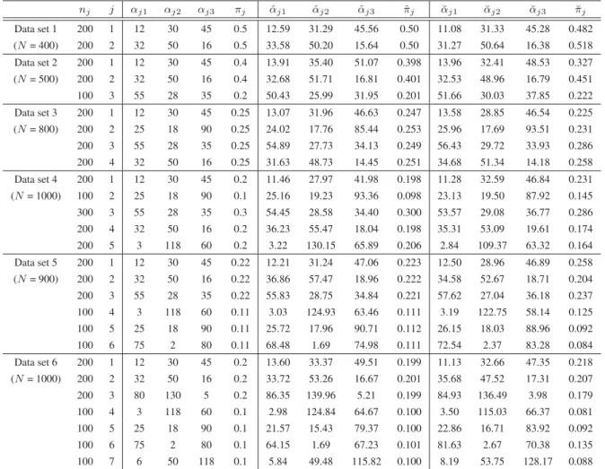
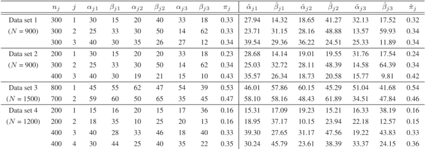
Table 2.1: Parameters of the different generated data sets.N denotes the total number of elements,

nj denotes the number of elements in clusterj. αj1,αj2, αj3 andπj are the real parameters. αˆj1,

ˆ

αj2,αˆj3 andπˆj are the estimated parameters by variational inference. α˘j1,α˘j2, α˘j3andπ˘j are the

estimated parameters using DM. We can observe that both algorithms are able to estimate unknown parameters, yet the variational algorithm always gives more accurate values.

n_j j α_j₁ α_j₂ α_j₃ π_j αˆ_j₁ αˆ_j₂ αˆ_j₃ πˆ_j α˘_j₁ α˘_j₂ α˘_j₃ π˘_j Data set 1 200 1 12 30 45 0.5 12.59 31.29 45.56 0.50 11.08 31.33 45.28 0.482 (N= 400) 200 2 32 50 16 0.5 33.58 50.20 15.64 0.50 31.27 50.64 16.38 0.518 Data set 2 200 1 12 30 45 0.4 13.91 35.40 51.07 0.398 13.96 32.41 48.53 0.327 (N= 500) 200 2 32 50 16 0.4 32.68 51.71 16.81 0.401 32.53 48.96 16.79 0.451 100 3 55 28 35 0.2 50.43 25.99 31.95 0.201 51.66 30.03 37.85 0.222 Data set 3 200 1 12 30 45 0.25 13.07 31.96 46.63 0.247 13.58 28.85 46.54 0.225 (N= 800) 200 2 25 18 90 0.25 24.02 17.76 85.44 0.253 25.96 17.69 93.51 0.231 200 3 55 28 35 0.25 54.89 27.73 34.13 0.249 56.43 29.72 33.93 0.286 200 4 32 50 16 0.25 31.63 48.73 14.45 0.251 34.68 51.34 14.18 0.258 Data set 4 200 1 12 30 45 0.2 11.46 27.97 41.98 0.198 11.28 32.59 46.84 0.231 (N= 1000) 100 2 25 18 90 0.1 25.16 19.23 93.36 0.098 23.13 19.50 87.92 0.145 300 3 55 28 35 0.3 54.45 28.58 34.40 0.300 53.57 29.08 36.77 0.286 200 4 32 50 16 0.2 36.23 55.47 18.04 0.198 35.31 53.09 19.61 0.174 200 5 3 118 60 0.2 3.22 130.15 65.89 0.206 2.84 109.37 63.32 0.164 Data set 5 200 1 12 30 45 0.22 12.21 31.24 47.06 0.223 12.50 28.96 46.89 0.258 (N= 900) 200 2 32 50 16 0.22 36.86 57.47 18.96 0.222 34.58 52.67 18.71 0.204 200 3 55 28 35 0.22 55.83 28.75 34.84 0.221 57.62 27.04 36.18 0.237 100 4 3 118 60 0.11 3.03 124.93 63.46 0.111 3.19 122.75 58.14 0.125 100 5 25 18 90 0.11 25.72 17.96 90.71 0.112 26.15 18.03 88.96 0.092 100 6 75 2 80 0.11 68.48 1.69 74.98 0.111 72.54 2.37 83.28 0.084 Data set 6 200 1 12 30 45 0.2 13.60 33.37 49.51 0.199 11.13 32.66 47.35 0.218 (N= 1000) 200 2 32 50 16 0.2 33.72 53.26 16.67 0.201 35.68 47.52 17.31 0.207 200 3 80 130 5 0.2 86.35 139.96 5.21 0.199 84.93 136.49 3.98 0.179 100 4 3 118 60 0.1 2.98 124.84 64.67 0.100 3.50 115.03 66.37 0.081 100 5 25 18 90 0.1 21.57 15.43 79.37 0.100 22.86 16.71 83.92 0.092 100 6 75 2 80 0.1 64.15 1.69 67.23 0.101 81.63 2.67 70.38 0.135 100 7 6 50 118 0.1 5.84 49.48 115.82 0.100 8.19 53.75 128.17 0.088

(31)

(a) (b) (c)

(d) (e) (f)

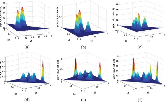
Figure 2.2: Mixture densities for the synthetic data sets. (a) Data set 1, (b) Data set 2, (c) Data set 3, (d) Data set 4, (e) Data set 5, (f) Data set 6.

2.3.1

Synthetic Data

We ﬁrst present the performance of our variational algorithm (varDM) in terms of estimation and selection, on six three-dimensional synthetic data. Please notice that, here we choose D _{= 3}

purely for ease of representation. We tested the effectiveness of our algorithm for estimating the mixture’s parameters and selecting the number of components on generated data sets with different parameters. Table 2.1 shows the real and estimated parameters of each data set using both our variational algorithm and the deterministic approach (DM) proposed in [75]. Figure 2.2 represents the resultant mixtures with different shapes (symmetric and asymmetric modes).

In order to estimate the number of components, we apply directly our algorithm on these data sets (by starting with 15 components). The redundant components have estimated mixing coef-ﬁcients close to 0 after convergence. By removing these redundant components, we obtain the correct number of components for each generated data set. Figure 2.3 illustrates the value of the

(32)

(a) (b) (c)

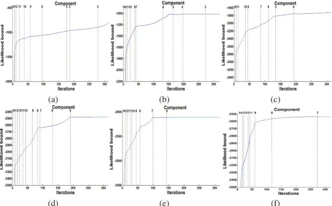
(d) (e) (f)

Figure 2.3: Variational likelihood bound for each iteration for the different generated data sets. The initial number of components is 15. Vertical dash lines indicate cancelation of components. (a) Data set 1, (b) Data set 2, (c) Data set 3, (d) Data set 4, (e) Data set 5, (f) Data set 6.

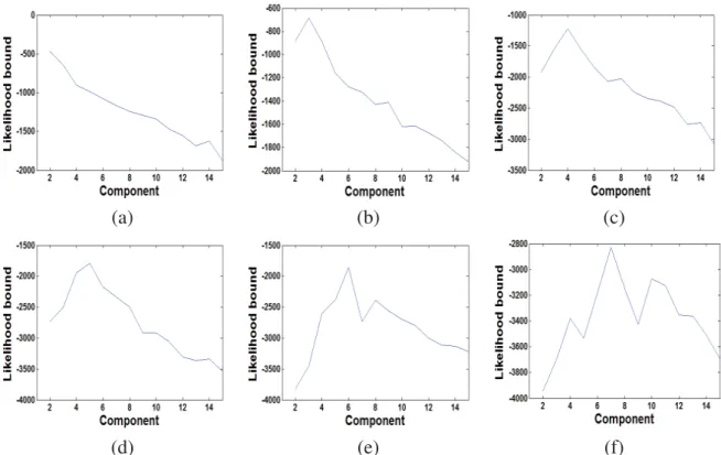
variational likelihood bound in each iteration and shows that the likelihood bound increases at each iteration and in most cases it increases very fast when one of the mixing coefficients is close to 0 (i.e. shall be removed). We can verify the results of estimating the number of components by per-forming our variational optimization on a fixed number of components (i.e. without components elimination). Thus, the variational likelihood bound becomes a model selection score. As shown in Figure 2.4, we ran our algorithm by varying the number of mixture components from 2 to 15. According to this figure, it is clear that for each data set, the variational likelihood bound is max-imum at the correct number of components which indicates that the variational likelihood bound can be used as an efficient criterion for model selection.

Moreover, we have performed a comparison between the numerical complexity of the proposed variational algorithm and the DM approach, in terms of overall computation time and number of

(33)

(a) (b) (c)

(d) (e) (f)

Figure 2.4: Variational likelihood bound as a function of the ﬁxed assumed number of mixture components for the different generated data sets. (a) Data set 1, (b) Data set 2, (c) Data set 3, (d) Data set 4, (e) Data set 5, (f) Data set 6.

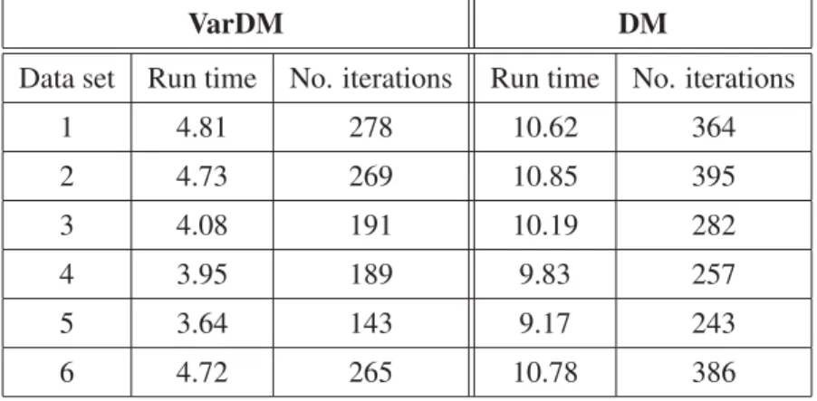
iterations before convergence. The corresponding results are shown in Table 2.2. It is obvious that, for each data set, the proposed variational algorithm requires less iterations to converge and has a faster computational time than the deterministic one.

2.3.2

Images Categorization

In this part, we consider the problem of images categorization which is a fundamental problem in vision that has recently drawn considerable interest and seen great progress [82]. Applications include the automatic understanding of images, object recognition, image databases browsing and content-based images suggestion, recommendation and retrieval [83–85]. As the majority of com-puter vision tasks, an important step for accurate images categorization is the extraction of good descriptors (i.e. discriminative and invariant at the same time) to represent these images. Recently

(34)

Table 2.2: Rum time (in seconds) and number of iterations required before convergence for varDM and DM.

VarDM DM

Data set Run time No. iterations Run time No. iterations

1 4.81 278 10.62 364 2 4.73 269 10.85 395 3 4.08 191 10.19 282 4 3.95 189 9.83 257 5 3.64 143 9.17 243 6 4.72 265 10.78 386

Table 2.3: Clustering Accuracies with varDM Model and varGM Model. M∗ denotes the average number of clusters.

varDM varGM

Data set M∗ Accuracy (%) M∗ Accuracy (%)

A 4.85±0.19 74.93±1.62 4.56±0.31 65.26±1.38 B 4.03±0.14 78.01±1.56 4.41±0.52 68.34±1.29

(35)

(a) (b) (c) (d) (e) (f) (g) (h)

Figure 2.5: Sample images from each group of sports event data set: (a) Rowing. (b) Badminton. (c) polo. (d) Bocce. (e) Snow Boarding. (f) Croquet. (g) Sailing. (h) Rock climbing.

methods based on the bag-of-features approach have shown to give excellent results [86, 87]. In this subsection we therefore follow this class of methods and in particular the one proposed in [87]. First, key points in the images are detected using one of the various detectors and local descriptors which should be invariant to image transformation, occlusions and variations of illumination are extracted. Then, these local descriptors are grouped intoWhomogenous clusters, using a cluster-ing or vector quantization algorithm such as K-Means. Therefore, each cluster center is treated as a visual word and a visual vocabulary is build with W visual words. Applying the paradigm of

bag-of-words, aW−dimensional histogram representing the frequency of each visual word is cal-culated for each image. Finally, the Probabilistic Latent Semantic Analysis (pLSA) model [88] is applied to reduce the dimensionality of the resulting histograms allowing the representation of im-ages as proportional vectors. Thus, our variational Dirichlet mixture modeling framework provides a natural setting to address the categorization task.

In our experiments, we have considered the FeiFei’s sports event data set containing 8 cate-gories of sports scenes: rowing (250 images), badminton (200 images), polo (182 images), bocce (137 images), snow boarding (190 images), croquet (236 images), sailing (190 images), and rock climbing (194 images). Thus, the data set contains 1,579 images in total. We normalize each image into a size of₂₅₆×₂₅₆pixels. Examples of images from each categories are shown in Figure 2.5.

(36)

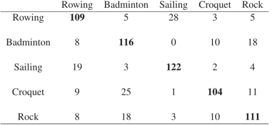
Table 2.4: Average Rounded Confusion Matrix using the varDM Model to categorize Data Set A. Rowing Badminton Sailing Croquet Rock

Rowing 109 5 28 3 5

Badminton 8 116 0 10 18

Sailing 19 3 122 2 4

Croquet 9 25 1 104 11

Rock 8 18 3 10 111

In our experiments, the key points of each image are detected using the Difference-of-Gaussian (DoG) interest point detector [89] and described using Scale-Invariant Feature Transform (SIFT) descriptor, resulting on 128-dimensional vector for each key point [89]. Then, an accelerated ver-sion of the K-Means algorithm [90] is used to cluster all the SIFT vectors into a visual vocabulary of 700 visual words. Note that, the number of visual words is user-speciﬁed. Based on our experi-ments, the best results have been obtained whenW _{= [600},_800]. Then, the new representation for each image is calculated through the pLSA model by considering 35 aspects.

Two data sets are used for testing our algorithm. Data set A consists of 750 images from ﬁve categorizes of the sports event data set: rowing, badminton, sailing, croquet and rock climbing. Data set B consists of 600 images from four different categorizes of the sports event data set: rowing, polo, snow boarding and bocce. Table 2.3 shows the average number of clusters and the average classiﬁcation accuracies using both varDM and Gaussian mixture (varGM) models learned by running their respective variational algorithms 20 times. Tables 2.4 and 2.5 show the confusion matrices when applying varDM for data sets A and B, respectively. According to the obtained results we can clearly see that the varDM outperforms the varGM in terms of both categorization accuracy and selection of the optimal number of image categories.

2.3.3

Anomaly Intrusion Detection

Nowadays, intrusion detection systems (IDSs) are becoming more and more important as com-puter security vulnerabilities and ﬂaws are being discovered everyday [91–94]. The main goal

(37)

Table 2.5: Average Rounded Confusion Matrix using the varDM Model to categorize Data Set B.

Rowing Polo Snow Bocce

Rowing 115 17 8 10

Polo 6 124 13 7

Snow 21 6 109 14

Bocce 5 3 15 127

is to establish approaches which can scan network activities and detect suspicious patterns that may have been derived from intrusion attacks. Intrusion detection is based on the assumption that intrusive activities are noticeably diverse from normal system activities and hence detectable. According to the analysis methods, IDSs can be classified into two main categories:misuse detec-tion andanomalydetection systems. In misuse detection systems, pre-defined attack patterns and signatures are used for detecting known attacks. Alternatively, anomaly detection systems detect unknown attacks by observing deviations from normal activities of the system. Anomaly detection has the advantage of detecting new types of intrusions. In our work, we first use our mixture model to learn patterns of normal and intrusive actives from training data. Then, we detect and classify intrusive activities which are deviated from the normal activities in a testing data set.

Data Set Description

The well-known KDD Cup 1999 Data 1 _{is used to investigate our mixture model. This data set}

(tcpdump file) was collected at MIT Lincoln laboratory for the 1998 DARPA intrusion detection evaluation program by simulating attacks on a typical U.S. Air Force Lan. Each data instance in the data set is a connection record obtained from the simulated intrusions with 41 features (such as duration, dst bytes, etc). A connection is a sequence of TCP packets starting and ending at some well defined times, between which data flows to and from a source IP address to a target IP address under some well defined protocol. The training data consists of 494,021 data instances of which 97,277 are normal and 396,744 are attacks. The testing set contains 311,029 data instances

(38)

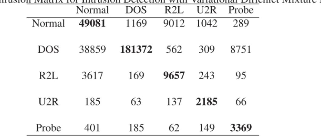
Table 2.6: Confusion Matrix for Intrusion Detection with Variational Dirichlet Mixture Model.

Normal DOS R2L U2R Probe

Normal 49081 1169 9012 1042 289

DOS 38859 181372 562 309 8751

R2L 3617 169 9657 243 95

U2R 185 63 137 2185 66

Probe 401 185 62 149 3369

Table 2.7: Intrusion Detection Results Using different approaches.

Algorithm varDM DM varGM GM

Accuracy (%) 78.75 75.53 73.34 71.29

of which 60,593 are normal and 250,436 are attacks. All of these attacks fall into one of the following four categories: DOS: denial-of-service (e.g. syn ﬂood); R2L: unauthorized access from a remote machine (e.g. guessing password); U2R: unauthorized access to local superuser (root) privileges (e.g. buffer overﬂow attack) and Probing: surveillance and other probing (e.g. port scanning).

Results

In our data set, each data instance contains 41 features in which 34 are numeric and 7 are symbolic. In our experiments, only the 34 numeric features are used (i.e. each data is then represented as a 34-dimensional vector). Since the features are on quite different scales in the data set, we need to normalize them such that one feature would not dominant the others in our algorithm. Table 2.6 shows the obtained confusion matrix using our varDM. According to this matrix the detection rate is 78.75%. A summary of the detection results by applying other approaches namely the DM, the varGM, and the Gaussian mixtures (GM) are given in table 2.7. According to these results, we can say that the varDM outperforms signiﬁcantly, according a student’s t-test, the other approaches.

(39)

Chapter 3

Unsupervised Feature Selection for

High-Dimensional Non-Gaussian Data Clustering

with Variational Inference

Clustering has been a subject of extensive research in data mining, pattern recognition and other areas for several decades. The main goal is to assign samples, which are typically non-Gaussian and expressed as points in high-dimensional feature spaces, to one of a number of clusters. It is well-known that in such high-dimensional settings, the existence of irrelevant features generally compromises modeling capabilities. In this chapter, we propose a variational inference framework for unsupervised non-Gaussian feature selection, in the context of ﬁnite generalized Dirichlet (GD) mixture-based clustering. Under the proposed principled variational framework, we simultane-ously estimate, in a closed-form, all the involved parameters and determine the complexity (i.e. both model an feature selection) of the GD mixture. Extensive simulations using synthetic data along with an analysis of human action videos demonstrate that our variational approach achieves better results than comparable techniques.

3.1

Model speciﬁcation

The GD distribution is the generalization of the Dirichlet distribution. It has a more general co-variance structure (can be positive or negative) than Dirichlet distribution and offers high ﬂexibility and ease of use for the approximation of both symmetric and asymmetric distributions. Compared to the Gaussian distribution, the GD distribution has a smaller number of parameters that makes the estimation and the selection more accurate.

(40)

A GD distribution of aD-dimensional random vectorY is deﬁned as GD(Y|αj, βj) = D l=1 Γ(αjl+βjl) Γ(αjl)Γ(βjl) Yαjl−1 l 1− l k=1 Yk γ_jl (3.1)

where D_l₌₁Yl < 1 and 0 < Yl < 1 for l = 1, . . . , D. αj = (αj1, . . . , αjD) and βj =

(βj1, . . . , βjD) are the parameters of the GD distribution, such that, αjl > 0, βjl > 0, γjl =

βjl−αjl+1−βjl+1forl = 1, . . . , D−1, andγjD =βjD−1. Assume that we have a set ofN

indepen-dent and iindepen-dentically distributed vectorsY _{= (}Y₁, . . . , YN), where each vectorYi = (Y1, . . . , YD)is

assumed to be sampled from a ﬁnite GD mixture model withM components [17]:

p₍Yi|π, α, β) = M

j=1

πjGD(Yi|αj, βj), (3.2)

whereα _{= (}α₁, . . . , αM)and β = (β1, . . . , βM). αj andβj are the parameters of the GD

distri-bution representing component j. π _{= (}π₁, . . . , πM) represents the mixing coefﬁcients with the

constraints that are positive and sum to one.

According to an interesting mathematical property of the GD thoroughly discussed in [60], the data point Yi can be transformed using a geometric transformation into another D-dimensional

data point Xi with independent features. Then, the ﬁnite GD mixture model is equivalent to the

following mixture model

p₍Xi|π, α, β) = M j=1 πj D l=1 Beta(Xil|αjl, βjl) (3.3) whereXi = (Xi1, . . . , XiD),Xi1 =Yi1andXil=Yil/(1− l−1