Learning Patterns from Sequential
and Network Data Using
Probabilistic Models
Yin Cheng Ng
A dissertation submitted in partial fulfillment of the requirements for the degree of
Doctor of Philosophy of
University College London.
Department of Statistical Science University College London
2
I, Yin Cheng Ng, confirm that the work presented in this thesis is my own. Where information has been derived from other sources, I confirm that this has been indicated in the work.
Abstract
The focus of this thesis is on developing probabilistic models for data observed over temporal and graph domains, and the corresponding variational inference algorithms. In many real-world phenomena, sequential data points that are observed closer in time often exhibit higher degrees of dependency. Similarly, data points observed over a graph domain (e.g., user interests in a social network) may exhibit higher dependencies with lower degrees of separation over the graph. Furthermore, the connectivity structures that define the graph domain can also evolve temporally (i.e., temporal networks) and exhibit dependencies over time. The data sets observed over temporal and graph domains often (but not always) violate the independent and identically distributed (i.i.d.) assumption made by many mathematical models. The works presented in this dissertation address various challenges in modelling data sets that exhibit dependencies over temporal and graph domains. In Chapter 3, I present a stochastic variational inference algorithm that enables factorial hidden Markov models for sequential data to scale up to extremely long sequences. In Chapter 4, I propose a simple but powerful Gaussian process model that captures the dependencies of data points observed on a graph domain, and demonstrate its viability in graph-based semi-supervised learning problems. In Chapter 5, I present a dynamical model for graphs that captures the temporal evolution of the connectivity structures as well as the sparse connectivity structures often observed in temporal real network data sets. Finally, I summarise the contributions of the thesis and propose several directions for future works that can build on the proposed methods in Chapter 6.
Impact Statement
The research results presented in this thesis build upon the contributions of other researchers in the machine learning and statistics communities. The completion of the works in this thesis would not have been possible without their contributions. In return, I hope that my work will benefit researchers working inside and outside of academia in the following ways.
1. As big data has become commonplace, the algorithm presented in Chapter 3 can benefit researchers who need to model big data with sequential dependency. While the algorithm was designed with a specific probabilistic model in mind, components of the algorithm can be adapted to develop scalable algorithms for other probabilistic sequential models.
2. The work should encourage researchers and practitioners to think more deeply about the dependency between data points and ways to exploit the dependency to construct better models under the probabilistic modelling framework. The result presented in Chapter 4 should serve as an example of one approach to model dependency in data sets with network structures.
3. The work presented in Chapter 5 aims to inspire researchers in social networks to develop dynamic network models that can better capture properties observed empirically in real temporal network data sets.
Acknowledgements
First of all, I would like to thank my supervisor, Ricardo Silva, for his support and generosity with his time. Our weekly meetings to discuss research ideas in the past three and a half years have truly expanded my mind and understanding of what research is all about. I would also like to thank University College London and the Department of Statistical Science for their financial support that allowed me unrestricted freedom to explore ideas in the past few years. I am grateful to Nicol`o Colombo and Sandipan Roy for the many fruitful conversations about research and beyond.
I would like to give a special shout-out to Vincent Kan for his friendship and for keeping me grounded over the years. To Colleen, for making the past three years of my life so special and memorable. Finally, I am forever in debt to my family, for their unconditional support and encouragement.
Contents
1 Introduction 13
1.1 Contributions . . . 18
2 Background 20 2.1 Probabilistic Graphical Models . . . 21
2.2 Probabilistic Time Series Models . . . 22
2.2.1 Hidden Markov Models . . . 23
2.2.2 Linear Dynamical System . . . 25
2.2.3 Switching Linear Dynamical System . . . 26
2.3 Probabilistic Network Models . . . 28
2.3.1 Mixed-membership Stochastic Blockmodels . . . 29
2.3.2 Dynamic Mixed-membership Stochastic Blockmodels . . . 30
2.3.3 Exchangeable Random Graphs and Limitations . . . 32
2.3.4 Edge Exchangeable Network Models . . . 33
2.4 Gaussian Processes . . . 34
2.5 Variational Inference . . . 37
2.5.1 Variational Expectation-Maximisation Algorithm . . . 40
2.5.2 Variational Inference for Latent Markov Models . . . 41
Contents 7
2.5.4 Challenges and Innovations in Variational Inference . . . . 45
3 Scalable Variational Inference for Factorial Hidden Markov Models 48 3.1 Factorial Hidden Markov Models . . . 50
3.2 Review: Gaussian Copulas, Stochastic Variational & Amortised Inference . . . 52
3.2.1 Gaussian Copulas . . . 52
3.2.2 Stochastic Variational Inference . . . 52
3.2.3 Amortised Inference and Recognition Neural Networks . . . 53
3.3 Message-free Stochastic Variational Inference . . . 54
3.3.1 Variational Chains of Bivariate Gaussian Copulas . . . 55
3.3.2 Feed-forward Recognition Neural Networks . . . 56
3.3.3 Learning Recognition Network and Model Parameters . . . 58
3.4 Related Work . . . 60
3.5 Experiments . . . 61
3.5.1 Algorithm Validation . . . 62
3.5.2 Scalability Verification . . . 63
3.6 Discussions . . . 67
4 Gaussian Processes for Bayesian Semi-supervised Learning on Graphs 68 4.1 Background . . . 69
4.1.1 Gaussian Processes . . . 70
4.1.2 Scalable Variational Inference for Gaussian Processes . . . 71
4.1.3 The Graph Laplacian . . . 72
4.2 Graph Gaussian Processes . . . 73
4.2.1 An Alternative View of the Graph Gaussian Processes . . . 76
Contents 8
4.2.3 Computational Complexity . . . 78
4.3 Related Work . . . 78
4.4 Experiments . . . 80
4.4.1 Semi-supervised Classification on Graphs . . . 80
4.4.2 Active Learning on Graphs . . . 82
4.5 Discussions . . . 85
5 Edge Clustering Dynamic Network Model 86 5.1 Sparse Temporal Networks . . . 87
5.1.1 Sparsity . . . 88
5.1.2 Community Structure . . . 89
5.1.3 Social Influence . . . 89
5.2 Dynamic Edge Exchangeable Network Model . . . 90
5.2.1 Edge Exchangeable Sparse Networks . . . 90
5.2.2 Community Structure Mixture Model . . . 91
5.2.3 Markov Dynamics with Social Influence . . . 92
5.2.4 Poisson Vertex Birth Mechanism . . . 94
5.2.5 Model Summary . . . 95
5.3 Variational Inference . . . 97
5.3.1 Computational Complexity . . . 98
5.4 Comparisons to Existing Models . . . 99
5.5 Related Work . . . 100
5.6 Experiments . . . 101
5.6.1 Sparse Networks Simulations . . . 102
5.6.2 Link Predictions . . . 103
Contents 9
5.7 Discussions . . . 109
6 Conclusion and Future Works 110
Appendices 114
A Variational Inference Algorithm for the Dynamic Network Models 114
List of Figures
2.1 This figure shows a directed probabilistic graphical model represen-tation of the hidden Markov model. . . 23 2.2 This figure shows some samples drawn from a 4-state HMM with
2-dimensional Gaussian emission distributions. . . 24 2.3 This figure shows a directed probabilistic graphical model of the
switching linear dynamical system. . . 27
3.1 This figure shows the simulated data set in the validation experiments together with the ground truth and the learned parameters. . . 63 3.2 This figure shows the log-likelihood results from the factorial hidden
Markov model scalability experiments, demonstrating scalability with respect to the sequence length. . . 66 3.3 This figure shows the log-likelihood (y-axis) results from the
facto-rial hidden Markov model scalability experiments, demonstrating scalability with respect to the number of hidden Markov chains. . . 66
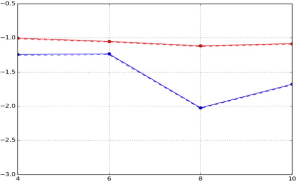
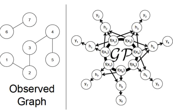
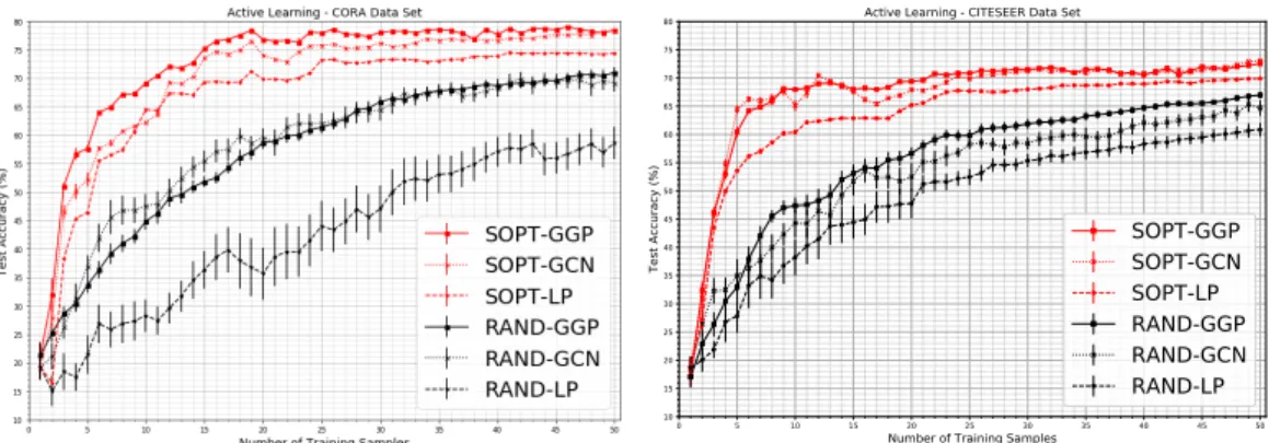
4.1 This figure shows a relational graph and the corresponding graph Gaussian process. . . 75 4.2 This figure shows the experimental results from the active learning
experiment. . . 84
5.1 The figure shows the generative process for a sequence of 3 temporal networks with 2 communities. . . 96 5.2 This figure shows some simulation results that demonstrate the
pro-posed model can indeed model sparse networks. . . 103 5.3 This figure shows the ROC curves from the link prediction experiment.106
List of Figures 11
5.4 This figure shows the experimental results from the community detection experiment. . . 108
List of Tables
3.1 This table shows the experimental results from the factorial hidden Markov model validation experiment. . . 63 3.2 This table shows the experimental results for the household power
consumption data set. . . 65
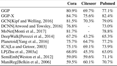
4.1 This table shows a summary of the benchmark data sets used in the semi-supervised classification experiment. . . 81 4.2 This table shows the experimental results from the semi-supervised
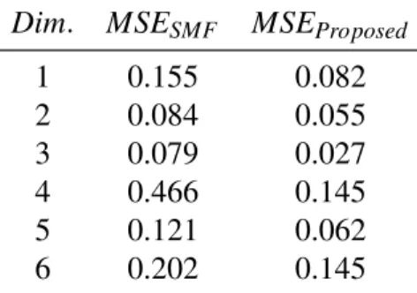
classification experiment. . . 81 4.3 This table shows the experimental results from the active learning
experiment. . . 84
5.1 This table shows the experimental results from the link prediction experiment (Challenge 1). . . 105 5.2 This table shows the experimental results from the link prediction
1
Introduction
Data sets observed in the real-world can arise from many different complex pro-cesses. Some processes include dynamical components that result in observations which exhibit sequential dependency and repeatable patterns over time. Some other processes may include interactive components where interactions between entities in the system result in observations that exhibit dependency with respect to the patterns of interactions. The interactions between entities in the system form a network, and is often expressed as a graph. For example, data points observed on entities (i.e., node labels in a network) that have interacted can exhibit dependency as a result of the interactions. Additionally, networks that encode patterns of interactions between entities can also exhibit sequential dependency as a result of underlying dynamical components that drive the system. Sequential and network dependencies are very important features of many data sets. These features should be accounted for and exploited by statistical models whenever possible in order to adequately capture the patterns in the data sets.
Examples of sequential data are abundant in our everyday lives, ranging from the music that we listen to, to the DNA sequences that encode our biological traits. Another setting where important sequential data sets are collected is in the financial markets, where participants buy and sell financial products at prices informed by in-formation available to the participants. The time series of transaction prices recorded
14
in the markets can exhibit both sequential and cross-sectional dependencies due to the varying speeds of market participants in receiving, processing and reacting to information, among many other reasons. As the technologies to capture, process and store sequential data improve, more and more sequential data sets that are extremely long and rich in structures have become available for analysis. A relevant exam-ple is the increasing adoptions of smart electricity meters which record household electricity consumption at minute intervals. The higher frequency at which the data is captured not only results in longer sequences, but also captures intra-day usage patterns which were not previously available. The availability of long sequential data sets with rich structures calls for powerful and flexible models that can scale up to the sizes of these data sets. Furthermore, sequential data sets are not restricted to vector-valued sequences. Another interesting type of sequential data sets that are often observed in the real-world are temporal sequences of network data, which I will discuss later in this section.
Apart from sequential dependency, another type of dependency that is both important and commonplace in real-world data sets is network dependency. In data sets where network structures exist, the data points are typically viewed as vertices1 in the networks and the network edges2represent the relationships between the data points. The presence of an edge between two vertices (i.e., 1-hop neighbours) typi-cally implies positive associations between the two data points on the vertices. While no theorem dictates that 1-hop neighbours are always positively associated, such positive associations are widely observed empirically, and is known as homophily in the literatures [Goldenberg et al., 2010]. The dependencies between vertices fade away as the numbers of hops between pairs of vertices increase. As such, it is natural to view the network structure as an irregular coordinate system in non-Euclidean space where distances between pairs of data points are measured in the numbers of hops separating the pairs. Looking at network data through this coordinate system view allows us to draw parallels between sequential and network dependencies, in
1Vertices are also referred to as nodes in the literatures.
15
that sequential data consists of a list of data points ordered on a regular 1-dimensional grid in the Euclidean space, and the dependencies between pairs of data points in the sequence decrease as the Euclidean distances between them increase.
Examples of network data in the wild include communication networks, where vertices and edges represent individuals and their interactions respectively; computer networks where computers are connected through communication links; rail networks where train stations are connected by train tracks, and many others. A particularly illustrative example of network data are citation networks. Vertices in citation network are academic publications, and the edges in the network connect each vertex to a list of other publications cited in its bibliography. Each vertex may also include covariates, such as the bag-of-word representation of the publication, as well as a label that indicates the field/sub-field that the publication is associated with. As academic papers that belong to the same sub-fields are more likely to cite each others, the vertex labels of neighbours are typically positively associated, giving rise to dependency over the citation network connectivity structure. Clearly, the network dependency should be taken into account when building statistical models.
In addition to data sets with naturally observed network structures, practitioners have also invented various heuristics and algorithms to create networks for inde-pendently and identically distributed (i.i.d.) data sets that can suitably represent the relationships between the data points (e.g., Argyriou et al. [2006]). The derived network representations allow powerful algorithms that operate on networks to be applied to the data sets.
Network data sets are complex in nature, with a multitude of properties that can be difficult to capture by any single model. Understanding different aspects of a network data set often requires modellers to look at the data through many different lenses. The description of networks in the previous paragraphs assumed that the fundamental datum of the network data sets is the vertex. While many existing models and algorithms implicitly make the same assumption of treating vertices as the fundamental data unit, this is by no mean the only way to think about networks.
16
Given different modelling objectives, it may be more intuitive and productive to think of edges, triplets, hyper-edges or even paths in the networks as the fundamental units, as discussed in details in Crane [2018], and model them as such.
Moving Average Models: Sequences and Networks
Moving average process is one of the most fundamental and well-known stochastic process in the time series literature. Given a sequence indexed by positive integers(y1,y2,y3, . . .), the
moving average process models the dependency between data points in a sequence as
yt= q
∑
s=1
asεt−s+εt (1.1)
whereεt∼ N(0,σ2)is a sequence of i.i.d. Gaussian white noise anda1, . . . ,aqare the model
parameters. The model in Equation (1.1) is known as theMA(q)process. The auto-covariance structure of the sequence as specified byMA(q)can be easily derived from the first principle.
The moving average model can also be extended to data sets with network structure. Given data points{yn|n∈1, . . . ,N}observed on the vertices of a networkGwithNvertices, one can
specify yn= q
∑
s=1 as |Ne(s,n)|∑
i∈Ne(s,n) εi +εn (1.2)whereεn∼ N(0,σ2),a1, . . . ,aqare model parameters andNe(s,n)is the set of indices denoting
thes−hop neighbours of vertexn. For q=1, it is easy to see that
y∼ N(0,PP|) (1.3) wherey= [y1, . . . ,yN]T,P= (I+D)−1(I+A),A∈ {0,1}N×Nis the adjacency matrix for the
networkGandD∈ZN×Nis the diagonal vertex degree matrix.
The models specified in Equation (1.1) and (1.2) are similar in that the data points are dependent on their adjacent data points. However, the notions of adjacency differ in the two scenarios. In the sequential data, adjacent data points are defined as the data points that precede the data point of interest. In the network, adjacent data points refer to the neighbours of the data point of interest at different hops. The two models presented above illustrated the conceptual similarities between modelling sequential and network data sets.
17
In addition to the data points observed on the vertices of network, the connec-tivity structure of the network itself is often of modelling interest. While the network connectivity often exhibits rich structure, it is difficult to gain deeper insights, such as understanding the community structure of the network, without models. Net-work data sets are intrinsically temporal as it is extremely rare to observe all the vertices and edges of a network at the same moment in time: vertices typically join the network at different time points while connections form and vanish over time. Therefore, it may be important to account for the temporal aspect of network data sets using dynamic network models whenever possible.
One example of the network data sets in which the temporal aspect is important is the communication network. In a communication network, users of the communi-cation service (e.g., e-mails, telecommunicommuni-cations etc.) are represented by the vertices, and the communication records between pairs of users are the edges. The edges are typically time-stamped at the moment when the users communicate. Aggregating the edges that are observed daily, we can construct a sequence of communication networks in which each network in the sequence represents a snapshot of com-munications between the users during the day. The sequence of networks may be temporally correlated as users who had communicated previously are more likely to communicate again in the near-future.
The focus of this thesis is on the development of probabilistic models and variational inference algorithms that can capture the non-trivial dependency struc-tures of sequences, networks and sequences of networks data sets. The probabilistic models of primary interest are probabilistic graphical models (PGMs) and Gaussian processes (GPs). These probabilistic methods provide a convenient, modular and powerful way to specify models that can capture different types of dependency struc-ture intended by the modellers. However, performing Bayesian inference in complex probabilistic models has remained a difficult challenge without a satisfying universal solution, and requires bespoke approximate inference algorithms to be developed. Therefore, in addition to proposing novel probabilistic models for dependent data,
1.1. Contributions 18
the development of suitable variational inference algorithms for the proposed mod-els forms a key part of this thesis. A review of the core concepts, algorithms and probabilistic models that are the building blocks of the works presented in this thesis is available in Chapter 2.
1.1
Contributions
The contributions made in this dissertation are summarised as follow:
1. The proposal of a novel scalable variational inference algorithm for factorial hidden Markov models (FHMMs) in Chapter 3. The proposed algorithm extends the stochastic variational inference algorithm proposed in Hoffman et al. [2013] to FHMM, and takes advantage of a novel Gaussian-Bernoulli copula parameterization of Markov chain variational distribution that lends itself to amortized inference using feed-forward recognition neural networks. The computational complexity of the proposed algorithm is sub-linear with respect to the length of the data sequences, allowing FHMMs to be applied to very long sequences under limited computing budgets. This is a joint work with Pawel Chilinski.
2. The proposal of a data efficient Gaussian process model for semi-supervised learning on graphs in Chapter 4. The proposed model shows extremely compet-itive performance when compared to the state-of-the-art graph neural networks on semi-supervised learning benchmark experiments, and outperforms the neural networks in active learning experiments where labels are scarce. Fur-thermore, the model does not require a validation data set for early stopping to control over-fitting. The model can be viewed as an instance of empirical distribution regression weighted locally by network connectivity. Its intuitive construction is further motivated by a Bayesian linear model interpretation where the node features are filtered by an operator related to the graph Lapla-cian. The method can be easily implemented by adapting off-the-shelf scalable
1.1. Contributions 19
variational inference algorithms for Gaussian processes.
3. The proposal of a dynamic edge exchangeable random network model that can capture sparse connections observed in real temporal networks, in contrast to existing dynamic models which can only model dense networks. The model achieved good link prediction accuracy on multiple data sets when compared to the benchmark models, and is able to extract interpretable time-varying community structures from the data. In addition to sparsity, the model accounts for the effect of social influence on vertices’ future behaviours. Compared to the dynamic blockmodels, the proposed model has a smaller latent space. The compact latent space requires a smaller number of parameters to be estimated in variational inference and results in a computationally friendly inference algorithm.
The works presented in Chapter 3 and Chapter 4 have been published as the following self-contained articles in conference proceedings.
• Y.C. Ng, P. Chilinski, R. Silva. Scaling Factorial Hidden Markov Models: Stochastic Variational Inference without Messages. In NIPS, 2016.
• Y.C. Ng, N. Colombo, R. Silva. Bayesian Semi-supervised Learning with Graph Gaussian Processes. To appear in NIPS, 2018.
2
Background
In this chapter, I survey important concepts, models and algorithms that are the building blocks of the works presented in this dissertation, and provide relevant references to the literatures. The topics surveyed in this chapter are general and non-exhaustive. Technical concepts that are more specific to the three pieces of work presented in this dissertation are surveyed in the relevant chapters.
At the core of probabilistic models are joint probability distributions that specify the statistical dependencies between the observed data and a set of latent random vari-ables that explain the data. In Section 2.1, I survey the probabilistic graphical model (PGM) as a flexible framework to compose joint probability distributions over a large number of random variables, with a focus on the directed PGMs. In Section 2.2, I introduce the dynamic directed graphical models, which are discrete-time stochastic processes constructed through recursively specified conditional distributions. The two types of dynamic PGM discussed are the hidden Markov Model (HMM) and the linear dynamical system (LDS). The HMM is relevant to the work presented in Chapter 3 while the LDS is related to the work in Chapter 5.
In Section 2.3, I discuss some graphical models for network data sets. The probabilistic graphical models for networks are related to the models proposed in Chapter 5. Starting with some discussions on the probabilistic graphical models for
2.1. Probabilistic Graphical Models 21
static network, I then proceed to discuss their dynamic extensions through temporally coupling the graphical models for static network using LDS and HMM. The resulted dynamic network models can capture the temporal evolution of the connectivity in sequences of networks.
In addition to the probabilistic graphical models, I discuss the Gaussian process (GP) as a flexible Bayesian non-parametric model for supervised learning in Sec-tion 2.4. Using the vanilla GP as a building block, I propose a simple but effective Bayesian model for semi-supervised learning on graphs in Chapter 4.
Finally, I discuss the variational inference algorithms in Section 2.5. Variational inference serves as an important tool to approximate the intractable posterior distri-butions encountered in probabilistic models, and is extensively used in the works presented in the dissertation.
2.1
Probabilistic Graphical Models
A rich framework to construct high-dimensional joint probability distribution of data is the probabilistic graphical model (PGM). PGM allows a joint distribution to be decomposed into a product of factors. The decomposition allows for a more succinct representation of the probabilistic model compared to a direct specification of the joint distribution because of the inductive bias introduced in the decomposition process. Additionally, inference for PGMs can be performed using a suite of well-developed algorithms.
The two main categories of PGMs are the directed graphical models and the undirected graphical models. Directed graphical models are typically chosen when there is plausible hierarchical or causal structure in the data, such that the joint distributions can be factorised accordingly. The time series and network models of interest in this report mainly fall into the directed graphical model category because of the causal nature of time and the hierarchical structure in network interactions [Fox, 2009].
2.2. Probabilistic Time Series Models 22
More formally, a directed graphical model is a directed acyclic graph (DAG) where each node in the DAG represents a random variable with directed incoming edges from its parent nodes and outgoing edges to its child nodes. The joint proba-bility distribution for the random variables of interest can be expressed as a product of conditional distributions, with one conditional distribution for each node in the DAG and a conditioning set that corresponds to its parent nodes. Two nodes in the DAG that are independent a priori may be conditionally dependent when conditioned on their common descendants. This phenomenon is known as explaining away, and plays a critical role in determining the conditional independence relationships encoded by the directed graphical model. To efficiently determine the conditional independence relationships encoded by a directed graphical model, one can make use of the Bayes ball algorithm [Murphy, 2012].
Inference in PGMs amounts to computing the conditional probability distribu-tions of the unobserved random variables conditioning on the observed data, known as the posterior distributions. For tree-structured PGMs, inference can be performed efficiently using dynamic programming algorithms that exploit the conditional in-dependence structure of the graphical models [Barber, 2012]. However, computing the posterior distributions of general PGMs are typically difficult because of the in-tractable high-dimensional integrals and/or summations in the normalising constants that need to be evaluated. Therefore, practitioners resort to approximate inference algorithms to approximate the posterior distributions.
2.2
Probabilistic Time Series Models
In this section, I briefly review the hidden Markov model (HMM), the linear dy-namical system (LDS) and the switching linear dydy-namical system (sLDS). These probabilistic time series models are stochastic processes that can be expressed as dynamic directed graphical models.
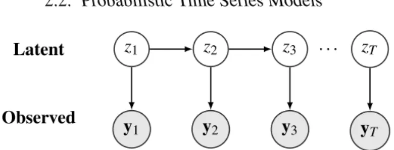
2.2. Probabilistic Time Series Models 23
Latent z1 z2 z3 zT
Observed y
1 y2 y3 yT
. . .
Figure 2.1:This figure shows a directed probabilistic graphical model of the hidden Markov
model. This is also a valid graphical model for the linear dynamical system when the latent variables are continuous. The structure of the graphical model implies that conditioning on
the present latent variablezt0, the latent variables in the futurezt>t0 are independent of the
latent variables in the pastzt<t0.
sub-sections, we describe a powerful extension of the HMM called the factorial HMM in chapter 3, and propose a scalable variational inference algorithm for the factorial HMM. In chapter 5, we propose a dynamic network model that leverages a variant of the LDS to model the temporal dependence in dynamic networks.
2.2.1
Hidden Markov Models
The hidden Markov model is a class of discrete time stochastic process with a latent discrete-valued Markov process where given the latent state at a particular time point, the observation is independent of other observations and distributed according to the state-specific probability distributions. The probability distributions for observations (i.e., the emission distributions), can either be discrete or continuous depending on the type of data observed. Intuitively, HMMs can be thought of as mixture models where the data point specific latent cluster assignments are distributed according to the underlying Markov process.
Given a sequence of observationsy1, ...,yT, the joint probability distribution of the observed sequence and the corresponding latent states of the Markov process
z1, ...,zT parameterised by the model parametersθ are as follow.
pθ(y1:T,z1:T) =pθ(z1)pθ(y1|z1)
T−1
∏
t=2
pθ(zt|zt−1)pθ(yt|zt) (2.1)
2.2. Probabilistic Time Series Models 24
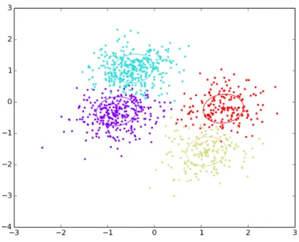
Figure 2.2:This figure shows some samples drawn from a 4-state HMM with 2-dimensional
Gaussian emission distributions. The stars represent the means of the Gaussian distributions and the ellipses represent the covariance. The colored dots are the samples. The colors encode the 4 different states of the HMM.
pθ(z1), thetransition distribution pθ(zt|zt−1)and theemission distribution pθ(yt|zt). The initial and transition distributions of the Markov process are typically chosen to be categorical distributions. The model parametersθ can be estimated from the data
using the expectation-maximisation (EM) algorithm [Dempster et al., 1977]. Given the observed sequencey1:T, exact inference in HMM can be performed efficiently with dynamic programming algorithms as the corresponding graphical model has tree structure that implies conditional independence between the future and the past given the current latent state. The inference tasks of interest are filtering, smoothing and forecasting, which correspond to computing p(zτ|y1:τ), p(zτ|y1:T) and p(zT+n|y1:T)respectively where τ∈ {1, ...,T−1}and n∈Z+. The standard Forward-Backward algorithm to compute these distributions are detailed in standard machine learning textbooks such as [Murphy, 2012].
2.2. Probabilistic Time Series Models 25
2.2.2
Linear Dynamical System
The linear dynamical systems are probabilistic time series models with a latent Gaussian Markov chain and observation probability distributions that are condition-ally independent given the latent states at the corresponding time points. A LDS is essentially equivalent to a HMM with continuous latent states. Therefore, the LDS shares the same graphical model representation and conditional independence relationships as the HMM.
Given a sequence of observationsy1, ...,yT, the joint probability distribution of the observed sequence and the corresponding real-valued multivariate state vectors h1, ...,hT with the model parametersθ are as follow.
pθ(y1:T,h1:T) =pθ(h1)pθ(y1|h1)
T−1
∏
t=2
pθ(ht|ht−1)pθ(yt|ht) (2.2)
In contrast to the HMM, the initial distribution pθ(h1)and transition distribu-tionpθ(ht|ht−1)are chosen to be multivariate Gaussian distributionsN(µI,ΣI)and N(Aht−1,ΣQ)respectively. The emission distribution pθ(yt|ht)is typically a multi-variate Gaussian distributionN(Cht,ΣR), but can be chosen to suit the sequences of modelling interest.
Inference in LDS is highly similar to inference in HMMs. The filtering, smooth-ing and predictive distributions, p(hτ|y1:τ), p(hτ|y1:T) and p(hT+n|y1:T), can be computed using the same forward-backward algorithm, with the summations over the latent states replaced with integrals that can be solved analytically because of the model’s linear Gaussian structure.
While the linear Gaussian structure of the model allows for tractable inference, it also imposes restrictions on the model’s flexibility. Johnson et al. [2016] improved the flexibility of LDS at the expense of tractability by replacing the linear emission distribution meanCht with a flexible black-box function fθ(ht)and developed a tractable variational inference algorithm to approximate the posterior distributions.
2.2. Probabilistic Time Series Models 26
Recent innovations in deep learning combined with advances in approximate in-ference techniques have opened up interesting opportunities to extend LDS for challenging modelling tasks.
2.2.3
Switching Linear Dynamical System
The switching linear dynamical system (sLDS) is an extension of LDS to allow the parameters of the transition and emission distributions at each time step to be chosen from a dictionary of parameters, each of which may fit particular segments of the time series data better than the other parameters. Therefore, sLDS have been applied to model complex time series that exhibit different properties over different segments [Barber et al., 2011].
To select a suitable set of parameters from the dictionary for each time step, a new discrete latent statest at each time step is introduced to the model such that the transition and emission distributions are conditional onst. The dynamics for the sequence of latent statess1, ...,sT are typically modelled with a Markov process, but can be further adapted to modelling requirements [Linderman et al., 2016].
Expanding the LDS parameter notationsθ ={µI,ΣI,A,ΣQ,C,ΣR}to sLDS withK parameter states (i.e., st ∈ {1, ...,K}), the model parameters for the sLDS areθ={{µI(1), ...,µI(K)},{Σ(I1), ...,Σ(IK)},{A(1), ...,A(K)},{ΣQ(1), ...,Σ(QK)},{C(1), ...,
C(K)},{ΣR(1), ...,Σ(RK)}}. Givenst, the transition and emission distributions are there-fore N(A(st)h t−1,Σ (st) Q ) and N(C (st)h t,Σ (st)
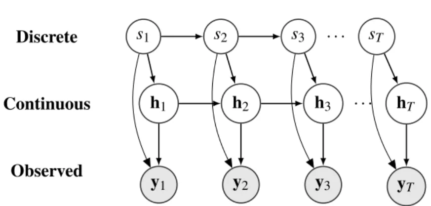
R ) respectively. The joint probability distribution of sLDS with a Markov process distributed parameter state-space is as follow pθ(y1:T,h1:T,s1:T) =pθ(h1|s1)pθ(y1|h1,s1)pθ(s1) T−1
∏
t=2 pθ(yt|ht,st)pθ(ht|ht−1,st)pθ(st|st−1). (2.3)2.2. Probabilistic Time Series Models 27 Discrete s1 s2 s3 sT Continuous h1 h2 h3 hT Observed y1 y2 y3 yT . . . . . .
Figure 2.3: This figure shows a directed probabilistic graphical model of the switching
linear dynamical system.
as the exact filtering distributions, which are mixtures of Gaussians, have numbers of components that increase exponentially with respect to their time indices. For example, the filtering distribution p(ht|y1:t,st)for a sLDS withK components is a mixture ofKt−1 Gaussians. The difficulty to keep track of the Gaussian mixtures demands inference algorithms that can sufficiently approximate the multi-modal posterior distributions without incurring exponential memory cost. Some pointers to tractable inference algorithm for sLDS can be found in [Barber et al., 2011, Murphy, 2012].
2.3. Probabilistic Network Models 28
2.3
Probabilistic Network Models
Network data are data sets that express the relationships between multiple entities that are known as vertices or nodes. A network G consists of a set ofN vertices V, typically indexed by positive integers up to N (i.e.,V ={1, ...,N}), and a set of 2−tuplesE that specifies the relationships between the vertices in V (e.g.,E =
{(1,3),(2,3),(1,2)}). In directed networks, the order of the vertices in tuple encodes the origin/destination relationship between two vertices, such that(i,j)implies a directed edge from vertexito vertex j. In undirected networks, the ordering is simply ignored. A network can also be equivalently expressed using aN×Nbinary-valued adjacency matrixY, withYi j =1 if(i,j)∈ E and 0 otherwise. The binary-valued matrix is also known as a graph, and in the case when its elements are random variables, it is called a random graph. Many probabilistic network models essentially define probability distributions on random graphs.
In this section, we briefly review some probabilistic network models and con-cepts that are relevant to the edge-exchangeable dynamic network models described in Chapter 5. We first describe the mixed-membership stochastic blockmodel and its dynamic network variant. Using the intuition developed, we then briefly describe exchangeable random graphs, in which mixed-membership stochastic blockmodel and many other probabilistic network models are special cases, and discuss their inherent limitations in modelling real-world network data. The discussions serve as a foundation for the dynamic network model that we propose in chapter 5. Finally, we review the concept of edge-exchangeability in network modelling. The model proposed in chapter 5 falls under the edge-exchangeable framework.
We refer readers who are interested in an in-depth survey of probabilistic network models to Goldenberg et al. [2010]. The excellent survey paper covers an extensive list of probabilistic network models and properties of networks that are commonly observed in the real-world.
2.3. Probabilistic Network Models 29
2.3.1
Mixed-membership Stochastic Blockmodels
A common approach to model network data is to assume that the vertices in the data set can be categorised into several clusters, and the probability of interaction between two vertices is dependent on their unobserved cluster assignments. As the cluster assignments of the members are unobserved, they are assumed to be latent variables that can be inferred from the network data. This data generative process is known as stochastic blockmodel (SBM), first proposed by Nowicki and Snijders [2001].
Mixed-membership stochastic blockmodel (MMSB) [Airoldi et al., 2008] gen-eralises the SBM to allow vertices to take on different cluster assignments depending on the vertices they are interacting with. Therefore, the cluster assignments of the vertices are unique to the vertices they are interacting with, and are sampled from from vertex-specific multinomial distributions. For example, in a directed network with 3 clusters, vertex A may belong to cluster 1 in a directed interaction from vertex A to B, and belong to cluster 2 in an interaction from A to C while belonging to cluster 3 in an interaction from B to A. Given the cluster assignments of two interacting vertices, the probability of forming a connection between the two vertices is the corresponding probability between the two clusters.
To sample a directed networkGwithNvertices and adjacency matrixYfrom a MMSB withK clusters, one can draw samples using the generative process in Algorithm 1. The algorithm was first presented in Airoldi et al. [2008]. Modification of the procedure to sample undirected network requires only trivial changes to enforce symmetry to the cluster indicators.
The MMSB requires 3 hyper-parameters to be specified. These hyper-parameters are the number of verticesN∈Z+, the concentration hyper-parameter
α ∈RK+ for the Dirichlet prior distribution of the mixed-membership vector and the
B∈[0,1]K×K matrix that describes the probabilities of connections between differ-ent mixed-membership clusters. The generative process implies a joint probability distribution as specified in Equation (2.4), which consists ofN2+N latent variables. In Equation 2.4,Ypq∈ {0,1} is an entry in the adjancency matrix that describes
2.3. Probabilistic Network Models 30
Algorithm 1Data generating process for the MMSB. Input: N∈Z+,α∈RK+,B∈[0,1]K×K
Output: Adjacency matrixY∈0,1N×N 1: for p←1 to N do
2: Sample a mixed-membership vector: πp∼Dirichlet(α)
3: for p←1 to N do 4: forq←1 to N do
5: Sample a 1-hot column vector: zp→q∼Categorical(πp)
6: Sample a 1-hot column vector: zp←q∼Categorical(πq)
7: Sample an edge: Ypq∼Bernoulli(zTp→qBzp←q)
the network data, zp→qand zp←q are indicator random variables that indicate the community memberships of vertex pandqrespectively as they interact with each other. These community assignment random variables are assumed to be sampled from vertex-specific categorical distributions parameterised byπp.
p(Y,Z→,Z←,π1:N) = h
∏
p,q p(Ypq|zp→q,zp←q,B)p(zp→q|πp)p(zp←q|πq) ih∏
p p(πp|α) i (2.4)Exact posterior inference in MMSB is intractable because of the large number of latent variables that need to be marginalised. As a result, many approximate inference and sampling algorithms, such as the algorithms proposed in Airoldi et al. [2008], Gopalan et al. [2012] and Chang [2011], have been developed.
Despite its popularity in the statistical network modelling community, MMSBs are not able to capture the sparsity of edges commonly observed in real network data. We discuss the limitation in more details in Section 2.3.3.
2.3.2
Dynamic Mixed-membership Stochastic Blockmodels
Networks that are observed in real-life often evolve over time, with new edges and vertices entering the networks at different time points while some existing edges disappear. Modelling these time-evolving networks can often reveal interesting time-varying patterns of the networks, and even allows us to make predictions. Many different probabilistic dynamic network models have been proposed by different authors [Ho et al., 2011, Xu and Hero, 2014, Heaukulani and Ghahramani, 2013,
2.3. Probabilistic Network Models 31
Algorithm 2Data generating process for the dM3SB .
Input: C,N,T ∈Z+,v∈RK×1,Φ∈RK×K,Σ1:C∈RK×K,δ ∈∆K,B∈[0,1]K×K
Output: A sequence of adjacency matrices[Y(1), ...,Y(T)], whereY(t)∈ {0,1}N×N 1: forh←1 to Cdo .Sample a sequence of latent states 2: Sampleµh(1)∼ N(v,Φ)
3: fort←2 to T do
4: Sampleµh(t)∼ N(µh(t−1),Φ)
5: fort←1 to T do 6: for p←1 to N do
7: Samplec(pt)∼Categorical(δ).Sample mixture component indicator
8: Sampleγ(pt)∼ N(µ(t)
c(pt) ,Σ
c(pt)
) .Sample mixed-membership vector 9: Transformπp(t)←So f tmax(γ(pt))
10: for p←1 to N do .Sample a network as in Algorithm 1 11: forq←1 to Ndo 12: Samplez(pt→) q∼Categorical(π (t) p ) 13: Samplez(pt←) q∼Categorical(πq(t)) 14: SampleY(pqt)∼Bernoulli(z (t) p→q T Bz(pt←) q)
Sarkar and Moore, 2006, Sewell et al., 2017, Durante and Dunson, 2014].
The review in this section focuses on the dynamic mixture of mixed-membership stochastic blockmodel (dM3SB ) proposed by Ho et al. [2011]. dM3SB extends the MMSB in two directions. Firstly, dM3SB replaces the Dirichlet prior of the mixed-membership vector with a mixture of logistic normal prior, such that the mixture model can capture both the covariance between different clusters and the multi-modal data densities. Secondly, dM3SB models the time dependency of the networks by chaining the mixture of logistic normal priors at adjacent time points with a Gaussian random walk state-space.
The generative process to sample a time series ofT networksG1, ...,GT with adjacency matricesY(1), ...,Y(T)among a set ofNverticesV from a dM3SB withK
mixed-membership clusters andCstate-space mixture components is as described in Algorithm 2.
computation-2.3. Probabilistic Network Models 32
ally intractable. A structured mean-field variational inference and a variational EM algorithms were developed to allow tractable posterior inference and learning by Ho et al. [2011].
2.3.3
Exchangeable Random Graphs and Limitations
A networkG= (V,E)with an adjacency matrixYis invariant to the relabelling of the verticesV. Roughly speaking, this means that renaming the vertices inG does not alter the information contained in the data. The invariant property, defined in Definition 2.3.1, also implies that simultaneously permuting the rows and columns ofYhas no effect on the network represented byY. A random graph that is jointly exchangeable is called an exchangeable random graph.
Definition 2.3.1. A random graph (Yi j) is called jointly exchangeable if (Yi j) d
= (Yπ(i)π(j))for every permutationπofZ.
The jointly exchangeable property ofYis widely exploited to define probabilis-tic network models, including the MMSB [Lloyd et al., 2012]. It is easy to see that the relabelling of vertices has no effect on the MMSB joint probability distribution in Equation (2.4). Probabilistic models for jointly exchangeable random graph are characterised and unified by the following Aldous-Hoover representation theorem [Aldous, 1981, Hoover, 1979].
Theorem 2.3.1. A random graph(Yi j)is jointly exchangeable if and only if it can be represented as follows: There is a random function F :[0,1]3→Y such that
(Yi j)= (d F(Ui,Uj,Ui,j)), where(Ui)i∈Zand(Ui,j)i,j∈Zare, respectively, a sequence
and an array of i.i.d. U ni f orm[0,1]random variables, which are independent of F.
While the theorem above assumes that (Ui)i∈Z and (U{i,j})i,j∈Z are i.i.d.
U ni f orm0,1 distributed, the uniformly distributed assumption is not a neces-sary condition given the following conditions hold as detailed in Orbanz and Roy [2015].
2.3. Probabilistic Network Models 33
1. Both(Ui)i∈Zand(U{i,j})i,j∈Zare i.i.d.
2. The random variables are independent of the random functionF. 3. The distributions of(Ui)i∈Zand(U{i,j})i,j∈Z are non-atomic.
In the case where the random graph is symmetric (undirected network), the Aldous-Hoover theorem can be expressed as a symmetric graphon function
W :[0,1]2→[0,1] [Lov´asz, 2012], such thatF(Ui,Uj,Ui,j)=d 1(Ui,j <W(Ui,Uj). A random graphGN withN vertices sampled from an exchangeable random graph model has an expected proportion of edgesp= 12R
[0,1]2W(x,y)dxdy. The expected
number of edges in the sampled undirected graph is N(N2−1)p=Θ(N2) if p>0. Therefore, networks sampled from exchangeable random graph models are guaran-teed to be either trivially empty (p=0) or dense (p>0,|E|=Θ(N2)). However, networks observed in the real-world are generally sparse (i.e.,|E|=o(N2)) [Gold-enberg et al., 2010]. Therefore, probabilistic network models and their dynamic variants that are built upon the exchangeable random graph assumption cannot fit sparse real network data well.
2.3.4
Edge Exchangeable Network Models
Definition 2.3.2. Consider the random network sequence(Gn)n, whereGnhas a set
of edgesEnthat are indexed by integers andVnare the active vertices ofEn(i.e.,Vn
is the union of all vertices inEn). (Gn)nis (infinitely)edge exchangeableif for every
n∈Zand every permutationπ of the edge indices inEn,Gn d
=G˜n, whereG˜nis the
resulted network from the permutation.
The limitation of the exchangeable random graph approach in modelling sparse network data has called for a different framework to model sparse networks. To address the issue, Crane and Dempsey [2016], Cai et al. [2016] separately proposed to model sparse networks as edge exchangeable random networks, and showed that the edge exchangeable models do indeed produce sparse networks. The notion of
2.4. Gaussian Processes 34
edge exchangeability is fundamentally different from the previously described joint exchangeability of random graphs and the Kallenberg exchangeability explored in Caron and Fox [2014]. We refer to the previously described joint exchangeability as vertex exchangeability to avoid confusion.
The vertex exchangeable random graphs, as defined in Definition 2.3.1, im-plicitly assumes that vertices are the statistical units of network data [Crane and Dempsey, 2016]. The assumption implies that as vertices are sampled or observed, the connectivity information between the set of sampled vertices (i.e., the edges and the lack of edges) become fully available. This is consistent with the approach of modelling networks as binary-valued adjacency matrices. However, many networks observed in the real world are only partial observations of the interactions. It is difficult to differentiate between non-interactions and unobserved interactions.
In contrast, the edge exchangeable models assume that edges are the statistical units of networks, and that the observed edges in networks are finite samples of an interaction process. With the edge exchangeable assumption, the models are invariant to the ordering of the edges. Therefore, the edges are drawn iid conditioning on an underlying distribution. Edge exchangeable networks are formally defined in Cai et al. [2016] in Definition 2.3.1. An in-depth discussion of the edge exchangeable models is presented in Janson [2017].
2.4
Gaussian Processes
In this section, I briefly review the powerful Gaussian process model. Gaussian process is a powerful tool in the probabilistic modelling tool kits. In chapter 4, we propose an extension of Gaussian process to model data points observed on the vertices of graphs.
Gaussian processes are a flexible class of stochastic processes that leverage the convenient properties of multivariate Gaussian distribution to specify prior probabil-ity distributions over functions f :X →Rindexed byx∈ X. The marginalisation
2.4. Gaussian Processes 35
property of the multivariate Gaussian distribution implies that the marginal distribu-tion for any finite subset of random variables from a collecdistribu-tion of jointly multivariate Gaussian distributed random variables is also a multivariate Gaussian distribution, with the mean vector and the covariance matrix specified by the corresponding sub-sets of the original joint distribution parameters. In Gaussian process, the distribution over an infinite collection of Gaussian distributed random variables f(·) is fully specified by its mean functionµ:X →Rand the positive semi-definite covariance
kernel functionkθ :X × X →Rparameterized by a small set of hyper-parameters
θ. Therefore, a GP distributed random function can be denoted as
f(·)∼ GP(µ(·),kθ(·,·)). (2.5)
In the simplest case of Gaussian process interpolation, a prior over the inter-polating function f can be specified using a GP. Once a set of observations drawn from the underlying functionDI ={(x1,f(x1)), . . . ,(xN,f(xN))}is observed, the predictive distribution at arbitrary pointxcan be analytically computed as follow
p(f(x)|DI}=
p(f(x),DI)
p(DI)
. (2.6)
The distributions p(f(x),DI)and p(DI)are multivariate Gaussian distributions with the mean vectors and the covariance matrices specified by evaluatingµ(·)andkθ(·,·) at the corresponding index sets.
The applications of GPs to model real-world data sets usually require the speci-fication of per data point likelihood functions that are coupled via a GP prior for the likelihood parameters. One typical modelling scenario that requires the specification of likelihood functions is Gaussian process regression. Given continuous valued data points with additive noise DR ={(x1,y1), . . . ,(xN,yN)}, a likelihood model
p(yn|f(xn)), where f(xn)is the ‘location’ parameter of the distribution, can be speci-fied for the data points to account for additive noise. Combining the likelihood model with a GP prior on f(x), one can compute the posterior process of f(x), p(f(x)|DR),
2.4. Gaussian Processes 36
and draw inference on the underlying function that generated the data set using the Bayes rule p(f(x)|DR}= p(f(x))∏ N n=1p(yn|f(xn)) p(DR) . (2.7)
The most commonly used likelihood function for the GP regression model is the Gaussian distribution, which conveniently allows Equation (2.7) to be computed analytically. Other than the Gaussian distribution, likelihood functions that are suitable for regression tasks include the Laplace distributions and the Student-t distributions. However, the use of non-Gaussian likelihood functions results in intractable model that requires approximate inference algorithms to compute the posterior process.
Beyond regression, Gaussian processes are also powerful priors for building classification models and latent variable models [Rasmussen and Williams, 2006, Lawrence, 2004, Byron et al., 2009]. However, performing inference in these more complicated GP models is analytically intractable and requires suitable approximate inference algorithms. Another major drawback of the GP models is the computa-tional complexity. Performing inference in GP models incurs a memory cost that scalesO(N2)and a computational cost that scalesO(N3), whereN is the number of data points in the training data setD, rendering the models to be computation-ally intractable in modelling big data sets. Fortunately, research breakthroughs in variational inference algorithms in recent years have provided feasible solutions that address both the analytically and computationally intractable aspects of Gaussian processes. I review the variational inference algorithms for GPs in Section 2.5.3.
The choice of the covariance functionkθ(x,x0), also known as the kernel func-tion, is particularly important for Gaussian processes. The covariance function deter-mines the prior covariances between pairs of random variables indexed by different values ofx, and therefore the prior probability density assigned to functions of dif-ferent smoothness and trends. For example, the commonly used squared exponential (SE) covariance functionkθ(x,x0) =σ2e−
(x−x0)T(x−x0)
2l2 assumes that prior covariance
2.5. Variational Inference 37
distance between their indices, with the rate of decay determined by the lengthscale parameterl. Therefore, SE covariance function with larger lengthscale parameter results in a GP that places higher density on smoother functions compared to another SE covariance GP with a smaller lengthscale parameter. In addition to smoothness, the covariance function can also be designed to incorporate other prior knowledge such as seasonal and linear trends. GPs with carefully designed kernels to capture specific known trends in the data are able to extrapolate sensibly, resulting in greater performances when compared to the other generic models. However, designing suitable kernel functions requires extensive expert knowledge, and the development of algorithms for automatic discovery of kernels remains an active research area [Duvenaud, 2014, Wilson, 2014].
Inputs to the kernel functions are not restricted to vector valued data only. Kernels for structured objects such as sequences, graphs and probability distributions have also been proposed, extending the scopes of kernel machines, including the Gaussian processes, to beyond vector valued data. In Chapter 4, I discuss a GP model with kernel function which operates on vertices in graphs that can also be viewed as a GP that operates on probability distributions.
As the kernel functions are critical components of Gaussian processes, I refer the readers to comprehensive reviews of different kernel functions in Duvenaud [2014] and Rasmussen and Williams [2006]. Discussions and reviews on the technical details of the Gaussian processes are available in Rasmussen and Williams [2006].
2.5
Variational Inference
Posterior inference in probabilistic models are typically intractable because com-puting the normalising constants of the posterior distributions involve integrating or summing over a large number of random variables. Variational inference provides a scalable solution to approximate the posterior distributionpwith a tractable family of approximating distributionsqsuch that the Kullback-Leibler (KL) divergence
2.5. Variational Inference 38
between the intractable true posterior distribution and the approximating distribution
KL(q||p)is (indirectly) minimised.
Consider a data set X ={x1, ...,xN} with N data points that are assumed to be generated from a model with joint probability distribution pθ(X,Z) = ∏Nn=1pθ(xn|zn)pθ(zn), whereZ ={z1, ...,zN} are K dimensional latent variables drawn from the prior distribution pθ(Z) =∏Nn=1pθ(zn) and θ denotes the set of model parameters. The goal of variational inference is to approximate the intractable posterior distribution p(Z|X) = pθ(X,Z)
pθ(X) with a family of distribution
qλ(Z) = ∏Nn=1qλn(zn)parameterised by the set of variational parametersλ ={λ1, ...,λN}.
The conventional choice of the family of approximating variational distributions
qλn(zn)is the fully-factorised exponential family distributions∏kK=1qλnk(znk), called
the mean-field distributions. The mean-field distributions are primarily chosen for the easiness to compute the expectations of the sufficient statistics, which allow the variational inference objective function for conditionally conjugate models to be evaluated in a tractable way. However, recent advances in integrating sampling algorithms into variational inference have allowed richer non-factorial variational distributions that are easy to sample from to be used instead [Kingma and Welling, 2013, Ranganath et al., 2014, Kucukelbir et al., 2016].
Variational inference seeks to optimise the variational parametersλ such that KL(qλ(Z)||p(Z|X))is minimized. However, the KL divergence itself is again in-tractable because it requires the evaluation of the inin-tractable model evidencep(X). Therefore, theevidence lower bound (ELBO), which is equivalent to the KL diver-gence up to a normalising constant is optimized instead. The ELBO is derived by lower bounding the model’s log-evidence using the Jensen’s inequality
ln Z Z pθ(X,Z)≥ Z Z qλ(Z)lnpθ(X,Z) qλ(Z) . (2.8)
The r.h.s. of Equation (2.8) is the variational objective function ELBO to be maximised with respect toλ. If the actual posterior distribution falls inside the
2.5. Variational Inference 39
family of variational distributions, the value of ELBO at its global maxima is equal to the log-evidence and the bound is tight.
The ELBO, as stated in Equation (2.9), and its gradients with respect to λ
can be evaluated analytically when the model is conditionally conjugate and the variational distributions are from the mean-field family. The gradients can then be used in gradient ascent or coordinate ascent algorithms to optimise the variational parameters to convergence. However, in many interesting probabilistic models, such as the Bayesian logistic regression model and the variational autoencoder (VAE), the models are not conditionally conjugate and require further approximations of the expected log-complete likelihood term Eq
λ[lnpθ(X,Z)]. The intractable
expectation can be approximated by linearising the log-complete likelihood such that its expectation can be analytically evaluated [Jaakkola and Jordan, 1997, Johnson et al., 2016, Wang and Blei, 2013]. More recently, black-box variational inference methods that attempt to approximate ELBO and its gradients using Monte Carlo samples from the variational distributions have also been successfully applied in Titsias and L´azaro-Gredilla [2014], Ranganath et al. [2014], Kucukelbir et al. [2016], Kingma and Welling [2013].
ELBO(λ) =Eqλ[lnpθ(X,Z)]−Eqλ[lnqλ(Z)] (2.9)
An intuitive way to interpret the ELBO is to rearrange Equation (2.9) as a sum of the expected model log-likelihood and −KL(qλ(Z)||pθ(Z)), as shown in Equation (2.10). The ELBO objective function can be interpreted as a trade-off between modelling the data well by maximisingEq
λ[lnpθ(X|Z)]and minimizing
the KL distance to the prior:
ELBO(λ) =−KL(qλ(Z)||pθ(Z)) +Eqλ[lnpθ(X|Z)]. (2.10)
2.5. Variational Inference 40
samples drawn from the model, Equation (2.9) is also valid for dependent data. However, the fully factorised assumption of the mean-field distributions is often too restrictive for dependent data and may result in highly biased approximations. There-fore, further assumptions, such as time dependency, are often taken into account to partially factorise theqλ(X). The resulted variational distributions are the structured mean-field distributions. We review the structured mean-field variational inference for probabilistic models with latent Markov processes in Section 2.5.2.
2.5.1
Variational Expectation-Maximisation Algorithm
Probabilistic models are often parameterised with model parameters or hyper-parameters that can be learned from the data. In a Bayesian inference setting, prior distributions are placed on the parameters and their posterior distributions can be inferred using the suite of tools for Bayesian inference, including variational infer-ence. Otherwise, the parameters are often learned by maximising the log-evidence of the probabilistic models R
Zpθ(X,Z) with the expectation-maximisation (EM) algorithm under the maximum likelihood principle [Dempster et al., 1977]. However, the EM algorithm requires access to the exact posterior distributions of the latent variables and computing the exact posterior distributions is intractable for many models of interest as discussed in Section 2.5.
The variational EM algorithm attempts to approximate the maximum likelihood model parameters ˆθMLby maximising the lower bound of the log-evidence as derived in Equation (2.9). Expanding the arguments of the ELBO function to include model parametersθ, the optimal variational EM parameter setting ˆθV EM is
ˆ θV EM=argmax θ ELBO(λ,θ) =argmax θ Eq λ[lnpθ(X,Z)]. (2.11)
The variational EM solution ˆθV EM is not guaranteed to converge to ˆθML as the set of local maxima of ELBO may not include ˆθMLif the family of variational distri-butions does not include the true posterior distridistri-butions. As with the EM algorithm,
2.5. Variational Inference 41
x1 x2 x3 . . . xT
Figure 2.4:This figure shows an undirected graphical model that encodes the conditional
independence structure of the smoothing posterior distribution resulted from the variational Kalman filter algorithm.
the variational EM solution may also converge to a sub-optimal local maxima as the ELBO function is non-convex and the converged solutions are dependent on the starting points as well as the optimisation algorithms. Therefore, the application of the variational EM algorithm often requires multiple random restarts and careful selection of the optimizer’s parameter settings to find a good solution.
2.5.2
Variational Inference for Latent Markov Models
Hidden Markov models and linear dynamical systems are probabilistic time series models with tractable posterior inference. However, many of their more complex extensions do not share the same computational convenience. Some examples of these intractable latent Markov models include the factorial hidden Markov models [Ghahramani and Jordan, 1997], dynamic topic models [Blei and Lafferty, 2006], dynamic word embedding [Bamler and Mandt, 2017] and dynamic MMSB [Ho et al., 2011].
In factorial hidden Markov models, the multiple latent Markov processes are coupled at each time point upon conditioning on the observations, resulting in posterior computations that scale exponentially with the number of latent Markov chains. A naive application of the completely factorised mean-field variational inference algorithm to the model results in highly biased approximation because of the strong sequential dependency. Therefore, a structured mean-field approach that preserves the time dependency within each Markov chain but ignores the dependency across chains was proposed. The variational distribution for each of the Markov chain preserves the conditional independence assumption of Markov chains where the future is independent of the past when conditioned on the present.
2.5. Variational Inference 42
In models like the dynamic topic models and the dynamic MMSB where poste-rior inference is intractable because of the complex likelihood functions, variants of the variational Kalman filter algorithm are typically applied [Blei and Lafferty, 2006]. The variational Kalman filter algorithms result in smoothing Gaussian vari-ational distributions with Markovian conditional independence structure. As such, the smoothing Gaussian variational distributions can be equivalently parameterised by directly specifying a block-tridiagonal precision matrix [Archer et al., 2015]. Another alternative but equivalent parameterisation of the variational distribution is by the following normalised product of bi-variate distributions for adjacent pairs of latent variablesxt,xt+1in the state-space
q(x1, ...,xT) =
∏tT=−11q(xt,xt+1)
∏Tt=−21q(xt)
. (2.12)
The pairwise variational distributionsq(xt,xt+1)are bi-variate Gaussians with mean and covariance variational parameters andq(xt)are the corresponding Gaussian marginals. This alternative parameterisation allows the first and second moments of the distributions, which are often required in variational EM algorithm to be easily computed from the parameters.
Combining the directly parameterised Gaussian Markov chain variational dis-tributions with the reparameterisation trick allows complex probabilistic models with latent Markov process to be treated as convenient black-boxes when variational inference is applied.
2.5.3
Variational Inference for Gaussian Processes
Posterior inference in Gaussian processes poses two main challenges to the prac-titioners. Firstly, the computational complexity of computing the posterior dis-tribution isO(N3), where N is the number of data points in the training data set D={(x1,y1), . . . ,(xN,yN)}. The computational bottleneck arises from inverting the kernel matrix of the GP prior and is a ubiquitous problem that also applies to GP
2.5. Variational Inference 43
models that are analytically tractable. Secondly, posterior inference for many GP models with non-conjugate likelihoods is analytically intractable. Therefore, suitable approximate inference methods are required in order to work with the intractable GP models.
Algorithms such as the Laplace approximation [Williams and Barber, 1998], the Fully Independent Training Conditional (FITC) algorithm [Snelson and Ghahramani, 2006], the expectation-propagation (EP) algorithm [Kim and Ghahramani, 2006, Li et al., 2015a], the elliptical slice sampler [Murray et al., 2010] and many others have been proposed by various authors over the years to address the two challenges. A sparse approximation scheme proposed in Titsias [2009] resolves the two sources of intractability elegantly under the variational inference framework. The approximation scheme gives practitioners the ability to trade off the fidelity of the approximations and the computational complexity, allowing GPs to scale up to larger data sets. The complexity of the variational algorithm isO(NM2), whereMis a hyper-parameter that can be chosen based on computational requirements. Additionally, it side-steps the analytical intractability by turning the intractable normalizing constant in Equation (2.7) for models with non-conjugate likelihood functions into a series of 1-dimensional integrals that can be efficiently approximated using well-known numerical methods. In Bauer et al. [2016], the authors showed that this variational approximation method is superior to the widely adopted FITC algorithm, in that the variational algorithm attempts to approximate the true posterior processes while the FITC algorithm approximates a model different from the one intended. This variational inference algorithm for GPs is the template of the variational algorithm used in Chapter 4. I describe the sparse variational inference algorithm in the following paragraphs. The algorithm described does not assume specific likelihood functions, and is applicable to both regression and classification tasks.
Given training data setD={(x1,y1), . . . ,(xN,yN)}, wherey= [y1, . . . ,yN]Tare labels for classification or regression tasks andX= [x1, . . . ,xN]T are the correspond-ing features in the feature spaceX, a Gaussian process model for the data set can be
2.5. Variational Inference 44 defined as p(y,f|X) = p(f|X) N
∏
n=1 p(yn|fn) (2.13)where p(f|X)is the joint probability distribution forf= [f(x1), . . . ,f(xN)]T and f(·) is a GP distributed random function with the kernel functionkθ(·,·), such that p(f|X) is a zero mean multivariate Gaussian distribution with a covariance matrixKX X,
p(f|X) =N(0,KX X). (2.14)
The posterior distribution of interest is
p(f|y,X) = R p(y,f|X)
p(y,f|X)df. (2.15)
As described in Section 2.4, Equation (2.15) is analytically intractable if p(yn|fn) is non-Gaussian, and expensive to compute for big data sets in the Gaussian case. To approximate the posterior distribution in Equation (2.15), Titsias [2009] intro-duced a set of M inducing points u= [u1, . . . ,uM]T = [f(z1), . . . ,f(zM)]T, where Z= [z1, . . . ,zM]T are inducing inputs inX. The inducing inputsZare variational parameters that can be optimized to achieve good approximation quality. In addition, a variational distributionq(u,f) =q(u)p(f|u)is introduced to obtain a variational lower bound of the GP model
logp(y)≥ Z q(u)p(f|u)log∏ N n=1p(yn|fn)p(f|u)p(u|Z) q(u)p(f|u) dudf = N
∑
n=1 Z p(fn|u)logp(yn|fn)d fn−KL(q(u)||p(u|Z)). (2.16)For models with Gaussian likelihood functions, the optimalq(u)can be obtained using the calculus of variation, resulting in an optimal multivariate Gaussian varia-tional distribution. For models with intractable likelihood functions, a multivariate