B
AGGING AND
B
OOSTING
C
LASSIFICATION
T
REES
TO
P
REDICT
C
HURN
Aurélie Lemmens and Christophe Croux
K.U. Leuven, Belgium
†Forthcoming,
Journal of Marketing Research
.
†
Department of Applied Economics, K.U. Leuven, Naamsestraat 69, B-3000 Leuven, Belgium. Email: [email protected] and [email protected], Phone: +32-16-326960, Fax: +32-16-326732.
The authors are grateful to Marnik Dekimpe for his valuable and helpful comments, as well as the Teradata Center for Customer Relationship Management at Duke University for the data and remarks. They also wish to especially thank the editor and the two referees of this journal for their constructive comments. This research has been funded by the Research Fund K.U.Leuven and the “Fonds voor Wetenschappelijk Onderzoek” (contract number G.0385.03).
B
AGGING AND
B
OOSTING
C
LASSIFICATION
T
REES
TO
P
REDICT
C
HURN
ABSTRACT
In this paper, the bagging and boosting classification techniques are brought to the attention of marketing researchers. Applied to a customer database of an anonymous U.S. wireless telecom company, bagging — as well as boosting — is proven to significantly improve accuracy in predicting churn. This higher predictive performance could ultimately lead to incremental profit for companies that would be willing to use these methods. Furthermore, results illustrate that the use of a balanced sampling scheme is recommended when predicting a rare event from large datasets, but consequently requires an appropriate bias correction.
KEYWORDS: bagging, boosting, classification, churn, gini coefficient, rare events, sampling, top-decile lift.
INTRODUCTION
Classification issues are very common in marketing literature. One of the most frequent topics envisioned as a classification task is consumer choice modeling (see e.g. Chung and Rao 2004; Corstjens and Gautschi 1983; Currim, Meyer and Le 1988; Guadagni and Little 1983; Kalwani, Meyer and Morrison 1994). The present study considers a binary choice problem, i.e. predicting customers’ churn behavior.
Several classification models exist, but one of the most popular is the (binary) logit model which has been used extensively in marketing to solve binary — or multiple — choice problems (see e.g. Andrews, Ainslie, and Currim 2002). More sophisticated models, which take into account the heterogeneity in consumer response, include finite mixture models (see e.g. Andrews and Currim 2002; Wedel and Kamakura 2000), or hierarchical Bayes techniques (see e.g. Arora, Allenby, and Ginter 1998; Yang and Allenby 2003). For binary choice problems, these approaches require the availability of panel data, i.e. data from a number of observations over time on a number of customers. In many applications however (including the present one), a customer is only observed once over time, which makes it impossible to disentangle the individual effects from the random errors (Donkers et al. 2005).
In this paper, we bring to the attention of marketers the bagging and
boosting classification models originating from the statistical machine learning literature. Bagging (Breiman 1996) consists in sequentially estimating a binary choice model — named base classifier in machine learning — from resampled versions of a given calibration sample. The obtained classifiers form a committee
from which a final choice model can be derived by simple aggregation. While bagging is very simple and easy-to-use, more sophisticated variants also exist.
Stochastic gradient boosting (Friedman 2002) is one of the latest developments thus far, and includes weights in the resampling procedure.
Even though bagging and boosting have received increasing attention in various fields (e.g. Friedman, Hastie and Tibshirani 2000, for the UCI machine learning archive; Nardiello, Sebastiani and Sperduti 2003, for text categorization; Varmuza, He and Fang 2003, in chemometrics; or Viane, Derrig and Dedene 2002, for an application in fraud claim detection), to the best of our knowledge, marketing literature does not contain any reference (yet) to these models. Therefore, we attempt to fill this gap, and empirically investigate whether bagging and stochastic gradient boosting can challenge more traditional choice models. In particular, we examine their performance in predicting customers’ churn behavior for an anonymous U.S. wireless telecom company.1 To evaluate the predictive accuracy of our churn model, we will not only consider the misclassification rate — which may be misleading for rare events like churn — but also the gini coefficient and the top-decile lift.
Churn is a marketing-related term characterizing whether a current customer decides to take his business elsewhere (here, to defect from one mobile service provider to another). Like in many other sectors (e.g. the newspaper business), churn is an important issue for the U.S., but also the European wireless telecom industry. Monthly churn rates amount to approximately 2.6% (Hawley 2003), due to an increased competition, the lack of differentiation, and the
1 The database was provided by the Teradata Center for Customer Relationship Management at Duke
saturation of the market. As the cost of replacement of a lost wireless customer amounts to $300 to $700 (depending on the source of information, see e.g. The Wall Street Journal Europe 2000, September 18) in terms of sales support, marketing, advertising and commissions, it is easy to realize that churn may have damageable consequences for the financial wealth of companies. Predicting churn, however, enables the elaboration of targeted retention strategies to limit these losses (Bolton, Kannan and Bramlett 2000, Ganesh, Arnold and Reynolds 2000, Shaffer and Zhang 2002). For example, specific incentives may be offered to the most risky customers’ segment (i.e. the most inclined to leave the company), hoping them to remain loyal. Other scientific studies also pointed out the advantage of customer retention as a low-cost operation, compared to the cost involved in attracting new customers (Athanassopoulus 2000; Bhattacharya 1998; Colgate and Danaher 2000).
Despite the financial consequences such a 2% monthly churn rate may lead to, customers’ defection is still — statistically speaking — a rare event. Consequently, when the churn predictive model is estimated on a random sample of the customers’ population, the vast majority of non-churners in this
proportional calibration sample (i.e. the number of churners in this randomly drawn sample is proportional to the real-life churn proportion) will dominate the statistical analysis, which may hinder the detection of churn drivers, and eventually decrease the predictive accuracy. To encompass this issue, the calibration sample size can be increased. However, this solution is usually not optimal (see Results section; King and Zeng 2001a). A better solution to this issue consists in applying a selective sampling scheme to increase the number of churners in the calibration sample. Such a sampling scheme is called balanced
sampling (or stratified sampling in King and Zeng 2001a,b). Theoretically, a potentially better performing classifier could be obtained from such a sample, especially for small sample sizes (see e.g. Donkers, Franses and Verhoef 2003, King and Zeng 2001a,b). We investigate whether these findings are still valid for large sample sizes.
Estimating a classification model from a balanced sample usually overestimates the number of churners in real life. Several methods exist to correct this bias (see e.g. Cosslett 1993; Donkers, Franses and Verhoef 2003; Franses and Paap 2001, p.73-75; Imbens and Lancaster 1996; King and Zeng 2001a,b; Scott and Wild 1997). However, most of these corrections are dedicated to traditional classification methods such as binary logit model. We therefore discuss (in the Bias Correction section) two easy correction methods for bagging and boosting, from which marketers may take profit to predict churn.
To summarize, the following research question will be investigated (i.a) do the recent developments in statistical machine learning outperform the traditional binary logit model to predict churn? If so, (i.b) what are the financial gains to be expected from this improvement? And (i.c) what are the more relevant churn drivers or triggers that marketers could watch for? Moreover, we propose (ii.a) two bias correction methods for balanced samples, and investigate (ii.b) how they comparatively perform. Finally, we will also investigate (iii) whether a choice model estimated on a balanced sample, and appropriately corrected for the bias, outperforms a choice model estimated on a proportional sample, in large sample configurations.
The remainder of the paper is organized as follows. The next section contains a description of the data. The three subsequent sections respectively outline the bagging and boosting models, the bias correction methods for balanced sampling schemes, and the assessment criteria. We then empirically answer the aforementioned research questions, while the last section concludes.
DATA
The study is performed on a dataset provided by the Teradata Center at Duke University. This database contains three datasets of mature subscribers (i.e. customers who were with the company for at least six months) of a major U.S. wireless telecom carrier. The variable to predict is whether a subscriber will churn during the period 31-60 days after the sampling date, knowing that the actual average monthly churn rate was reported to be around 1.8%. A delay of one month in measuring the churn variable is justified as the implementation of proactive customer retention incentives requires some time. In this case, marketers would have one month delay to target and retain customers before they would have churned. The churn response is coded as a dummy variable with
1
=
y if the customer churns, and y = −1 otherwise.
The two first datasets are used as calibration samples of 51,306 observations each2. The first dataset is a proportional calibration sample (the proportion of churners in the sample is about 1.8%), while the second contains an
oversampled number of churners such that the number of churners is perfectly
balanced by the number of non-churners. The third dataset contains 100,462 customers — of whom 1.8% are churners — selected at a future point in time. It is
used as a validation (hence not used in the estimation part) hold-out sample to evaluate the performance of the prediction rules constructed from one of the aforementioned calibration samples. All samples contain a different set of customers.
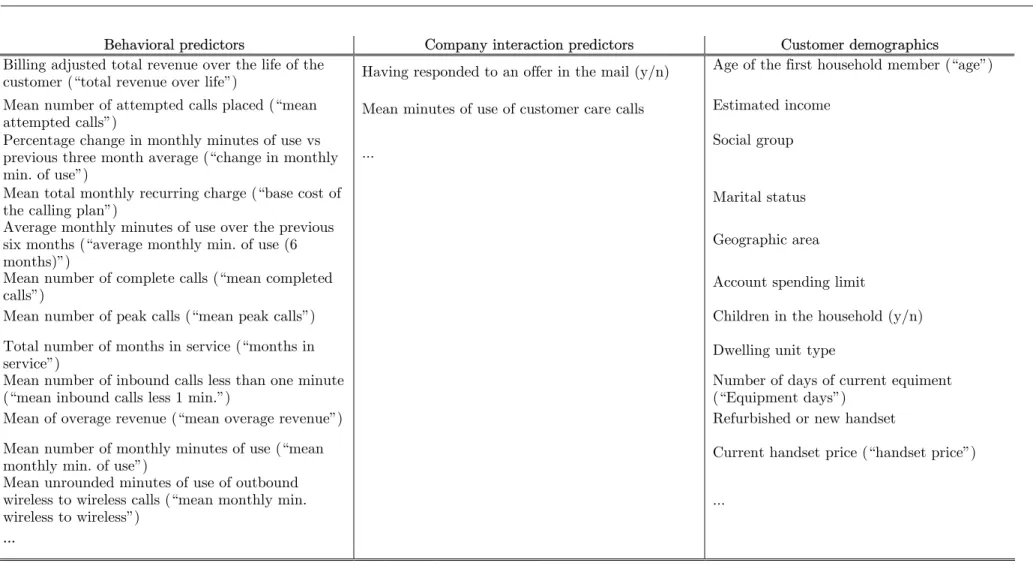
To predict the churn potential of customers, U.S. wireless operators usually take into account between 50 and 300 subscriber variables as explicative factors (Hawley 2003). From the high number of explicative variables contained in the initial database (171 variables), we retain 46 variables, including 31 continuous and 15 categorical variables. Retained predictors include behavioral (e.g. the average monthly minutes of use over the previous three months, the total revenue of a customer account, or the base cost of a calling plan), company interaction (e.g. mean unrounded minutes of customer care calls), and customer demographics (e.g. the number of adults in the household, or the education level of the customer) variables (see Table 1 for an overview). The variable selection is done by first excluding all variables containing more than 30% of missing values. Among the remaining variables, we select the potentially most relevant ones, following the results of a principal components analysis.3 Note that, for an equal comparison, we consider the exact same set of variables for all investigated models.
[Insert Table 1 about here]
2 Originally, the second dataset contained 100,000 observations, but its size was reduced (by taking a random
subset from it) to ensure a fair comparison between both calibration samples.
3 As the purpose of this paper is to investigate the comparative performance of different models, we do not go
into further details about the variables selection which was mainly done to reduce computation time. Some experiments indicated that the performance of the classification rules hardly changed regardless a variable selection procedure was implemented or not.
The handling of missing values is operated differently for the continuous and the categorical predictors. For the continuous variables, the missing values are imputed by the mean of the non-missing ones. As not answering a question may be as informative as a specific response, an extra predictor is also added indicating, for each observation, whether at least one imputation has been made. For categorical predictors, an extra level is created for each of them, indicating whether the value was missing or not.
THE BAGGING AND BOOSTING MODELS
Bagging and boosting both originate from the machine learning research community, and are based on principle of classifier aggregation. This idea was inspired by Breiman (1996) who found gains in accuracy by combining several base classifiers, sequentially estimated from perturbed versions of the calibration sample. Among the several possible alternatives of base classifiers, classification trees (also known as CART, Breiman et al. 1984) are a sensible choice (Breiman 1996). Their use is not widespread in marketing literature, exceptions being e.g. Baines et al. (2003), Currim, Meyer and Le (1988), and Haughton and Oulabi (1993), although they are powerful nonparametric methods. Over the recent years, statistical theory has been elaborated to provide a theoretical background to these techniques (e.g. Bühlmann and Yu 2002, for bagging; Friedman, Hastie and Tibshirani 2000, for boosting; Hastie, Tibshirani, and Friedman 2001, for a comprehensive review).
For the sake of conciseness, the following subsection contains a brief description of the bagging algorithm. In the next subsection, we provide further details about the main differences between bagging and stochastic gradient
boosting, one of the most sophisticated versions of boosting so far. In-depth description of this method can be found in Friedman (2002).
Bagging
Bagging (i.e. Bootstrap AGGregatING) is, by far, the simplest technique to upgrade, or to “boost”, the performance of a given choice model. Denote the calibration sample by Z =
{
(
x1,y1)
,K,(
xi,yi)
,K,(
xN,yN)
}
, where N is the number of customers in the calibration sample. In this expression,) ,..., ,...,
( i1 ik iK
i x x x
x = represents a vector containing the K predictors for customer i , while yi (equal to 1 or —1) indicates whether this customer i will
churn or not. A base classifier fˆ is estimated from this calibration sample, giving
a score value fˆ
( )
x to each customer, with x the characteristics of this subscriber. This score value indicates the risk to churn associated with each customer. For a specified cut-off value τ , customers can be predicted as churners or non-churners by computing( )
(
−τ)
= signf x x cˆ( ) ˆ , (1)returning values +1 or —1. If fˆ
( )
xi is larger than τ , customer i will be classified as a churner, while, if f( )
xi is smaller than τ , the customer will be predicted asa non-churner. When using a classification tree as base classifier, the score is given by fˆ
( )
x =2pˆ( )
x −1, where pˆ( )
x is the probability to churn as estimated by the tree. When working with a proportional calibration sample, we set τ =0. In the presence of a non-proportional calibration sample, the value of τ varies (see next section).From the original calibration set Z , we construct B bootstrap samples B b Zb, 1,2, , * K
= , by randomly drawing, with replacement, N observations from
Z . Note that the size of the bootstrap samples equals the original calibration sample size. From each bootstrap sample Zb*, a base classifier is estimated, giving
B score functions f
( )
x fb( )
x fB( )
x* *
*
1 , ,ˆ , , ˆ
ˆ K K . These functions are then aggregated
into the final score
( )
∑
= = B b b bag f x B x f 1 * ˆ 1 ) ( ˆ . (2)Classification can then be carried out via
(
bag B)
bag x signf x
cˆ ( )= ˆ ( )−τ , with cˆbag(x)∈
{
−1,1}
. (3) Again, the cut-off value τB equals zero in the presence of a proportionalcalibration sample. To determine the optimal value of B (i.e. the number of bootstrap samples), a strategy consists in selecting B such that the apparent error rates4 (i.e. error rates on the calibration data) remain as good as constant for values larger than B . In our application, we set B =100.
Like for traditional classification models, diagnostics measures can also be obtained for the estimated bagging model. These are important to give some face validity to the estimated model. For instance, one may investigate the estimated relative importance of each predictor in the construction of the classification rule. For a single tree, the relative importance of a predictor can be computed as in
Hastie, Tibshirani and Friedman (2001).5 For bagging (and similarly for boosting), the relative importance of an explicative variable is simply averaged over all B trees. Also the partial dependence of churn on a specified predictor variable can be investigated. This measure provides similar insight than the parameters’ estimates value of a logit model, but advantageously allows for non-linear relationships between the predictors and the dependent variable. A partial dependence plot represents the impact of a predictor variable on the churn probability of a customer, conditional on all other predictors. In practice, the partial dependence of the dependent variable on a specified value of a predictor
k
x is obtained by assigning this value of xk to all observations of the calibration sample. The model is subsequently estimated, and the N resulting predicted probabilities computed for the calibration data. The partial dependence on a specified value of xk is eventually given by averaging over these N predicted
probabilities. The partial dependence plot is obtained by letting the value assigned to xk varies over a large range of values (for more details, see Friedman
2001).
Boosting and Stochastic Gradient Boosting
Several versions of boosting exist, e.g. the real adaboost (Freund and Schapire 1996; Schapire and Singer 1999), logitboost (Friedman, Hastie and Tibshirani 2000), or gradient boosting (Friedman 2001). Boosting is more complex than bagging, and less easy to put into practice. In this paper, we focus on
5 More precisely, a tree is composed of several nodes, from the root to the leaves (i.e. terminal nodes). Each
non-terminal node is split into two child nodes on the basis of the value of the variable providing the
maximal reduction in the squared error rate. The relative importance of a variable xk is then the sum of these
stochastic gradient boosting6 (Friedman 2002), one of the most recent boosting variants, and the winning model of the Teradata Churn Modeling Tournament (Cardell, Golovnya and Steinberg 2003).
The main difference between boosting and the above described bagging procedure basically lies in the sampling scheme. Boosting consists in sequentially estimating a classifier to adaptively reweighted versions of the initial calibration sample Zb, b 1, 2, ..., B
* =
. The adaptive reweighting scheme enables to give previously misclassified customers an increased weight on the next iteration, while weights given to previously correctly classified observations are reduced. The idea is to force the classification procedure to concentrate on the hard-to-classify customers.
Another main difference with bagging is that the initial choice model should preferably be “weak”, i.e. with a slightly lower associated error rate than random guessing. For stochastic gradient boosting, Friedman (2002) advised to use k-node trees as base classifier where k is about 6 to 9, depending on the issue. Also the number of required iterations is usually higher for stochastic gradient boosting than for bagging. In our application, we select B =1000.
CORRECTION FOR A BALANCED SAMPLING SCHEME
Predictions made from a model estimated on a balanced calibration sample are known to be biased as they overestimate the proportion of churners in real-life. While appropriate bias correction methods already exist for some common classifiers (see e.g. King and Zeng 2001b for the logit model), to the best of our knowledge, there does not exist (yet) any correction method for bagging and
boosting. Hereafter, we adapt to the bagging and boosting models two simple bias correction methods discussed by King and Zeng (2001b).
The first correction consists in attaching a weight to each observation of the balanced sample. These weights are based on marketers’ prior beliefs about the churn rate πc , i.e. the proportion of churners, among their customers. For
example, πc can be taken as the empirical frequency of churners in a proportional
sample, in our case 1.8%. Let Ncbalanced be the number of churners in the balanced
sample, with N the total size of this sample. One may weight observations of a balanced calibration sample by attaching the weights
balanced c c nc i balanced c c c i N N w N w − − = = π and 1 π (4)
to the churners, respectively the non-churners. As such, the sum of the weights associated to the churners equals the real-life proportion of churners. Note that the sum of the weights defined in (4) is always equal to one. When applying this weighting correction to bagging and stochastic gradient boosting, a sequence of weighted decision trees is estimated, where the weights remain fixed through iterations. Statistically speaking, assigning weights to customers is a valid approach to correct for stratified sampling. However, since the weights assigned to the churners will be small, one could fear that this correction would actually cancel the advantage of oversampling the churners, and would provide similar results as a proportional sample of the same size (see Results section).
Rather than weighting the observations of a balanced sample, a more simple approach is to take a non-zero cut-off value τB in the bagging and
boosting algorithms. The value of τB is taken such that the proportion of
predicted churners in the calibration sample equals the actual a priori proportion of churners πc . This correction is achieved for bagging (and similarly for
boosting) by first sorting the values of fˆbag(x) in the calibration sample from the
largest to the smallest value, fˆbag
( )
x( )1 ≥fˆbag( )
x( )2 ≥K≥fˆbag( )
x( )N , and taking( )
( )
ˆ j bag B =f x τ , with j = Nπc. (5)This latter correction method can also be called intercept correction (or prior correction as in King and Zeng 2001a,b), by analogy to a similar correction for the logit model (see e.g. Franses and Paap 2001, pp. 73-75). Unlike the weighting correction, the intercept correction does not affect the estimated scores, nor the ranking of the customers. Both corrections are assessed in the Results section.
ASSESSMENT CRITERIA
The predictive performance of the investigated models is assessed using a hold-out test sample (as described in the Data section). As this sample has not been used for estimating the classification rules and is very large, it allows for a valid assessment of performance. Denote
{
(
x1,y1)
,K,(
xi,yi)
,K,(
xM,yM)
}
the validation or hold-out test sample. The computed scores are denoted by fˆ( )
xi ,for i =1,K,M where M is the size of the validation sample.
Error rate
The traditional performance criterion is the error rate, counting the percentage of incorrectly classified observations in the validation set. For rare
events, the error rate is often inappropriate, as already noticed by Morrison (1969). For instance, a naïve prediction rule stating that no customer of the validation set churns has an expected error rate of approximately 1.8%, from which the classification rule could be falsely considered as good. Indeed, such a rule does not isolate any group of potentially riskiest customers for undertaking a targeted retention strategy. As another drawback, error rates do not take the numerical values of the scores fˆ
( )
xi into account, while the latter may containrelevant information for proactive marketing actions. The targeting of such incentives can indeed be based on the churn degree of risk (i.e. score) of each customer, e.g. targeting the 10% most risky customers. The top-decile lift and the gini coefficient, in contrast, are based on these scores.
Top-decile lift
The top-decile lift focuses on the most critical group of customers regarding their churn risk. The top 10% riskiest customers (i.e. those having score values among the 10% highest) is potentially an ideal segment for targeting a retention marketing campaign. The top-decile lift equals the proportion of churners in this
risky segment, πˆ10%, divided by the proportion of churners in the whole validation
set, πˆ: π π ˆ ˆ10% = decile Top . (6)
The higher the top-decile lift, the better the classifier. This measure enables to control whether the targeted segment of risky customers indeed contains actual churners. As extensively described by Neslin et al. (2004),
top-decile lift is related directly to profitability. They define the incremental gain in financial profit from an increase in top-decile lift as
(
)
(
γ δ(
γ ψ)
)
π
α ∆ − −
=N Topdecile LVC
Gain ˆ (7)
where N is the customer base of the company, α is the percentage of targeted customers (here, 10%), ∆Topdecile is the increase in top-decile lift, γ is the success rate of the incentive among the churners, LVC is the lifetime value of a customer (Gupta, Lehmann and Stuart 2004), δ is the incentive cost per customer, and ψ is the success rate of the incentive among the non-churners (for more details, see Neslin et al. 2004).
Gini coefficient
Another interesting measure is the gini coefficient (e.g. Hand 1997, p.134). Instead of only focusing on the most risky segment, this measure considers all scores, including also the less risky customers. The top-decile lift and the gini coefficient give complementary information; a model can be good at identifying the riskiest segment, but weaker at recognizing less risky customers. We first determine the fraction of all subscribers having a predicted churn probability above a certain threshold. A whole sequence of thresholds is considered, each of them given by a predicted score fˆ
( )
xl , for l =1,2,...,M, resulting in Mproportions
( )
( )
[
]
∑
= > = M i l i l I f x f x M 1 ˆ ˆ 1 π . (8)For each threshold, the fraction of all churners having score value above this threshold is also computed
( )
( )
[
]
∑
= = > = ′ Mc i i l i c l I f x f x y M 1 1 and ˆ ˆ 1 π , (9)with Mc the total number of actual churners in the validation set. The gini
coefficient is then defined as
(
)
∑
= − ′ = M l l l M t coefficien Gini 1 2 π π . (10)The larger the gini coefficient, the better the classification model would be.
RESULTS
This section addresses the research questions exposed in the Introduction section. We show that (i) both bagging and boosting techniques significantly improve the classification performance of traditional classification models, that (ii) the correction methods for a balanced calibration sample reduces the classification error rate, and that (iii) the use of a balanced calibration sample improves the forecasting accuracy of the estimated choice models.
Q.1 Do bagging and boosting provide better results than other
benchmarks?
We first apply bagging and stochastic gradient boosting7 — with classification trees as base classifiers — to the balanced calibration sample. As a benchmark, we estimate a binary logit choice model on the same sample. Other
benchmark models are also investigated, including the traditional discriminant analysis, a single classification tree and a neural network (see e.g. Thieme, Song and Calantone 2000; West, Brockett and Golden 1997), but appear to perform worse that the binary logit choice model in this empirical application. Neslin et al. (2004) have recently compared the predictive performance of different methodological approaches for this particular database and have found the logit model and the decision tree to be among the most competitive methodologies used. To evaluate the relative performance of the different methods, we apply the estimated models to the hold-out proportional test sample in order to obtain churn predictions for each of the customers belonging to this latter sample. From these predictions, we then compute the validated error rate, the gini coefficient and the top-decile lift reached by each of the three choice models.
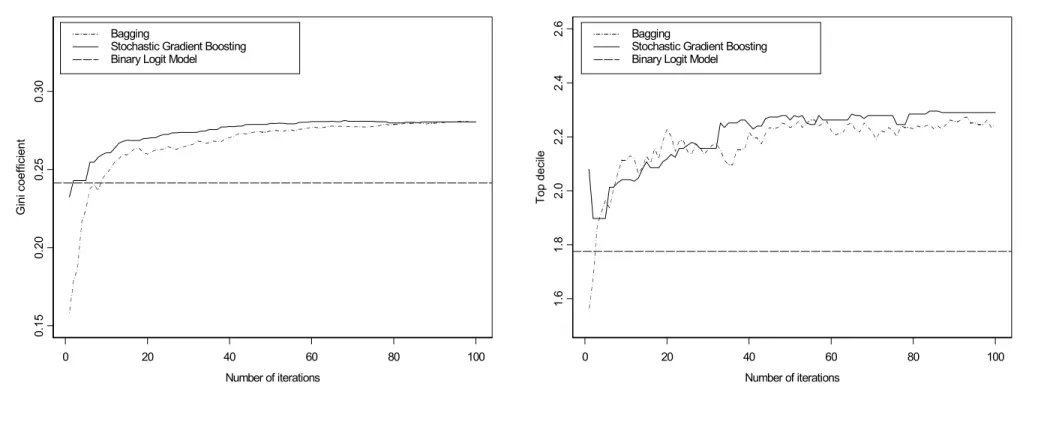
[Insert Figure 1 about here]
Figure 1 represents the gini coefficient and the top-decile lift against the number of iterations for both bagging and stochastic gradient boosting.8 The horizontal line in Figure 1 represents the performance of the binary logit model. The performance of bagging and boosting improves as B increases, and stabilizes for large values of B. After a first few iterations, both models already outperform the logit benchmark,9 confirming hereby many other examples (e.g. Hastie, Tibshirani and Friedman 2001, pp.246-249 & 299-345).
7 Bagging was implemented in the statistical software package Splus, while stochastic gradient boosting was
computed with the MART software package for R developed by J.H. Friedman.
8 Note that B is actually multiplied by 10 for stochastic gradient boosting in Figure 1.
9 The gini coefficient and top-decile lift are respectively -0.06 and 0.49 for neural nets, 0.199 and 1.60 for
discriminant analysis, and 0.091 and 1.37 for a single classification tree, compared to 0.24 and 1.77 for logit regression. These figures motivate our preference for the logit model as benchmark.
The relative gain in predictive performance is greater than 16% for the gini coefficient, and 26% for the top-decile lift. Statistically speaking, this improvement is significant.10 Stochastic gradient boosting performs very comparatively to bagging, but is conceptually more complicated. Therefore, we consider bagging as the most competitive approach, at least in this application. We may also evaluate the additional financial gains (7) that we may expect from a retention marketing campaign which would be targeted using the scores predicted by the bagging instead of the logit model. If we consider N = 5,000,000 customers, a target group of α = 10%, γ = 30% success probability among the churners, LVC =$2,500 lifetime value, δ =$50 incentive cost and ψ=50% success probability among the non-churners, then using bagging as scoring model — instead of a logit model — for targeting a specific retention campaign is worth an additional $3,214,800.
Regarding the error rate, all the three choice models perform quite poorly (see Table 2; third column), confirming that a balanced sampling scheme requires an appropriate bias correction, regardless of the choice model under consideration. In the next research question, we investigate whether a bias correction reduces these high error rates.
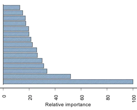
Although the bagging and boosting models mainly focus on scoring customers for targeting purposes, the models can also interpreted. Figure 2 reports the fifteen most important variables in explaining churn, using bagging.11 Reported results offer some face validity. Among the particularly relevant churn triggers, we find the number of days of the current cell phone (“equipment
10 Standard errors (computed by a bootstrap procedure) are about 0.012 for the gini coefficient and 0.09 for
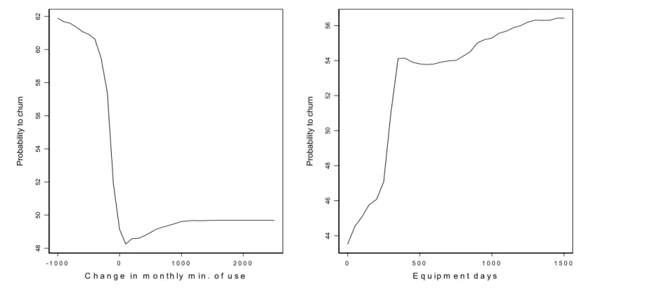
days”), the changes in minutes’ consumption over the previous three months (“change in monthly min. of use”), as well as the base cost of the calling plan chosen by the customer (“base cost of the calling plan”). Partial dependence plots provide additional insights on the way these variables affect churn.
[Insert Figure 2 and Figure 3 about here]
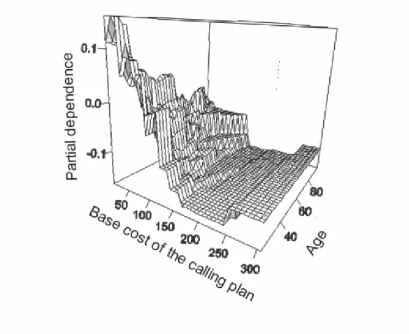
It appears that (Figure 3; right panel) the probability that a customer churns increases as his cell phone becomes older. This rise is particularly important around one year, which could be explained as numerous operators propose combined one-year-subscription and free cell phone packages. After this delay, customers may be likely to defect the company and buy a new package from a competitor. Figure 3 (left panel) indicates how the churn risk of a customer varies as his consumption habits change. When his consumption decreases, a subscriber would be more likely to churn. When his consumption is about constant, he would be less likely to defect. Finally, when his consumption increases, he would be slightly less (but still) likely to be loyal than when no change occurs.12 Another interesting insight can be derived from Figure 4, which represents the partial dependence between churn and a combination of two churn drivers, i.e. the age of the customer (“age”) and the base cost of his calling plan. A customer is found to be more likely to churn when his calling plan would be cheaper. However, this relationship tends to be much stronger for younger customers than older ones, indicating that some demographics are more likely to drop certain calling plans than others.
[Insert Figure 4 about here]
Q.2 What is the best bias correction when using a balanced calibration
sample?
Two corrections are envisaged to adapt the predicted probabilities obtained by using a balanced calibration sample. Using any of these two corrections reduces the error rate significantly, as illustrated in Table 2.
[Insert Table 2 about here]
The effectiveness of both corrections differs. Regarding the error rate, the weighting correction seems the most appropriate bias correction method for all considered models. However, the weighting correction affects the estimated scores, as well as their ranking, and eventually the gini coefficient and the top-decile lift. This is not the case for the intercept correction method which preserves the relative ranking of the attributed scores. Table 3 reports the gini coefficient and the top-decile lift for bagging, stochastic gradient boosting, and the logit model (all estimated on the balanced sample), for both corrections. The gini coefficient and the top-decile lift reached by the intercept correction are substantially better than those using the weighting correction, for all the three models under consideration.
[Insert Table 3 about here]
This confirms the prior assumption that weighting the observations of a balanced sample cancels the advantage of balanced sampling, even for large sample sizes. As we consider the gini coefficient and the top-decile lift as more global measures of performance than the error rate, the intercept correction is
found to be — at least in this application — the best compromise between no correction (i.e. better gini coefficient and top-decile lift, but worse error rate) and weighting correction (i.e. worse gini coefficient and top-decile lift, but better error rate).
Note that the intercept correction appears to perform well for stable markets (e.g. constant churn rate), but is likely to be inefficient in dynamic markets (e.g. increasing churn rate). This constitutes a major limitation to the correction methods proposed in this study. Moreover, the lack of theory regarding the properties of these correction methods prevents us from generalizing our findings to any other setting.
Q.3 Does a choice model estimated on a balanced sample, and
appropriately corrected for the bias, outperform a choice model estimated
on a proportional sample?
It is often advised to use a balanced calibration sample when the variable to be predicted consists of a rare event, like churn. This third research issue puts this statement into question. Indeed, given the high amount of observations in the proportional calibration sample, the absolute number of churners is still quite large, and a proportional sampling could still be efficient.
[Insert Table 4 about here]
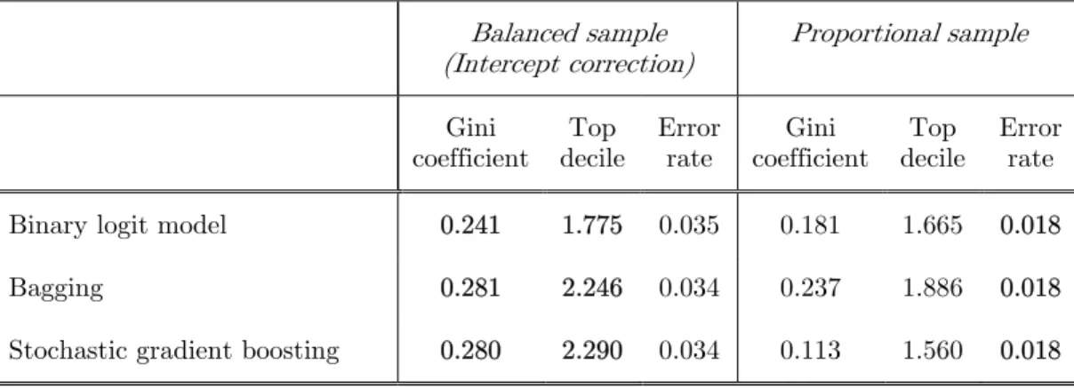
Table 4 compares the performance of bagging, stochastic gradient boosting and the binary logit model, estimated from the proportional or the balanced sample (with intercept correction). Results on the gini coefficient and top-decile lift both indicate that the balanced sampling scheme is recommended for the three
investigated classification models. For the error rate, results are more in favor of the proportional sampling. However, for the same reasons as in Q.2, we consider the balanced sampling as a better compromise that the proportional sampling which poorly perform regarding gini coefficient and top-decile lift.
CONCLUSIONS AND FURTHER RESEACH
In this paper, we have brought some new developments originating from machine learning and statistical classification literature to the attention of marketing researchers. We have presented one of the simplest versions of classifier aggregation, i.e. bagging, as well as one of the most sophisticated algorithms in this field, i.e. stochastic gradient boosting. Attention has especially been drawn on the very competitive performance of bagging, an easy-to-use procedure aimed at increasing the classification performance of an initial classification model, by repeatedly estimating a classifier to bootstrapped versions of the calibration sample. We summarize the main findings of this study in three contributions.
1. Bagging and boosting provide substantially better classifiers than a binary logit model. In predicting churn, the gain in predictive performance has reached 16% for the gini coefficient, and 26% for the top-decile lift. Bagging and stochastic gradient boosting perform very comparatively. The performance of the very simple and easy-to-use bagging is especially noticeable. Besides their higher predictive power, bagging and boosting also provide good diagnostic measures, variables’ importance and partial dependence plots, which offer some face validity to the models and interesting insights about potential churn drivers.
2. In the presence of a rare event like churn, a balanced sampling scheme is recommended and preferred to proportional sampling for all considered
classification models (i.e. bagging, boosting and logit models), even for large datasets. However, to maintain the classification error rate at a reasonable level, it is necessary to correct the predictions obtained from a balanced sample.
3. Intercept correction constitutes an appropriate bias correction for balanced sampling scheme.
If companies take into account these recommendations, they should be able to better identify the riskiest customers’ segment in terms of churn risk, and therefore ameliorate their retention strategy. Noteworthy losses could ultimately be avoided.
Table 1: Description of the churn predictors
Behavioral predictors Company interaction predictors Customer demographics
Billing adjusted total revenue over the life of the
customer (“total revenue over life”) Having responded to an offer in the mail (y/n)
Age of the first household member (“age”) Mean number of attempted calls placed (“mean
attempted calls”) Mean minutes of use of customer care calls
Estimated income Percentage change in monthly minutes of use vs
previous three month average (“change in monthly min. of use”)
... Social group
Mean total monthly recurring charge (“base cost of
the calling plan”) Marital status
Average monthly minutes of use over the previous six months (“average monthly min. of use (6 months)”)
Geographic area
Mean number of complete calls (“mean completed
calls”) Account spending limit
Mean number of peak calls (“mean peak calls”) Children in the household (y/n)
Total number of months in service (“months in
service”) Dwelling unit type
Mean number of inbound calls less than one minute (“mean inbound calls less 1 min.”)
Number of days of current equiment (“Equipment days”)
Mean of overage revenue (“mean overage revenue”) Refurbished or new handset
Mean number of monthly minutes of use (“mean
monthly min. of use”) Current handset price (“handset price”)
Mean unrounded minutes of use of outbound wireless to wireless calls (“mean monthly min. wireless to wireless”)
... ...
Figure 1: Validated gini coefficient (left) and top-decile lift (right) for bagging, stochastic gradient boosting and a binary logit model as a function of B 0 20 40 60 80 100 Number of iterations 0. 1 5 0. 2 0 0. 25 0. 30 G ini c o ef fic ien t Bagging
Stochastic Gradient Boosting Binary Logit Model
0 20 40 60 80 100 Number of iterations 1. 6 1 .8 2. 0 2.2 2. 4 2.6 T op de cile Bagging
Stochastic Gradient Boosting Binary Logit Model
Figure 2: Variables’ relative importance for bagging
0 20 40 60 80
10
0
Equipment days Change in monthly min. of useBase cost of the calling plan Handset price Mean peak calls Total revenue over life Mean overage revenue Average monthly min. of use (6 months)Mean completed calls Months in service Mean attempted calls Mean monthly min. of useAge Mean monthly min. wireless to wirelessMean inbound calls less 1 min.
Figure 3: Partial dependence plots for “change in monthly min. of use” and “equipment days” for bagging - 1 0 0 0 0 1 0 0 0 2 0 0 0 C h a n g e in m o n t h ly m in . o f u s e 48 50 52 54 56 58 60 62 Pr o ba bilit y t o c hu rn 0 5 0 0 1 0 0 0 1 5 0 0 E q u ip m e n t d a y s 44 46 48 50 52 54 56 Pr o ba bilit y t o c hu rn
Table 2: Validated error for predicting churn from a balanced sample with intercept correction, weighting correction or without bias correction.
Error rate Intercept correction
Weighting correction
No correction
Binary logit model 0.035 0.018 0.400
Bagging 0.034 0.025 0.374
Stochastic gradient boosting 0.034 0.018 0.460
Table 3: Validated gini coefficient and top-decile lift for predicting churn from a balanced sample with intercept correction and weighting correction
Intercept correction (∗) Weighting correction Gini coefficient Top decile Gini coefficient Top decile
Binary logit model 0.241 1.775 0.239 1.764
Bagging 0.281 2.246 0.161 1.549
Stochastic gradient boosting 0.280 2.290 0.187 1.632
(∗) These gini coefficients and top-decile lifts are the same for the “no correction” method.
Table 4: Validated gini coefficient, top-decile lift and error rate with a balanced and a proportional calibration sampling.
Balanced sample (Intercept correction) Proportional sample Gini coefficient Top decile Error rate Gini coefficient Top decile Error rate Binary logit model 0.241 1.775 0.035 0.181 1.665 0.018
Bagging 0.281 2.246 0.034 0.237 1.886 0.018
REFERENCES
Andrews, Rick L., Andrew Ainslie, and Imram S. Currim (2002), “An Empirical Comparison of Logit Choice Models with Discrete Versus Continuous Representations of
Heterogeneity,” Journal of Marketing Research, 39, 479-487.
Andrews, Rick L. and Imran S. Currim (2002), “Identifying Segments with Identical Choice Behaviors Across Product Categories: An Intercategory Logit Mixture Model,”
International Journal of Research in Marketing, 19, 65-79.
Arora, Neeraj, Greg M. Allenby, and James L. Ginter (1998), “A Hierarchical Bayes
Model of Primary and Secondary Demand,” Marketing Science, 17, 29-44.
Athanassopoulos, Antreas D. (2000), “Customer Satisfaction Cues to Support Market
Segmentation and Explain Switching Behavior,” Journal of Business Research, 47,
191-207.
Baines, Paul R., Robert M. Worcester, Jarrett David, and Roger Mortimore (2003), “Market Segmentation and Product Differentiation in Political Campaigns: A Technical
Feature Perspective,” Journal of Marketing Management, 19, 225-249.
Bhattacharya, C.B. (1998), “When Customers are Members: Customer Retention in Paid
Membership Contexts,” Journal of the Academy of Marketing Science, 26, 31-44.
Bolton, Ruth N., P.K. Kannan and Matthew D. Bramlett (2000), “Implications of Loyalty Program Membership and Service Experiences for Customer Retention and
Value,” Journal of the Academy of Marketing Science, 28, 95-108.
Breiman, Leo (1996), “Bagging Predictors,” Machine Learning, 26, 123-140.
---, Jerome H. Friedman, Richard A. Olshen, and Charles .J. Stone (1984), Classification
and Regression Trees, New York: Chapman and Hall.
Bühlmann, Peter and Bin Yu. (2002), “Analyzing Bagging,” Annals of Statistics, 30,
927-961.
Cardell, Scott N., Mikhail Golovnya, and Dan Steinberg (2003), “Churn Modeling for Mobile Telecommunications: Winning the NCR Teradata Center for CRM at Duke
University - Salford Systems,” 2003INFORMS Marketing Science Conference, Maryland.
Chung, Jaihak and Vithala R. Rao (2004), “A General Choice Model for Bundles with Multiple-Category Products: Application to Market Segmentation and Optimal Pricing
for Bundles,” Journal of Marketing Research, 41, 115-130.
Colgate, Mark R. and Peter J. Danaher (2000), “Implementing a Customer Relationship
Strategy: The Asymmetric Impact of Poor versus Excellent Execution,” Journal of the
Academy of Marketing Science, 28, 375-387.
Corstjens, Marcel L. and David A. Gautschi (1983), “Formal Choice Models in
Marketing,” Marketing Science, 2, 19-56.
Cosslett, S.R. (1993), “Estimation from Endogenously Stratified Samples,” in Handbook
of Statistics, Maddala G.S., C.R. Rao and H.D. Vinod, eds. Amsterdam: Elsevier Science Publishers.
Currim, Imran S., Robert J. Meyer, and Nhan T. Le (1988), “Disaggregate
Tree-Structure Modelling of Consumer Choice Data,” Journal of Marketing Research, 25,
253-265.
Donkers, Bas, Philip H.B.F. Franses, and Peter Verhoef (2003), “Selective Sampling for
Binary Choice Models,” Journal of Marketing Research, 40, 492-497.
Donkers, Bas, Richard Paap, Jedid-Jah Jonker, and Philip H.B.F. Franses (2005),
“Deriving Target Selection Rules from Endogenously Selected Samples,” Journal of
Applied Econometrics, forthcoming.
Franses, Philip H. and Richard Paap (2001), Quantitative Models for Marketing
Research, Cambridge: Cambridge University Press.
Freund, Yoav and Robert E. Schapire (1996), “Experiments with a New Boosting
Algorithm,” In Proceedings of the 13th International Conference on Machine Learning,
148-156.
Friedman, Jerome H. (2001), “Greedy Function Approximation: A Gradient Boosting
Machine”, The Annals of Statistics, 29, 1189-1232.
---- (2002), “Stochastic Gradient Boosting”, Computational Statistics and Data Analysis,
38, 367-378
----, Trevor Hastie, and Robert Tibshirani (2000), “Additive Logistic Regression: a
Statistical View of Boosting,” The Annals of Statistics, 28, 337-407.
Ganesh, Jaishankar, Mark J. Arnold, and Kristy E. Reynolds (2000), “Understanding the Customer Base of Service Providers: An Examination of the Differences between
Switchers and Stayers,” Journal of Marketing, 65, 65-87.
Guadagni, Peter M. and John D.C. Little (1983), “A Logit Model of Brand Choice
Calibrated on Scanner Data,” Marketing Science, 2, 203-238.
Gupta, Sunil, Donald R. Lehmann, and Jennifer A. Stuart (2004), “Valuing Customers,”
Journal of Marketing Research, 16, 7-18.
Hand, David J. (1997), Construction and Assessment of Classification Rules, Chichester:
Wiley Series in Probability and Statistics.
Hastie, Trevor, Robert Tibshirani, and Jerome Friedman (2001), The Elements of
Statistical Learning: Data Mining, Inference and Prediction, New York: Springer-Verlag. Haughton, Dominique and Samer Oulabi (1993), “Direct marketing modeling with CART
and CHAID,” Journal of Direct Marketing, 7, 16- 26.
Hawley, David (2003), “International Wireless Churn Management Research and
Recommendations,” Yankee Group report, June.
Imbens, Guido W. and Tony Lancaster (1996), “Efficient Estimation and Stratified
Sampling,” Journal of Econometrics, 74, 289-318.
Kalwani, Manohar U., Robert J. Meyer, and Donald G. Morrison (1994), “Benchmarks
King, Gary and Langsche Zeng (2001a), “Explaining Rare Events in International
Relations,” International Organization, 55, 693-715.
King, Gary and Langsche Zeng (2001b), “Logistic Regression in Rare Events Data,”
Political Analysis, 9, 137-163.
Morrison, Donald G. (1969), “On the Interpretability of Discriminant Analysis,” Journal
of Marketing Research, 6, 156-163.
Nardiello, Pio, Fabrizio Sebastiani, and Alessandro Sperduti (2003), “Discretizing
Continuous Attributes in AdaBoost for Text Categorization,” Proceedings of ECIR-03,
25th European Conference on Information Retrieval, Pisa, 320-334.
Neslin, Scott A., Sunil Gupta, Wagner Kamakura, Junxiang Lu, and Charlotte Mason (2004), “Defection Detection: Improving Predictive Accuracy of Customer Churn
Models,” Working Paper Series, Teradata Center for Customer Relationship Management
at Duke University.
Schapire, Robert E. and Yoram Singer (1999), “Improved Boosting Algorithms using
Confidence-rated Predictions,” Machine Learning, 37, 297-336.
Scott, Alastair J. and Chris J. Wild (1997), “Fitting Regression Models to Case-Control
Data by Maximum Likelihood,” Biometrika, 84, 57-71.
Shaffer, Greg and John Z. Zhang (2002), “Competitive One-to-One Promotions,”
Management Science, 48, 1143-1160.
The Wall Street Journal Europe (2000), “Fighting the Fickle,” September 18.
Thieme, R. Jeffrey, Michael Song, and Roger J. Calantone (2000), “Artificial Neural Network Decision Support Systems for New Product Development Project Selection,”
Journal of Marketing Research,37, 499-507.
Varmuza, Kurt, Ping He, and Kai-Tai Fang (2003), “Boosting Applied to Classification
of Mass Spectral Data,” Journal of Data Science, 1, 391-404.
Viaene, Stijn, Richard A. Derrig and Guido Dedene (2002). “Boosting Naive Bayes for
Claim Fraud Diagnosis,” in Lecture Notes in Computer Science 2454, Berlin: Springer.
Wedel, Michel and Wagner A. Kamakura (2000), Market Segmentation: Conceptual and
Methodological Foundations, 2d ed. Boston: Kluwer Academic Publishers.
West, Patricia M., Patrick L. Brockett, and Linda L. Golden (1997), “A Comparative Analysis of Neural Networks and Statistical Methods for Predicting Consumer Choice,”
Marketing Science, 16, 370-391.
Yang, Sha and Greg M. Allenby (2003), “Modeling Interdependent Consumer