The contribution of various physical sources of uncertainty affecting radar rainfall estimates at the ground is quantified toward deriving and understanding the error covariance matrix of these estimates. The focus here is on stratiform precipitation at a resolution of 15 km, which is most relevant for data assimilation onto mesoscale numerical models. In the characterization of the error structure, the following contributions are considered: (i) the individual effect of the range-dependent error (associated with beam broadening and increasing height of radar measurements with range), (ii) the error associated with the transformation from reflectivity to rain rate due to the variability of drop size distributions, and (iii) the interaction of the first two, that is, the term resulting from the cross correlation between the effects of the range-dependent error and the uncertainty related to the variability of drop size distributions (DSDs).
For this purpose a large database of S-band radar observations at short range (where reflectivity near the ground is measured and the beam is narrow) is used to characterize the range-dependent error within a simulation framework, and disdrometric measurements collocated with the radar data are used to assess the impact of the variability of DSDs. It is noted that these two sources of error are well correlated in the vicinity of the melting layer as result of the physical processes that determine the density of snow (e.g., riming), which affect both the DSD variability and the vertical profile of reflectivity.
1. Introduction
In recent years, an effort has been made to assimilate radar observations (of both reflectivity and radial ve-locity) into numerical weather prediction (NWP) mod-els (see the reviews of Errico et al. 2000; MacPherson et al. 2003; Sun and Wilson 2003; Sun 2005a). Moreover, as the resolution of NWP models increases, denser ob-servations are required for assimilation, and the reso-lution and coverage of data from radar networks make them very attractive for this purpose.
From the perspective of the assimilation of radar rainfall observations in NWP models, two main lines of work can be identified:
• schemes assimilating surface rainfall measurements, mainly to constrain the profiles of temperature and specific humidity at meso-␣ to synoptic scales
(Županski and Mesinger 1995; Fillion and Errico 1997; Guo et al. 2000; Marecal and Mahfouf 2000; MacPherson 2001; Deblonde et al. 2007), and • schemes assimilating volumetric reflectivity
observa-tions to constrain the rainwater mixing ratio (Sun and Crook 1997; Montmerle et al. 2001; Crook and Sun 2002; Caya et al. 2005; Sun 2005b; Chung et al. 2007; Hu and Xue 2007; Xiao et al. 2007). These models (which can include a complete description of the mi-crophysics or simplified parameterizations) are typi-cally run at convective scale, though some attempts have been made at larger scales as well (Sun and Wilson 2003).
The works mentioned above show the beneficial effects of assimilating radar rainfall measurements into NWP models using variational methods in any of their configurations [one-dimensional variational data assimilation (1DVAR), 3DVAR, or 4DVAR] or the ensemble Kalman filter (EnKF).
Variational methods are based on a least squares– like approach, which consists of minimizing a cost
func-Corresponding author address: Marc Berenguer, 805 Sher-brooke St. West, Montreal, QC H3A2K6, Canada.
E-mail: [email protected] DOI: 10.1175/2008WAF2222134.1 © 2008 American Meteorological Society
tion of the following type (see, e.g., Daley 1991; Kalnay 2003): J共x兲⫽1 2共x⫺xb兲 TB⫺1共 x⫺xb兲 ⫹1 2关H共x兲⫺yo兴 T R⫺1关H共x兲⫺yo兴, 共1兲
where x, xb, and yoare the analysis, the background, and the observation vectors, respectively, and H( ) is the observation operator, which relates model variables with observations. The accuracies of the background term and observations are represented byBandR, that is, the background and observation error covariance matrices, respectively. The quality of the approxima-tions ofBandRused in the assimilation schemes have a significant impact on their performance.
It has been pointed out (Errico et al. 2000; MacPher-son et al. 2003; Sun 2005a; Xu et al. 2007) that one important limitation of the schemes assimilating pre-cipitation observations lies in the simplifications as-sumed to describe observational errors (either using variational methods or, similarly, the EnKF). Within this framework, the present work focuses on the char-acterization of the observation error covariance matrix of radar rainfall estimates at the ground for assimilation in mesoscale models. Given the large variability of pre-cipitation processes, we emphasize the detailed under-standing of the sources of these errors so that the error covariance matrix can be made adaptive to precipita-tion types.
Specifically, the main goal of this study is to charac-terize the variability and correlation of the errors af-fecting radar estimates of surface rainfall in stratiform conditions by analyzing in detail the physical factors affecting the error structure, and to test the validity of assuming these errors homogeneous or uncorrelated, which are the usual hypotheses in most of the current assimilation schemes.
The different sources of uncertainty affecting radar rainfall estimates have been discussed by several au-thors (e.g., Wilson and Brandes 1979; Zawadzki 1984; Austin 1987; Joss and Waldvogel 1990), and works quantifying their impact can be found in the radar lit-erature. However, the variability of these errors and their spatial and temporal correlation (necessary to fully characterize the error covariance matrix of radar rainfall observations) had only recently been consid-ered. In this sense, Germann et al. (2006) point out two different approaches in the characterization of the error covariance matrix of radar estimates of rain intensity at the ground:
• those based on comparing radar rainfall estimates with reference measurements (typically, rain gauge observations), considered to be free of error and as-suming that the variability and structure of their re-siduals are entirely attributable to radar errors (Ciach et al. 2007; Germann et al. 2008, manuscript submit-ted toQuart. J. Roy. Meteor. Soc., hereafter GBSTZ); and
• those based on studying the individual impact of the most relevant sources of error, by simulating the er-rors with conceptual physical models and/or experi-mental data [see the simplified approach of Jordan et al. (2003), and the detailed analysis of individual er-rors of Bellon et al. (2005) and Lee and Zawadzki (2005)], and the interaction of these errors.
Even though the first option is a very convenient shortcut and allows us to treat the overall effect of the different errors affecting radar rainfall estimates, it is subject to the errors in the reference measurement [e.g., to the difference in sampling volumes in the case of the radar–gauge comparisons; Zawadzki (1975); Kitchen and Blackall (1992); Ciach and Krajewski (1999)] and it requires interpolation of the results to areas not covered by the reference (GBSTZ). More-over, it is not clear how the results obtained in a par-ticular region can be transposed to other regions and to other types of precipitation in situations where a good gauge network is not available.
Here, our aim is to characterize the error covariance matrix using the second approach and, in particular, we focus on the two main sources of error in radar quan-titative precipitation estimation at the nonattenuating S band and in stratiform conditions (Zawadzki 1984; Austin 1987; Joss and Waldvogel 1990):
• the range-dependent error—under this name, we in-clude the uncertainty in rainfall estimates introduced by the following factors (see Zawadzki 1984): (i) the increase of sampling volume (coupled with the non-uniformity of the reflectivity field) and (ii) the in-crease of measuring height with range; and
• the uncertainty in the transformation of radar obser-vations of reflectivity Z into rainfall rateR, which can be attributed to the variability of the drop size distri-bution (DSD) at different scales (both from storm to storm and within each storm).
Traditionally, the effects introduced by these two sources of error have been characterized mainly from the point of view of the resulting biases and, sometimes, the error variability. For example, Collier (1986), Fabry et al. (1992), Kitchen and Jackson (1993), Andrieu et al. (1995); Vignal et al. (1999), Germann and Joss (2002),
teraction between these two sources of error.
Section 3 describes the database used in this work and in sections 4–6 we quantify the structure of the range-dependent error [based on simulating radar ob-servations at different ranges from real, high-resolution reflectivity measurements as in Bellon et al. (2005)], the structure of the uncertainty in theZ–Rtransformation from disdrometric measurements in a manner similar to that in Lee and Zawadzki (2005) and Lee et al. (2007), and the interaction of these errors from the comparison of radar measurements with collocated DSD observa-tions. The error covariance matrix resulting from the considered errors is analyzed in section 7, and, finally, our results and some considerations about the error covariance matrix are discussed in section 8.
2. The error covariance matrix of radar rainfall estimates
The range-dependent error is caused by the vertical variation of reflectivity (radar sampling height in-creases with range due to Earth’s curvature and eleva-tion angle), and due to the sampling of the atmosphere with a beam that becomes wider with range and smoothes the gradients of the observed reflectivity field. As mentioned in Fabry et al. (1992), the range-dependent error is especially relevant in stratiform situations, due to the fact that the reflectivity field changes rapidly with height: in snow, the vertical pro-file of reflectivity (VPR) presents a strong negative gra-dient, and around the melting layer, an enhancement of the VPR appears (the bright band) due to the aggrega-tion of snowflakes and the higher dielectric factor of melting particles that depends on the snow density above (Zawadzki et al. 2005). Below the brightband peak, when flakes collapse into raindrops, their fall ve-locity increases, resulting in less and smaller particles per volume unit and, therefore, lower reflectivity.
The range-dependent error expressed in dB(Z) at a
fluctuations in rainfall estimates due to the uncertain-ties in theZ–Rrelationship as multiplicative perturba-tions. Therefore, in dB(R), the residuals due to theZ–R transformation can be expressed as
ZR共x,h兲⫽10 log
冋
RZR共x,h兲
R共x,h兲
册
, 共3兲 whereR(x,h) is the actual rain rate at (x,h) andRZR(x, h) is the rain rate estimated fromZ(x,h) with a power-lawZ–Rrelationship (Z⫽aRb): RZR共x,h兲⫽冋
Z共x,h兲 a册
1Ⲑb . 共4兲Thus, the total error in rain rate at the ground result-ing from the combination of the range-dependent error and the uncertainty associated with theZ–Rconversion can be expressed as
共x,h兲⫽10 log
冋
R ˆ共x,h兲 R共x,h0兲册
, 共5兲
where Rˆ(x, h) is estimated from Zˆ(x, h) using (4). Therefore,
共x,h兲⫽10 b log
冋
Zˆ共x,h兲
a
册
⫺10 log关R共x,h0兲兴. 共6兲Considering Eqs. (2)–(4), (6) can be rewritten as
共x,h兲⫽1
br共x,h兲⫹ZR共x,h0兲, 共7兲
which expresses the resulting error as the summation of the range-dependent error,r, and the error due to the Z–Rtransformation,ZR.
From this last equation, the expressions for the bias affecting radar rainfall estimates, the error variance, and the error covariance become
共x,h兲⫽具共x,h兲典⫽1 b具r共x,h兲典⫹具ZR共x,h0兲典, 共8兲 2共x,h兲⫽具关共x,h兲⫺共x,h兲兴2典⫽ 1 b2r 2 共x,h兲⫹2 bcov兵r共x,h兲,ZR共x,h0兲其⫹ZR 2 共x,h0兲, and 共9兲 cov兵共x,h兲,共x⫹⌬x,h兲其⫽具关共x,h兲⫺共x,h兲兴⭈关共x⫹⌬x,h兲⫺共x⫹⌬x,h兲兴典 ⫽ 1 b2cov兵r共x,h兲,r共x⫹⌬x,h兲其⫹cov兵ZR共x,h0兲,ZR共x⫹⌬x,h0兲其 ⫹1b关cov兵r共x⫹⌬x,h兲,ZR共x,h0兲其⫹cov兵r共x,h兲,ZR共x⫹⌬x,h0兲其兴, 共10兲
where 具典 stands for the expected value, cov{a(x1),
b(x2)} represents the covariance between the errors
a(x1) andb(x2) at locationsx1andx2, and⌬x⫽[⌬x,
⌬y,⌬t] is the lag in space and time.
Summarizing, to fully characterize the error in radar estimates of rainfall at the ground using Eqs. (8)–(10), it is necessary to characterize the error structure for
r(x,h) and ZR(x) and the cross terms, cov{r(x1,h),
ZR(x2,h0)}, that appear in the expressions for the error
variance and covariance [Eqs. (9) and (10)].
3. Database
The data used in this study are time series of collo-cated radar reflectivity profiles and disdrometer DSD
observations obtained during 27 stratiform events that occurred in Montreal, Quebec, Canada, between No-vember 1997 and September 2004, corresponding to around 170 h of rainfall at the ground (the geographical layout and the locations of the instruments used in the study are given in Fig. 1).
Reflectivity volume scans from the McGill University S-band radar (see its main characteristics in Table 1) were used to simulate radar observations at different ranges as described in section 4a. These simulated re-flectivity fields have been smoothed to a resolution of 15 ⫻ 15 km2 to match a typical resolution of the schemes assimilating surface rainfall observations in mesoscale models and the time series of these smoothed VPRs have been used to analyze the struc-ture of the range-dependent error (a typical stratiform VPR is presented in Fig. 2 jointly with simulations of the same VPR at different ranges).
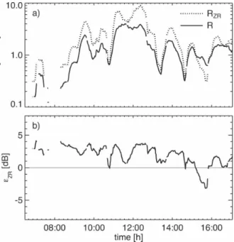
On the other hand, the analysis of the uncertainty associated with theZ–Rtransformation has been car-ried out using 1-min DSD observations for the same events (in Fig. 3 we present the time series ofR,RZR, and ZR, corresponding to the event of 18 October 2000, whereRZRhas been obtained with theZ–R rela-tionship derived from long-term DSD observations in stratiform conditions; see section 5a). These DSDs were measured with the Precipitation Occurrence Sen-sor System (POSS), which is a low-power, continuous-wave, X-band, bistatic, Doppler radar developed by At-mospheric Environment Canada [its technical details
FIG. 1. Locations of the instruments used in this study. The McGill S-band radar is shown as a black triangle (dotted circum-ferences are centered at the radar and separated by 20 km), and the two disdrometers, POSS-1 and POSS-2, were located in down-town Montreal and at Montreal-Trudeau airport, respectively.
TABLE1. Technical characteristics of the McGill S-band radar.
Wavelength 10.4 cm
3-dB beamwidth 0.86°
Rotation speed 6 rotations per minute
Resolution 1 km⫻1°
Elevation angles 24 (0.5°–34°)
can be found in Sheppard (1990) and Sheppard and Joe (1994)]. POSS retrieves the DSD from the average Doppler spectrum, and its big sampling volume (three orders of magnitude larger than a typical disdrometer such as a Joss–Waldvogel model) minimizes undersam-pling problems with a high temporal resolution (Lee and Zawadzki 2005).
In this study, measurements of two different POSS disdrometers have been used: one located in downtown Montreal, 30 km from the McGill radar for the 10 cases prior to 2001, and another one located at Montreal-Pierre Elliott Trudeau International Airport, 15 km from the radar, for the remaining 17 cases.
4. Structure of the range-dependent error
a. Framework of study
The characterization of the range-dependent error has been carried out by simulations as described by Bellon et al. (2005): observations of the 24 elevations of the McGill radar within a sector of 15⫻15 km2
collo-cated with the available POSS have been used as the fine-resolution (reference) 3D field.
Radar observations at further ranges (from 40 to 200 km, every 40 km) have been simulated in a conformal manner by convolving the fine-resolution observations of the reference sector with a Gaussian beam of hori-zontal and vertical widths of 0.86° at half-power
[ap-propriate for the McGill radar; see Bellon et al. (2005) for further details]. From the simulated 3D volume scans at different ranges, 30 polar constant-altitude plan position indicator (CAPPI) maps between 1.3 and 7.1 km (every 0.2 km) have been generated, and the 1.3-km CAPPI for the original sector has been taken as the reference reflectivity field at the ground.
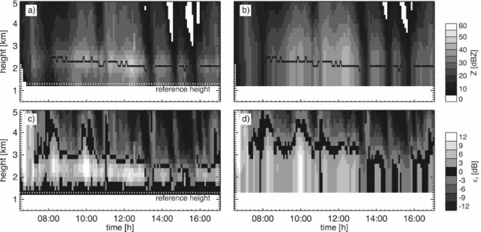
Figure 4 shows one of the cases analyzed in our study: the top panels show time series of radar reflectivity profiles collocated with disdrometer POSS-1 [actually measured VPRs in Fig. 4a, and VPRs simulated at 120 km in Fig. 4b], and the bottom panels show the time series of the resulting range-dependent error when dif-ferent CAPPIs are used to estimate rainfall at the ground. The bright band appears in Fig. 4c as a signif-icant overestimation of the rainfall at the ground (around 2.2 km), while, above, the reflectivity of snow is significantly lower than that observed at the refer-ence height. In Fig. 4b and 4d, the effects of distance can be observed: at 120 km no measurement is obtained below 1.9 km (and, thus, reflectivity is extrapolated from above), and a bigger sampling volume results in vertical gradients of reflectivity that are much smoother than at close range.
Due to the nature of the range-dependent error, and following many authors (Collier 1986; Fabry et al. 1992; Kitchen and Jackson 1993; Koistinen et al. 2003; Bellon et al. 2005), the different statistics from section 2 in FIG. 3. Time series of (a)RandRZR, and (b)ZRobtained from
POSS disdrometer observations measured from 0630 to 1710 UTC 18 Oct 2000. The relationship Z⫽ 237R1.55(derived in
section 5a) has been used to obtainRZR.
FIG. 2. VPR measured at the POSS-1 site at 1159 UTC 18 Oct 2000 (continuous line) and the VPRs simulated from these obser-vations at 80 km (dotted line) and at 160 km (dashed line).
which this error is involved have been estimated as a function of range,r, according to
ˆr共r,h兲⫽ 1 n
兺
i r共r,h,ti兲, 共11兲 ˆr 2共r,h兲⫽1 n兺
i 关r共r,h,ti兲⫺ˆr共r,h兲兴 2, and 共12兲 Cˆr共r,h,⌬t兲⫽ 1 n兺
i 关r共r,h,ti兲⫺ˆr共r,h兲兴⭈关r共r,h,ti ⫹⌬t兲⫺ˆr共r,h兲兴, 共13兲 where ^ indicates that (11)–(13) are estimators of the bias, variance, and covariance, respectively.Additionally, as in Bellon et al. (2005), the results are also shown as a function of the height of the CAPPI used to estimate rain at the ground, h, and stratified according to the height of the brightband peak (see Table 2).
b. Bias and standard deviation of the range-dependent error
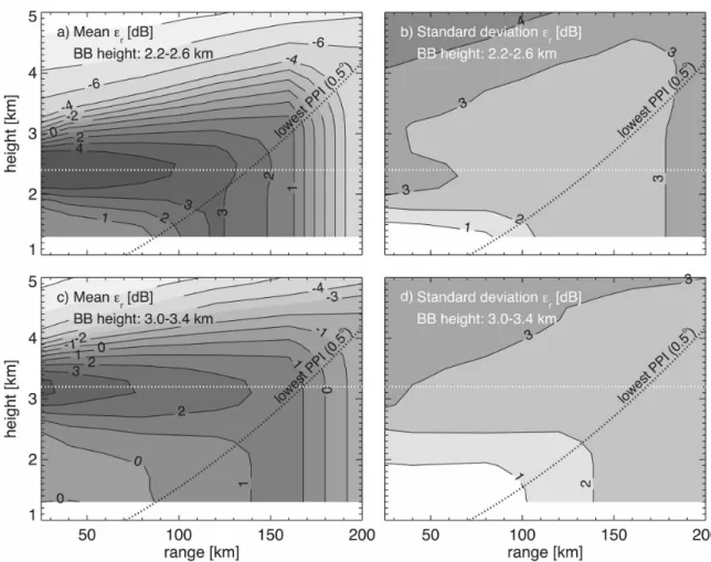
Figure 5 shows the bias and the standard deviation of
r(r,h) obtained from the simulations for those scans where the brightband peak was detected in the ranges 2.2–2.6 and 3.0–3.4 km. Below the melting layer, the bias remains below 1 dB and the standard deviation does not exceed 2 dB. In Fig. 5, the bright band is quite
evident as an overestimation of the reflectivity at the ground (for the presented cases, the mean biases are over 4 dB). Around the bright band, the standard de-viation of the error increases up to 3 dB. This increase in the variability around the brightband peak can be attributed, among other factors, to event-to-event dif-ferences in the role of the main microphysical processes affecting the density of melting snow, which results in significantly different bright bands (Fabry et al. 1992; Fabry and Zawadzki 1995; Huggel et al. 1996; Zawadzki et al. 2005). Above the melting layer, the mean VPR decreases (due to less power backscattered from snow), which results in severe underestimation of the reflectivity measured at the ground. The profiles also show more variability (the standard deviation ofr at close range reaches 4 dB), which can be explained by the following effects: (i) the high variability of the gra-dients of the VPR (which in some cases results in beam overshooting) and the impact of trails in the snow re-gion, and (ii) the variability in the lower part of the VPR with respect to the climatological VPR.
The effects of the range of the observations are threefold: (i) no observations can be obtained below
TABLE2. Distribution of the 171.8 h of data with an identified brightband peak among the six height intervals selected. Height (km) 1.4–1.8 1.8–2.2 2.2–2.6 2.6–3.0 3.0–3.4 ⬎3.4 Duration (h) 9.4 29.5 31.1 33.5 19.3 49.0 FIG. 4. (a) Time series of the McGill S-band radar VPRs collocated with POSS-1 observed from 0630 to 1710 UTC 18 Oct 2000. (b) Time series of VPRs simulated at a range of 120 km for the same period. (c), (d) The corresponding time series of the range-dependent error,r(r,h,t).
the lowest elevation angle and, thus, they have to be extrapolated from elevated heights; (ii) bias profiles at farther ranges are smoother due to the effect of a wider beam (e.g., brightband contamination is lower but ex-tends to higher elevations); and, similarly, (iii) the error variability is slightly lower than the variability at the same height but at closer ranges.
The results presented here are almost identical to those obtained by Bellon et al. (2005) (carried out in Montreal using a very similar simulation method and dataset). There are also some similarities to the results presented by other authors; for example, Kitchen and Blackall (1992) and Koistinen et al. (2003) found long-term biases due to the brightband contamination in low-radar measurements of 1 dB(R) between 50 and 75 km and 2 dB(Z) between 60 and 110 km, and under-estimations at far ranges of ⫺5.6 dB(R) and ⫺8.0 dB(Z) in England and in Finland, respectively. How-ever, the values of the biases due to the bright band can be significantly smoothed due to the fact that no
strati-fication with the height of the brightband peak was taken into account. Kitchen and Blackall (1992) found similar behavior for the standard deviation ofrwith range for observations of the lowest PPI during winter events.
c. Autocorrelation and decorrelation of the range-dependent error
Figure 6 shows the autocorrelation functions (ACF) ofr(r,h) for the height ranges of the brightband peaks shown in the previous section. It can be seen (Figs. 6a and 6b) that when the measurement is in the rain re-gion,r(r,h) decorrelates rapidly (in less than 10 min), indicating that these errors, besides being small (as was shown in the previous section), have no coherent struc-ture, except at far ranges because observations from aloft are extrapolated to construct these low CAPPIs. At higher elevations, where the variances are also higher, stronger correlation is found. In the snow region we note significant differences between the two consid-FIG. 5. Errors in reflectivity at the ground when estimated from reflectivity observed at different ranges and heights for the cases where the brightband peak is (top) between 2.2 and 2.6 km and (bottom) between 3.0 and 3.4 km: (a), (c) bias and (b), (d) standard deviation of the error.
ered classes of bright bands. It is interesting to note that for the cases when the melting layer is between 2.2 and 2.6 km, r(r,h) decorrelates much faster than for the cases with a higher bright band.
Similar results can be seen in Fig. 7, which shows the decorrelation time lags ofr(r,h) (obtained as the time lag for which the correlation falls below 1/e⫽0.37):r decorrelates in less than 15 min in rain measurements, and the maximum correlation appears right below the
melting layer (the decorrelation time goes up to 2.5–4 h) and decays to lower values in the snow.
5. Structure of the uncertainty associated with the
Z–Rtransformation
a. Long-term quantification of the Z–R uncertainty DSD measurements obtained with two POSS located in Montreal were used to characterize the uncertainty FIG. 6. Autocorrelation functions of the range-dependent error when the brightband peak is (left) between 2.2
and 2.6 km at CAPPI heights of (a) 1.3, (c) 1.9, and (e) 3.5 km, and (right) between 3.0 and 3.4 km at CAPPI heights of (b) 1.5, (d) 3.1, and (f) 4.1 km.
in theZ–Rtransformation when a singleZ–R relation-ship is used to estimate rainfall from reflectivity obser-vations.
Here, from 1-min DSD observations corresponding to the events described in sections 3 and 4,R(mm h⫺1) andZ(mm6m⫺3) were computed using
R⫽6 ⭈10⫺4
冕
Dmin Dmax D3共D兲N共D兲dD and 共14兲 Z⫽冕
Dmin Dmax D6N共D兲dD, 共15兲whereDis the diameter (mm),(D) the velocity (m s⫺1),
andN(D) is the concentration of drops of diameterD (mm⫺1m⫺3).
DSD observations have been averaged over a 20-min window to ensure that the DSD variability in disdro-metric observations is equivalent to the variability in the 15⫻15 km2 resolution of radar observations. We
chose 20 min because it is the time interval that leads to the best correlation between POSS and radar reflectiv-ity averaged over a 15⫻15 km2sector (see an example
in Fig. 8).
TheZ–R scatterplot obtained from disdrometer ob-servations of the 27 analyzed events is presented in Fig. 9 (the dashed line represents the best fit; Z⫽237R1.55).
ThisZ–Rrelationship is very similar to the climatologi-cal Z–R relationship derived by Lee and Zawadzki (2005) for Montreal (Z⫽210R1.47) and to the widely used Z ⫽ 200R1.6 obtained by Marshall and Palmer (1948).
By construction, no long-term bias is expected in rainfall estimated from reflectivity observations. How-ever, the variability in the DSD [both from storm to
storm and within a single storm, as discussed by Lee and Zawadzki (2005)] results in significant scatter in the R–RZR plot (as shown in Fig. 9). In a climatological sense, all scatter must be considered as random error of individual 20-min observations, although an important bias and a reduced random error are present on a storm-by-storm basis. For the analyzed dataset, the “cli-matological” standard deviation ofZR, obtained with an equation analogous to (12), resulted inˆZR⫽1.37 dB(R).
Lee and Zawadzki (2005) also quantified the vari-ability of theZ–Rrelationships at different scales using long-term observations collected with the same instru-ments, but for a different set of events, including some convective storms. For an averaging window of 20 min and using the climatological Z–R relationship, they found similar values for the standard deviation of the error in linear units (1.4 mm h⫺1) and for the random
FIG. 8. Time series of the reflectivity computed from POSS DSD observations (dotted line) and observed with the McGill S-band radar 1300 m over the POSS (continuous line) from 0630 to 1710 UTC 18 Oct 2000.
FIG. 7. Decorrelation time (h) of the range-dependent error when the reflectivity at the ground is estimated from elevated reflectivity measurements at different ranges when the brightband peak is between (left) 2.2 and 2.6, and (right) 3.0 and 3.4 km.
component (44%; with our dataset, 1.7 mm h⫺1 and 35%, respectively).
b. Autocorrelation and decorrelation ofZR
Lee et al. (2007) proposed a two-component model to characterize the structure of ZR: a broken-line model to characterize the large-scale variability and a power law model for the Fourier spectrum at storm scale, since they found scaling properties in small-scale fluctuations ofZR.
Assuming their model, Fig. 10 shows the sample ACF and the second-order structure function of the residuals
ZRfor the analyzed dataset using (13). The decorrela-tion time of around 130 min is significantly longer as compared to the 60 min for the cases analyzed by Lee et al. (2007). This is evidence of the effects of the coarser resolution of the observations analyzed here on the shape of the error covariance matrix (further dis-cussion is presented in section 8).
6. Cross correlation betweenr andZR
As discussed above, besides the individual contri-butions of the two analyzed sources of error, the ex-pression for the error covariance of the error also in-cludes the cross term involvingrandZR[cov{r(x1,h),
ZR(x2,h0)} in (10)].
In this section we analyze the cross correlation be-tween the time series ofr(r,h,t), as estimated from the
radar reflectivity profiles used in section 4, and the col-locatedZR(t) obtained from POSS observations. For this, it is necessary to have a well-calibrated radar. In our case, the calibration of the McGill S-band radar is regularly monitored using POSS measurements (Lee and Zawadzki 2006) and, thus, the agreement in the reflectivity measurements of the two instruments is rea-sonable, as can be appreciated in the example of Fig. 8. The sample cross correlation between the time series of the range-dependent error,r(r,h,t), and the error
due to the Z–R variability, ZR(t), has been calcu-lated as ˆr⫺ZR共r,h,⌬t兲⫽ 1 ˆrˆZR
冋
1 n兺
i 兵关r共r,h,ti兲 ⫺ˆr共r,h兲兴⭈ ZR共ti⫹⌬t兲其册
. 共16兲 The estimated ˆr⫺ZR(r, h,⌬t) corresponding to the example of Figs. 3 and 4 is presented in Fig. 11. It can be appreciated that correlations stay low in the rain region and at higher elevations (over 3 km), and there is a significant maximum of correlation around the mean height of the brightband peak. Thus, there is cor-relation betweenZRat the ground and the extrapola-tion error around the brightband peak, r(r, hpeak).Assuming a uniform VPR below the bright band,
r(r,hpeak) would be a proxy for the brightband
inten-sity,⌬Zpeak-to-rain [defined as the difference in dB
be-tween the reflectivity of the brightband peak and the reflectivity of the rain right below the bright band, as in Klaassen (1988) or Fabry and Zawadzki (1995)]. Thus, FIG. 9. AZ–Rscatterplot obtained from the DSD POSS
mea-surements corresponding to the entire dataset analyzed in this study. Each dot corresponds to a 1-min observation averaged over a window of 20 min. The dashed gray line represents the best fit to the observations (Z⫽237R1.55).
FIG. 10. Structure function (black line) and ACF (gray line) of
the residuals of theZ–Rtransformation,ZR, computed from the
our results confirm the direct relationship between the brightband intensity and the localZ–Rrelationship, in-dicating that the main physical processes involved in the growth of snow determine both the characteristics of the bright band (in this case,⌬Zpeak-to-rain), as
dis-cussed in Fabry and Zawadzki (1995) and quantita-tively evaluated in Zawadzki et al. (2005), and the re-sultingZ–Rrelationship at the ground (Zawadzki and Lee 2004; Bellon et al. 2007), here, expressed as the departuresZRfrom the long-termZ–Rrelationship.
Huggel et al. (1996), following the results of Wald-vogel (1974) and WaldWald-vogel et al. (1993), found a very
tweenr(r0,h) andZRobtained from the dataset of 27 events, where the height is now relative to the height of the brightband peak, and the lag needed by brightband melting particles to reach the ground, ⌬tpeak-to-ground,
has been subtracted from the time lag. Figure 12 shows similar behavior to the example case shown in Fig. 11: low correlation between r(r0, h) and ZR below the bright band and above the melting layer, as well as a significant maximum in the vicinity of the bright band. Results appear smoother when the same figure has been derived using VPRs simulated at 120 km, due to the effect of a wider beam (Fig. 13b), which extends the effects of the correlation betweenrwhen observations are extrapolated from the brightband peak andZR. 7. Resulting error covariance
From the results shown in previous sections, the co-variance of(r,h,t)⫽(1/b)r(r,h,t)⫹ ZR(t) can be estimated using (10).
FIG. 12. Median cross correlation between the times series ofr(r0,h) andZR, corresponding to the 27 events
analyzed in this study, where the height has been referred to the height of the brightband peak and the time needed for melting particles to reach the ground has been subtracted from the lag. (a) Results using observations from the McGill S-band radar at the POSS sites and (b) those using reflectivity simulations corresponding to a range of 120 km.
FIG. 11. Cross correlation between the time series ofr(r0,h)
andZRobtained from the series of Figs. 3, 4a, and 4c, from radar
and POSS-1 observations measured from 0630 to 1710 UTC 18 Oct 2000.
Figures 13 and 14 show the resulting error ACF and covariance, respectively, at close range and at 120 km for the cases when the brightband peak is located be-tween 2.2 and 2.6 km and 3.0 and 3.4 km. The errors,, below the melting layer have longer decorrelation lags than above. This is due to the fact that in the lower heights the error is dominantly due to theZ–R trans-formation. Therefore, below the melting layer,ˆ(r,h) stays between 1.4 and 2 dB(R), and the decorrelation lags between 1.5 and 2 h (very similar to the decorre-lation lags ofZR). For elevated observations, the stan-dard deviation of the error is around 2.5–3.5 dB(R) and the decorrelation is significantly shorter (between 40 and 60 min). This is due to the fact that, in this region,
ˆ(r, h) is significantly higher than ˆZR (as shown in previous sections), and, therefore, the error with range has more weight in the resulting ACF. Similarly, at fur-ther ranges, the error decorrelation is around 1 h, though the ACF and the covariance are smoother with height due to the effect of a wider beam.
Up to this point we have only considered the
tempo-ral structure of the error affecting radar rainfall esti-mates. Similarly to Zawadzki (1973) and Lee et al. (2007), here we assume the validity of the Taylor hy-pothesis to infer the spatial structure of this error. As-suming the climatological advection velocity of precipi-tation patterns for the region of Montreal (around 40 km h⫺1), the spatial decorrelation of the error affecting radar rainfall estimates,, becomes around 60–80 km at near range and low heights, and decreases up to 40 km when the observations are taken aloft.
8. Conclusions and discussion
In this study we have developed a methodology for the analysis of the error covariance matrix of radar rainfall estimates at the ground. Our approach is based on detailed study of each source of error so that it can be applied to different conditions, regional characteris-tics, and radar operations. This method also provides a physical understanding of error sources affecting radar measurements.
FIG. 13. ACF of(r,h) obtained for the cases where the brightband peak is (a), (b) between 2.2 and 2.6 km and (c), (d) 3.0 and 3.4 km. Results from using (left) radar observations at the POSS sites and (right) reflectivity simulations at 120 km from the radar. The white line corresponds to ACF values of 1/e.
Our aim is to give a better characterization of errors for the assimilation of surface radar rainfall observa-tions into NWP mesoscale models. We have concen-trated here on the structure of the errors resulting from the two major sources of uncertainty affecting radar rainfall observations at nonattenuated wavelengths (i.e., the range-dependent error and the error associ-ated with theZ–R transformation) and only in strati-form conditions. For this purpose we analyzed long time series of collocated radar reflectivity and DSD observations obtained in Montreal.
The analysis of the biases introduced by the range-dependent error has shown characteristics already found by other authors: little bias close to the ground (below the bright band), a significant overestimation when reflectivity observations at the ground are extrap-olated from the melting layer, and progressive under-estimation as the radar samples at higher elevations. The effects of the beamwidth increasing with range can be appreciated as a clear smoothing of radar observa-tions. The autocorrelation function of these errors has
also been characterized and we show that the errors are mainly uncorrelated in the rain region. As the observa-tions are taken farther aloft, the errors become more correlated (with decorrelation lags below the bright-band peak around 2 h) and slightly less correlated in the snow region. The latter is somewhat surprising because one would expect more correlation in snow due to the more uniform nature of the fields and could be attrib-uted to the small-scale variability of the VPRs in the snow region.
The errors due to the uncertainty associated with the reflectivity transformation at the ground when a single Z–Rrelationship is used have also been characterized in terms of their variability and average ACF. During stratiform conditions, a standard deviation of 1.37 dB has been found and the decorrelation time shows that the consistency of the departures from the climatologi-cal Z–R persists for around 2 h for resolutions corre-sponding to 15⫻15 km2.
Finally, we have also studied the cross correlation between the two analyzed sources of error. We have FIG. 14. Covariance [dB(R)2] of(r,h) obtained for the cases where the brightband peak is (a), (b) between 2.2
and 2.6 km and (c), (d) between 3.0 and 3.4 km. (left) Results using radar observations at the POSS sites and (right) from using reflectivity simulations at 120 km from the radar.
shown that, below and above the melting layer, negli-gible correlation exists between the two types of errors while contamination by bright band is responsible for a significant correlation. This simply reflects the fact that the physical processes dominating the generation of precipitation above the melting layer have a direct ef-fect on both the intensity of the bright band (for which the error with range is a proxy) and on the resulting Z–Rrelationship at the ground.
The resulting error covariance shows that the stan-dard deviation of the resulting error remains within very narrow limits at near ranges and at low heights [between 1.5 and 2 dB(R)], while the ACF shows that decorrelates at lags of 1.5–2 h or, alternatively, 60–80 km. At farther ranges, when the observations are ob-tained in the melting layer or aloft, the standard devia-tion of increases up to 2.5–3.5 dB(R) and the error decorrelates faster (after 40–60 min, or 25–40 km).
Considering the results described above and that, with the resolution of the observations used in this pa-per (15⫻15km2), the obtained decorrelation distances
of 60–80 km result in four to six grid points (or two to three grid points for elevated observations), we con-clude that (i) the usual hypothesis of homogenous er-rors is not realistic at ranges where the CAPPI used to estimate rainfall at the ground is constructed from the lowest PPI (i.e., from observations significantly higher than the nominal CAPPI height), and (ii) at the region where remains within reasonable limits (where the radar measures in the rain region), the decorrelation distance of the error is significantly longer than the resolution of the observations and, therefore, the as-sumption of uncorrelated errors (very common in schemes assimilating radar rainfall measurements) is not generally valid.
From a more hydrological perspective, Ciach et al. (2007) and GBSTZ looked into the problem by char-acterizing the structure of the residuals between radar rainfall estimates at ground and gauge observations. In this way, they account for the general effects of the errors affecting radar estimates, assuming the gauges to be perfect.
The approach to computing radar errors used here has more similarities to that of Jordan et al. (2003). The main differences are (i) we used a much longer dataset and (ii) in their study, the analyzed error sources were assumed to be independent (which, as has been shown, is not necessarily satisfied when the measurements are contaminated by the bright band) and stationary in space.
In our approach, there are some assumptions and considerations that need further discussion and that could be taken into account in further characterizations
of the error covariance matrix of radar rainfall esti-mates:
(i) Both radar rainfall estimates and the error have been considered in logarithmic units. By doing this, we assume that the distribution of the error
(x) is more Gaussian-like than the multiplicative version of the error [as was also argued by Jordan et al. (2003) and Ciach et al. (2007)]. This has been adopted so as to satisfy the hypothesis of Gaussian errors implicit in most of the assimilation schemes; however, at the same time, it also imposes assimi-lating rainfall observations in logarithmic units. (ii) We have neglected here to consider a possible
de-pendence of the error structure on rainfall inten-sity [as was also done by Jordan et al. (2003) and GBSTZ]. However, since here we limit our study to stratiform rain, and consequently to a limited dynamic range of intensities, we should expect little advantage in further stratification with inten-sity, although this remains to be verified.
(iii) The presented methodology assumes that the height of the brightband peak is known, and this is not always the case within the framework of radar data assimilation. Here, we propose using the in-formation of the 0°C isotherm provided by the background term and/or the information about the brightband peaks identified by an algorithm such as the one proposed by Sanchez-Diezma et al. (2000).
(iv) The fact that the study has been carried out using long-term observations means that the resulting error covariance matrix is representative of the mean stratiform conditions and it may be not fully appropriate for each individual situation. It also has to be mentioned that it is limited to certain conditions of the quality control of the data. Mainly, it is valid when no correction is applied to compensate for the range-dependent error [or, al-ternatively, when the climatological VPRs strati-fied according to the height of the brightband peak are used to compensate the range-dependent er-ror, similar to methodology C3 of Bellon et al. (2007); we would expect less correlated r if method C2 in the same paper were applied] and when a climatological Z–R transformation for stratiform precipitation is used. Finally, it has to be mentioned that although the methodology can be applied elsewhere, the results shown here corre-spond to the specific region where the study has been done (Montreal, Quebec, Canada) and to the scanning strategy and characteristics of the radar used for the analysis. For instance, characterizing
and it is, thus, not correct to use the results pre-sented in this work for different resolutions (in a follow-up paper, we will discuss the impact of reso-lution on the resulting error structure).
(vi) In our study we have only characterized the instru-mental error of radar rainfall estimates, while the error covariance matrix of observationsR should also include the component due to the uncertain-ties in the observation operatorH( ) used to trans-form model variables to the observation domain (see Kalnay 2003). The error covariance matrix derived in our study would, thus, underestimate the errors affecting the assimilation of radar rain-fall estimates into NWP models.
It is also worth mentioning that one interesting ap-plication of the error covariance matrix of radar rainfall estimates (as the one proposed here) is to study how the uncertainty in rainfall observations is propagated through a rainfall–runoff model in terms of the uncer-tainty in simulated flows (see Krzysztofowicz 1998; Krzysztofowicz 2002). In this sense, some authors (e.g., Jordan et al. 2003; Berenguer et al. 2005; Germann et al. 2006; Ciach et al. 2007) propose a probabilistic ap-proach based on ensemble of equiprobable rainfall fields compatible with radar observations [first at-tempts have been presented in the works of Pierce et al. (2005), Lee et al. (2007), Berenguer et al. (2006), and GBSTZ] and use them as inputs for a rainfall–runoff model to analyze the impact of the uncertainty in rain-fall products in terms of the simulated discharges.
Acknowledgments.This work is part of the Canadian Weather Research Program and was made possible by the support of Environment Canada given to the J. S. Marshall Radar Observatory. Thanks are due to Dr. Aldo Bellon, who reviewed a preliminary version of the paper, and to Dr. Luc Fillion, for useful discussions on the need to improve the characterization of the error
998–1015.
——, ——, A. Kilambi, and I. Zawadzki, 2007: Real-time com-parisons of VPR-corrected daily rainfall estimates with a gauge mesonet.J. Appl. Meteor. Climatol.,46,726–741. Berenguer, M., C. Corral, R. Sanchez-Diezma, and D.
Sempere-Torres, 2005: Hydrological validation of a radar-based now-casting technique.J. Hydrometeor.,6,532–549.
——, D. Sempere-Torres, R. Sanchez-Diezma, G. Pegram, I. Zawadzki, and A. Seed, 2006: Modelization of the uncer-tainty associated to radar-based nowcasting techniques. Im-pact in flow simulation.Proc. Fourth European Conf. on Ra-dar in Meteorology and Hydrology (ERAD), Barcelona, Spain, Group of Applied Research on Hydrometeorology– Universitat Politècnica de Catalunya (GRAHI–UPC), 575– 578.
Caya, A., J. Sun, and C. Snyder, 2005: A comparison between the 4DVAR and the ensemble Kalman filter techniques for radar data assimilation.Mon. Wea. Rev.,133,3081–3094. Chung, K.-S., I. Zawadzki, M. K. Yau, and L. Fillion, 2007:
Ini-tialization of midlatitude convective storms by assimilation of single Doppler radar observations. Preprints,33rd Int. Conf. on Radar Meteorology, Cairns, Australia, Amer. Meteor. Soc., P5.5. [Available online at http://ams.confex.com/ams/ pdfpapers/122990.pdf.]
Ciach, G. J., and W. F. Krajewski, 1999: On the estimation of radar rainfall error variance.Adv. Water Res.,22,585–595. ——, ——, and G. Villarini, 2007: Product-error-driven
uncer-tainty model for probabilistic quantitative precipitation esti-mation with NEXRAD data.J. Hydrometeor.,8,1325–1347. Collier, C., 1986: Accuracy of rainfall estimates by radar, Part I: Calibration by telemetering raingauges.J. Hydrol.,83,207– 223.
Crook, N. A., and J. Z. Sun, 2002: Assimilating radar, surface, and profiler data for the Sydney 2000 Forecast Demonstration Project.J. Atmos. Oceanic Technol.,19,888–898.
Daley, R., 1991:Atmospheric Data Analysis. Cambridge Univer-sity Press, 471 pp.
Deblonde, G., J. F. Mahfouf, and B. Bilodeau, 2007: One-dimensional variational data assimilation of SSM/I observa-tions in rainy atmospheres at MSC.Mon. Wea. Rev., 135,
152–172.
Errico, R. M., L. Fillion, D. Nychka, and Z. Q. Lu, 2000: Some statistical considerations associated with the data assimilation of precipitation observations.Quart. J. Roy. Meteor. Soc.,
126,339–359.
the melting layer of precipitation and their interpretation.J. Atmos. Sci.,52,838–851.
——, G. L. Austin, and D. Tees, 1992: The accuracy of rainfall estimates by radar as a function of range. Quart. J. Roy. Meteor. Soc.,118,435–453.
Fillion, L., and R. Errico, 1997: Variational assimilation of pre-cipitation data using moist convective parameterization schemes: A 1DVAR study.Mon. Wea. Rev.,125,2917–2942. Germann, U., and J. Joss, 2002: Mesobeta profiles to extrapolate radar precipitation measurements above the Alps to the ground level.J. Appl. Meteor.,41,542–557.
——, M. Berenguer, D. Sempere-Torres, and G. Salvadè, 2006: Ensemble radar precipitation estimation—A new topic on the radar horizon.Proc. Fourth European Conf. on Radar in Meteorology and Hydrology (ERAD),Barcelona, Spain, Group of Applied Research on Hydrometeorology–Universitat Politècnica de Catalunya (GRAHI–UPC), 559–562. Guo, Y. R., Y. H. Kuo, J. Dudhia, D. Parsons, and C. Rocken,
2000: Four-dimensional variational data assimilation of het-erogeneous mesoscale observations for a strong convective case.Mon. Wea. Rev.,128,619–643.
Hu, M., and M. Xue, 2007: Impact of configurations of rapid intermittent assimilation of WSR-88D radar data for the 8 May 2003 Oklahoma City tornadic thunderstorm case.Mon. Wea. Rev.,135,507–525.
Huggel, A., W. Schmid, and A. Waldvogel, 1996: Raindrop size distributions and the radar bright band.J. Appl. Meteor.,35,
1688–1701.
Jordan, P. W., A. W. Seed, and P. E. Weinmann, 2003: A stochas-tic model of radar measurement error in rainfall accumula-tions at catchment scale.J. Hydrometeor.,4,841–855. Joss, J., and A. Waldvogel, 1990: Precipitation measurement and
hydrology.Radar in Meteorology,D. Atlas, Ed., Amer. Me-teor. Soc., 577–606.
Kalnay, E., 2003:Atmospheric Modeling, Data Assimilation and Predictability. Cambridge University Press, 341 pp. Kitchen, M., and R. M. Blackall, 1992: Representativeness errors
in comparisons between radar and gauge measurements of rainfall.J. Hydrol.,134,13–33.
——, and P. M. Jackson, 1993: Weather radar performance at long range—Simulated and observed. J. Appl. Meteor.,32,975– 985.
Klaassen, W., 1988: Radar observations and simulation of the melting layer of precipitation.J. Atmos. Sci.,45,3741–3753. Koistinen, J., D. B. Michelson, H. Hohti, and M. Peura, 2003: Operational measurement of precipitation in cold climates.
Weather Radar—Principles and Advanced Applications, P. Meishcner, Ed., Springer, 78–114.
Krzysztofowicz, R., 1998: Probabilistic hydrometeorological fore-casts: Toward a new era in operational forecasting. Bull. Amer. Meteor. Soc.,79,243–251.
——, 2002: Probabilistic flood forecast: Bounds and approxima-tions.J. Hydrol.,268,41–55.
Lee, G. W., and I. Zawadzki, 2005: Variability of drop size distri-butions: Time-scale dependence of the variability and its ef-fects on rain estimation.J. Appl. Meteor.,44,241–255. ——, and ——, 2006: Radar calibration by gage, disdrometer, and
polarimetry: Theoretical limit caused by the variability of drop size distribution and application to fast scanning opera-tional radar data.J. Hydrol.,328,83–97.
——, A. Seed, and I. Zawadzki, 2007: Modeling the variability of drop size distributions in space and time.J. Appl. Meteor. Climatol.,46,742–756.
MacPherson, B., 2001: Operational experience with assimilation of rainfall data in the Met Office mesoscale model.Meteor. Atmos. Phys.,76,3–8.
——, and Coauthors, 2003: Assimilation of radar data in numeri-cal weather predicition (NWP) models.Weather Radar— Principles and Advanced Applications,P. Meischner, Ed., Springer, 78–114.
Marecal, V., and J. F. Mahfouf, 2000: Variational retrieval of tem-perature and humidity profiles from TRMM precipitation data.Mon. Wea. Rev.,128,3853–3866.
Marshall, J. S., and W. M. Palmer, 1948: The distribution of rain-drops with size.J. Meteor.,5,165–166.
Mittermaier, M., R. J. Hogan, and A. Illingworth, 2004: Using mesoscale winds for correcting wind-drift errors in radar es-timates of surface rainfall.Quart. J. Roy. Meteor. Soc.,130,
2105–2123.
Montmerle, T., A. Caya, and I. Zawadzki, 2001: Simulation of a midlatitude convective storm initialized with bistatic Doppler radar data.Mon. Wea. Rev.,129,1949–1967.
Pierce, C., N. Bowler, A. W. Seed, A. Jones, D. Jones, and R. Moore, 2005: Use of a stochastic precipitation nowcast scheme for fluvial flood forecasting and warning.Atmos. Sci. Lett.,6,78–83.
Richards, W. G., and C. L. Crozier, 1983: Precipitation measure-ment with a C-band weather radar in southern Ontario. At-mos.–Ocean,21,125–137.
Sanchez-Diezma, R., I. Zawadzki, and D. Sempere-Torres, 2000: Identification of the bright band through the analysis of volu-metric radar data.J. Geophys. Res.,105,2225–2236. Sheppard, B. E., 1990: Measurement of raindrop size distributions
using a small Doppler radar.J. Atmos. Oceanic Technol.,7,
255–268.
——, and P. I. Joe, 1994: Comparison of raindrop size distribution measurements by a Joss–Waldvogel disdrometer, a PMS 2DG spectrometer, and a POSS Doppler radar.J. Atmos. Oceanic Technol.,11,874–887.
Smith, J. A., and W. F. Krajewski, 1993: A modeling study of rainfall rate reflectivity relationships.Water Resour. Res.,29,
2505–2514.
Sun, J., 2005a: Convective-scale assimilation of radar data: Prog-ress and challenges.Quart. J. Roy. Meteor. Soc.,131,3439– 3463.
——, 2005b: Initialization and numerical forecasting of a supercell storm observed during STEPS.Mon. Wea. Rev.,133,793– 813.
——, and N. A. Crook, 1997: Dynamical and microphysical re-trieval from Doppler radar observations using a cloud model and its adjoint. Part I: Model development and simulated data experiments.J. Atmos. Sci.,54,1642–1661.
——, and J. W. Wilson, 2003: The assimilation of radar data for weather prediction.Radar and Atmospheric Science: A Col-lection of Essays in Honor of David Atlas, Meteor. Monogr.,
No. 52, Amer. Meteor. Soc., 175–198.
Vignal, B., H. Andrieu, and J. D. Creutin, 1999: Identification of vertical profiles of reflectivity from volume scan radar data.J. Appl. Meteor.,38,1214–1228.
Waldvogel, A., 1974: TheN0jump of raindrop spectra.J. Atmos.
Sci.,31,1067–1078.
——, W. Henrich, and L. Mosimann, 1993: New insight into the coupling between snow spectra and raindrop size distribu-tions. Preprints,26th Conf. on Radar Meteorology,Norman, OK, Amer. Meteor. Soc., 602–604.