Worcester Polytechnic Institute
Digital WPI
Masters Theses (All Theses, All Years)
Electronic Theses and Dissertations
2012-04-30
A Graph Theoretic Clustering Algorithm based on
the Regularity Lemma and Strategies to Exploit
Clustering for Prediction
Shubhendu Trivedi
Worcester Polytechnic Institute
Follow this and additional works at:
https://digitalcommons.wpi.edu/etd-theses
This thesis is brought to you for free and open access byDigital WPI. It has been accepted for inclusion in Masters Theses (All Theses, All Years) by an authorized administrator of Digital WPI. For more information, please [email protected].
Repository Citation
Trivedi, Shubhendu, "A Graph Theoretic Clustering Algorithm based on the Regularity Lemma and Strategies to Exploit Clustering for Prediction" (2012).Masters Theses (All Theses, All Years). 573.
A Graph-Theoretic Clustering Algorithm based on
the Regularity Lemma and Strategies to Exploit
Clustering for Prediction
Shubhendu Trivedi
Submitted in partial fulfillment of the requirements for the degree
of Master of Science
in the Department of Computer Science
Worcester Polytechnic Institute
2012
Thesis Approved:
Dr. Neil T. Heffernan (Thesis Advisor)
Dr. G´abor N. S´ark¨ozy (Thesis Advisor)
Dr. Sonia Chernova (Thesis Reader)
The mind can be highly delighted in two ways: by perception and conception. But the former demands a worthy object, which is not always at hand, and a proportionate culture, which one does not immediately attain. Conception, on the other hand, requires only susceptibility: it brings its subject-matter with it, and is itself the instrument of culture.
Acknowledgments
I would like to express my deepest gratitude for all who have been directly or indirectly responsible for this work. To start with I would like to thank my great advisers: Professor Neil Heffernan and Professor G´abor S´ark¨ozy for their constant support and encouragement. Professor Heffernan has had a big hand by indirectly moulding what I worked on by con-taining my overtly enthusiastic disposition so that it could be channelled into something more useful and productive. Professor S´ark¨ozy for the wise words and the constant coun-selling about research and life in general. Thanks to my Thesis Reader Professor Sonia Chernova for being so prompt and helpful. A very special thanks to Prof. Glynis Hamel for her help in getting me subjects that I could manage to TA for and all the Professors that I assisted in some course (Prof. Joshua Guttman, Prof. S´ark¨ozy, Prof. Hugh Lauer and Prof. Heffernan). I am also thankful to Prof. Hugh Lauer for his kind words of encouragement about my work and not to mention - making the experience of TAing for a Systems course (and yet maintaining the tempo for research) so enjoyable. Thanks to Zach Pardos for the innumerable conversations about work and persevering with my countless digressions. I am also grateful to Fei Song for many insightful discussions on some of this work and for his both direct and indirect help in improving my understanding of many ideas. I am also grateful to Professor Stanley Selkow for many sharp insights and meetings that often changed my way of looking at things. Thanks to Professor Carolina Ruiz for her support in harder times.
A special thanks to Mike Voorhis and John Leveillee for always being there with help for both my research computing issues and those with courses that I was assigned to assist. I am also grateful to Diane Baxter for her help in getting a lot of paper work done quickly and making it fun. I am also grateful to all the other faculty members in the CS Department for making the experience and the time that went into this work so much fun. Thanks to
my room-mates Adinath and Tanmay for putting up with my weird work schedules and sleeping hours.
Further afield I would like to thank my school physics teacher Mrs Bhawana Danak for discussing some issues back in high school that got me interested in spectral stuff to start with.
Lastly, but more importantly, thanks to my parents, my brother and sister and all my friends for their constant love and support. Finally, I would like express my deepest gratitude to Ritika, without whom none of this could have been possible.
ABSTRACT
The fact that clustering is perhaps the most used technique for exploratory data analysis is only a semaphore that underlines its fundamental importance. The general problem state-ment that broadly describes clustering as the identification and classification of patterns into coherent groups also implicitly indicates it’s utility in other tasks such as supervised learning. In the past decade and a half there have been two developments that have altered the landscape of research in clustering: One is improved results by the increased use of graph theoretic techniques such as spectral clustering and the other is the study of clustering with respect to its relevance in semi-supervised learning i.e. using unlabeled data for improving prediction accuracies. In this work an attempt is made to make contributions to both these aspects. Thus our contributions are two-fold: First, we identify some general issues with the spectral clustering framework and while working towards a solution, we introduce a new algorithm which we call “Regularity Clustering” which makes an attempt to harness the power of the Szemer´edi Regularity Lemma, a remarkable result from extremal graph theory for the task of clustering. Secondly, we investigate some practical and useful strategies for using clustering unlabeled data in boosting prediction accuracy. For all of these contribu-tions we evaluate our methods against existing ones and also apply these ideas in a number of settings.
Table of Contents
Introduction 1
0.1 Contributions and Overview . . . 2
I Preliminaries 5 1 Preliminaries 6 1.1 Clustering . . . 6
1.2 Spectral Clustering . . . 7
1.2.1 Self-Tuning Spectral Clustering . . . 12
II Regularity Clustering 14 2 Motivation to Regularity Clustering 15 2.1 Introduction . . . 15
2.2 Clustering . . . 17
2.3 Prior Attempts to Use the Regularity Lemma for Practical Applications . . 18
3 The Szemer´edi Regularity Lemma 20 3.1 Definitions and Notation . . . 20
3.2 Original Statement . . . 22
3.3 Algorithmic Versions of the Regularity Lemma . . . 22
3.3.1 Alon-Duke-Lefmann-R¨odl-Yuster Version . . . 22
3.3.2 Frieze-Kannan Version . . . 26
3.4 Using the Regularity Lemma . . . 27
4 Regularity Clustering 28 4.1 Modifications to the Constructive Version . . . 28
4.2 A Two Phase Strategy for Clustering . . . 30
4.3 Empirical Validation . . . 31
4.3.1 Datasets and Metrics Used . . . 31
4.3.2 Case Study . . . 33
4.3.3 Clustering Results on Benchmark Datasets . . . 39
4.4 Discussion and Future Directions . . . 40
III Clustering for Prediction 44 5 Clustering for Prediction 45 5.1 PAC-MDL Bounds and Clustering as Classification . . . 46
5.2 A Simple Bagging Strategy . . . 48
5.2.1 k as a Tunable Parameter . . . 50
5.3 Combining Predictions . . . 51
5.3.1 An Information Theoretic View of Clustering . . . 52
5.3.2 Ensemble Learning . . . 53
5.3.3 Methodology for Combining Predictions . . . 54
5.4 Similarity with Existing Methods . . . 54
5.5 Empirical Validation . . . 55 5.5.1 Algorithms . . . 55 5.5.2 Datasets . . . 56 5.5.3 Methodology . . . 57 5.5.4 Results . . . 59 5.6 Future Work . . . 67
6 Improving Student Test Score Prediction 70 6.1 Motivation and Literature Survey . . . 70
6.2 Data and Metrics . . . 72
6.3 Methodology . . . 73
6.4 Results using k-means Clustering . . . 74
6.5 Results Using Spectral Clustering . . . 75
6.6 Contributions and Future Work . . . 77
7 Improving Knowledge Tracing 80 7.1 Motivation and Background on Knowledge Tracing . . . 80
7.1.1 Bayesian Knowledge Tracing . . . 82
7.2 Clustered Knowledge Tracing . . . 83
7.3 Empirical Validation . . . 84
7.3.1 Datasets . . . 84
7.3.2 Results . . . 85
7.4 Discussion . . . 87
8 Co-Clustering for Prediction 89 8.1 Why Co-Cluster? . . . 90
8.2 Co-Clustering . . . 92
8.2.1 Notation and Definitions . . . 92
8.2.2 Spectral Co-Clustering . . . 94
8.3 Co-Clustering for Bootstrapping . . . 97
8.3.1 Blending Predictions . . . 98
8.4 Experimental Validation . . . 98
8.4.1 Dataset Description and Context . . . 99
8.4.2 Experimental Results . . . 101
8.5 Discussion and Future Work . . . 102
IV Concluding Remarks 105 9 Conclusions 106 9.1 Future Work . . . 107
V Bibliography 110
Bibliography 111
List of Figures
1.1 Results of using k-means on two synthetic datasets. . . 9
1.2 Results of using Spectral Clustering on a synthetic dataset. . . 12 4.1 A Two Phase Strategy for Clustering . . . 31
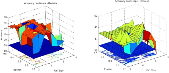
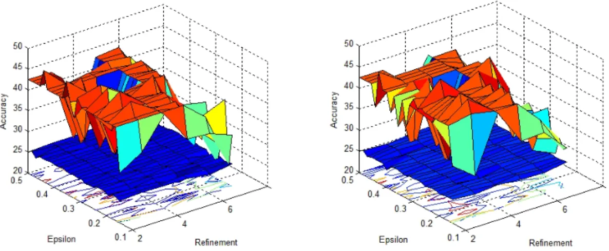
4.2 Accuracy Landscape for Regularity Clustering on the Red Wine Dataset for
different values ofεand refinement sizel(with k = 6 on the left and k = 3 on the right). The Plane cutting through in blue represents accuracy by running self-tuned spectral clustering using the fully connected similarity graph. . . 35 4.3 Accuracy Landscape on the Red Wine Dataset (with k = 6 on the left and k =
3 on the right) when the most irregular pair is considered in each refinement. The Plane cutting through in blue represents accuracy by running self-tuned spectral clustering using the fully connected similarity graph. . . 38 5.1 A “Prediction Model”. A “Prediction Model” is composed of k cluster models
(P Mk). It should be noted that any other method for regression could be
used in place of Linear Regression . . . 49 5.2 Mapping a test point to a cluster to make a prediction on it . . . 50
5.3 Generation of multiple prediction models by using k as a free parameter.
Each of these prediction models will make a prediction on the test set. These predictions can then be combined together by a nave ensemble to get a final prediction. . . 51
5.4 The error profiles for all 11 datasets for stepwise linear regression. The x-axis represents the number of prediction models averaged from 1. The bar marked in red indicates the one that has been chosen by the first heuristic as the final prediction. In many cases we notice that this is clearly a sub-optimal choice. The chosen value and the lowest value in the error profile for each dataset should be contrasted with the value of CVk mentioned in the table. Since the number of prediction models to average chosen is different in each fold
by the second method, it has not been represented in the graph. . . 62
5.5 The error profiles for all 11 datasets for Random Forests (for regression). The x-axis represents the number of prediction models averaged from 1. The bar marked in red indicates the one that has been chosen by the first heuristic as the final prediction. In many cases we notice that this is clearly a sub-optimal choice. The chosen value and the lowest value in the error profile for each dataset should be contrasted with the value of CVk mentioned in the table. Since the number of prediction models to average chosen is different in each
fold by the second method, it has not been represented in the graph. . . . 63
6.1 Results on the ASSISTments Data using Spectral Clustering . . . 76
6.2 Visualization of Clustering on the ASSISTments Data using k-means (L) and
Spectral Clustering (R). Top row is a 3-D Visualization while the lower rows are planar views of the same. . . 78
7.1 The Bayesian Knowledge Tracing Model . . . 83
7.2 Results on the Algebra (L) and the Bridge to Algebra (R) datasets with
spectral clustering when all the features are considered. The red line shows the ensembled results after averaging fromP M1toP MK while the black one
shows the results for each Prediction Model (P MK). . . 85
7.3 Algebra (L) and the Bridge to Algebra (R) with k-means clust. considering
all features. . . 86
7.4 Algebra (L) and the Bridge to Algebra (R) with k-means clust. considering
user features. . . 87
8.1 Finding a Prediction Model,P Mkl withk row clusters andl column clusters 96
8.2 Ordering the Co-Cluster Prediction Models, P Mkl . . . 99
8.3 Performance on the 2004-05 Set . . . 101 8.4 Performance on the 2005-06 Set . . . 102
List of Tables
4.1 Clustering Results on Red Wine Dataset by Other Methods . . . 34
4.2 Reduced Graph Sizes. Original Affinity Matrix size : 1599 ×1599 . . . 36
4.3 Illustration of Increase in Potential . . . 36
4.4 Regular Partitions with required number of regular pairs and actual number present . . . 37
4.5 Clustering Results on UCI Datasets with No Ordering of Vertices . . . 39
4.6 Compression Obtained on the UCI Datasets . . . 40
5.1 Predictions Using Linear Regression and Clustering . . . 64
5.2 Predictions using Stepwise Linear Regression and Clustering . . . 65
5.3 Predictions using Random Forests and Clustering . . . 65
6.1 Prediction errors by different Prediction Models on the ASSISTments Data with k-means Clustering. . . 75
6.2 Prediction errors by different Prediction Models Averaged on the ASSIST-ments Data with k-means Clustering. The subscripts refer to the models whose predictions were used in averaging. . . 76
8.1 Comparison of predictions based on k-means and Co-Clustering for the AS-SISTments 2004-05 Dataset. Figures in bold indicate significance over the baseline on paired t-test. Numbers are Mean Absolute Errors. Also note that Pred. Model 1 corresponds to the baseline . . . 103
8.2 Comparison of predictions based on k-means and Co-Clustering for the AS-SISTments 2005-06 Dataset. Figures in bold indicate significance over the baseline on paired t-test. Numbers are Mean Absolute Errors. Also note that Pred. Model 1 corresponds to the baseline . . . 104
1
Introduction
This thesis makes an attempt to make two humble contributions to the area of clustering in general. Before getting into the specifics of the work we find it appropriate to mention the rise of graph theoretic ideas in machine learning and related disciplines.
In the past decade and a half, two important developments in research in unsupervised learning especially clustering have significantly altered research in the same. One is the increased use of graph theoretic methods for clustering itself leading to improved perfor-mance [34], [88], [79], [3], [19], [60], [78], [71] and the second is semi-supervised learning [104] where the main goal is to understand how completely unlabeled data (many times by clustering) can help improve prediction accuracies in supervised settings. Incidentally many of such techniques are also graph-theoretic. There are important reasons for both these developments that we briefly touch upon in this section.
The extensive use of representations based on graphs seems obvious in machine learning and pattern recognition due to their power and flexibility. While such use has been prevalent
for a while, there has been renewed interest in the same recently. Unsurprisingly this
renewed interest is in sync with the proverbial information explosion and the need to develop better algorithms to understand the massive amounts of data being generated in various settings. The necessity for this need can be summarized in a pithy observation by the noted physicist Freeman J. Dyson of the Institute for Advanced Study.
“The year 2000 was essentially the point at which it became cheaper to collect information than to understand it.” [38].
This fresh interest can be understood by the fact that abstracting problems into graph theoretic terms allows them to be crystallized in settings with very strong theoretical
un-2
derpinnings. These strong foundations allows the use of many graph algorithms making manipulation easier and precise thus facilitating better understanding. The areas of Graph-ical Models [66] and Deep Learning [13] are examples of this phenomenon within machine learning. There are numerous examples outside (but related to) machine learning too, some striking examples include a significant leap in understanding social and biological networks by using and building upon the arsenal of ideas from the theory of random graphs [7], a rapid evolution of web-search algorithms based on link analysis such as PageRank [24] (and its precursor the HITS algorithm due to Kleinberg [62]) which borrow from spectral graph theory.
One of the two central points of this thesis, Spectral Clustering (the other being the
Szemer´edi Regularity Lemma) is also a good example of the above in Machine Learning.
Spectral clustering is based on ideas from spectral graph theory[22] and has generated a lot of interest in recent years, significantly improving the state of art in clustering in atleast some sense of thw word and also raising new and interesting questions about the very nature of un-supervised and semi-supervised learning.
0.1
Contributions and Overview
Despite various advantages of spectral clustering, one major problem is that for large datasets it is very computationally intensive. In the form of spectral clustering that is originally stated there are two main bottlenecks: First, the finding of the affinity matrix (O(n2d), wheredis the dimensionality of the data) of the pairwise distances between data-points, and second, once we have the affinity matrix (and the Laplacian) the finding of the eigendecomposition, which is O(n3). Understandably this has received a lot of attention recently. Many ways have been suggested to solve these problems. One approach is not to use an all-connected graph but a k-nearest neighbour graph in which each data-point
is typically connected to logn neighbouring data-points(where n is the number of
data-points). This considerably speeds up the process of finding the affinity matrix, however it has a drawback that by taking nearest neighbors we might miss something interesting in
3
takes a random sample (1-3 %) of the entire dataset (thus preserving the global structure in a sense) and then involves doing spectral clustering on this much smaller sample. The results are then extended to all other points in the data set [46], [8].
One contribution of our work is that we propose a method to substantially ease the second bottleneck (i.e once the affinity matrix is given). For doing so, we introduce an approach that is quite different from existing approaches to this problem. This approach can be considered to be a new clustering algorithm that we call Regularity Clustering. It harnesses the power of an extremely useful tool from extremal graph theory - The Regularity
Lemma of Sz´emeredi [92] which roughly states that any graph could be partitioned into
a bounded number of pseudo-random graphs. We use this decomposition to construct a reduced representation of the original dataset and then work with this to cluster the dataset. While clustering is an extremely useful tool for exploratory data analysis, it’s role in semi-supervised settings has received a lot of interest recently [104],[12]. We too are ex-plicitly interested in investigating how useful clustering of unlabelled data is in boosting prediction accuracy and propose a simple strategy that could make use of any advantage of the same. This interest is motivated by the following:
The statement of the supervised learning problem in machine learning could be roughly stated as: Given a training set consisting of ordered pairs of feature vectors and their associated labels (which might be discrete or continuous), the task of a learning algorithm is to learn a functional map from the feature space to label space. A learning algorithm is said to be more powerful if it is able to learn mappings such that it can generalize well and make correct predictions on test data-points on which it was not trained. Since the functional map under consideration might be highly non-linear, learning algorithms that output only a single mapping (frequently referred to as the hypothesis) might suffer from statistical, computational and representation issues that restrict them from learning good mappings. One way of solving this problem is to transform the feature space into a more suitable and “richer” representation such that learning using this new representation gives much better functional maps as compared to the original representation. This is the motivation behind deep learning methods which have caused a new wave of excitement in the machine learning community since 2006 [13]. Another way of solving this problem atleast partly, is
4
by using ensemble learning methods [35],[36],[14]. The basic idea behind ensemble methods is that they involve running a “base learning algorithm” multiple times, each time with some change in the representation of the input (e.g. only considering a subset of features in each run) so that a number of diverse predictions (or maps) could be obtained. This diversity in prediction is then exploited to get better predictions. Thus ensemble methods approach the said problem by both trying to learn multiple functional maps and also by learning a more distributed and hence “richer” representation of the input space at the same time. In this work we also propose to use clustering for the task of bootstrapping and some work has shown that this strategy in spite of it’s simplicity is quite powerful. This idea is quite unlike other bagging methods which use a random subset to bootstrap. Thus, it has the potential advantage that the subsets used to bootstrap could be more interpretable and actionable.
To talk about these contributions, the document is organized as follows: Part One I is on preliminaries and has one chapter (Chapter 1) that reviews some basics on Spectral Clustering. Part Two II talks about the Regularity Clustering method and is divided into three chapters: Chapter 2 covers the motivation to Regularity Clustering while Chapter 3 discusses the Regularity Lemma of Szemer´edi, both the original statement and constructive
versions by Alon et al. and Frieze and Kannan. Chapter 4 discusses the actual algorithm
that we introduce and discusses modifications to a constructive version of the Regularity Lemma. Part III talks of Clustering for Prediction and is divided into four chapters. Out of the four, Chapter 5 talks of a bagging strategy for using clustering for prediction and reports results on a number of benchmark datasets for the same. The other chapters in this part are applications of this strategy with the last one being an extension to Co-Clustering. Part IV reviews some contributions and talks about some future directions of work.
5
Part I
6
Chapter 1
Preliminaries
The central goal of this chapter is to review the basic notion of clustering, the back bone of this thesis. In particular, we review a popular spectral clustering algorithm and a variant that makes it more useful in practice.
1.1
Clustering
The way humans interact with the world and form intuitions about it involves the idea of clustering in a big way. For instance, how we view different people and objects and place them in rough groups involves some kind of clustering. Indeed, it has been remarked that a mathematical precise notion of clustering of sensory data could help approximate solving problems as done by the brains in some sense [91]. The goal of clustering - that is to group data in a meaningful and coherent way such that objects that are more similar to each other are placed in the same cluster, is perhaps one of the most compelling and intuitive. Yet, clustering is one of the most ill defined machine learning tasks considering how widely used it is. This ill defined nature coupled with its wide applicability make it an area of fruitful investigation both in terms of new ideas and algorithms and work in clustering theory. Clustering is now perhaps the most widely used tool for exploratory data analysis and knowledge discovery by means of cluster analysis. Applications involve areas such as general Artificial Intelligence, Business Intelligence, Customer Analytics, Recommender Systems, Medicine, Bioinformatics and Genomics etc. Clustering is critical to data mining
CHAPTER 1. PRELIMINARIES 7
because of its ability to summarize the data into a more manageable form, performing a kind of lossy compression on the data.
There are various approaches to clustering, each of which have their unique character-istics. Clustering algorithms can be top-down or bottom-up. In top-down approaches, the entire dataset is considered to be one cluster and then the other clusters are formed by recursive partitioning. On the other hand, the bottom-up approaches involve considering each data point to be one cluster and then merging them successively to get fewer clus-ters. On the basis of cluster membership, clustering could be classified as hard or fuzzy. Hard clustering induces a flat partitioning into non-overlapping groups while fuzzy cluster-ing gives a probability for cluster membership for each point. Out of the various modern clustering algorithms, Spectral Clustering has become one of the most popular. In the next section we review some of the background and basics on Spectral Clustering.
1.2
Spectral Clustering
The spectral clustering “gold-rush” in the Machine Learning community started with the works of Shi and Malik [88], Meila and Shi[73], Ng, Jordan and Weiss [78] around 2000-01, eventhough work in Spectral Clustering is much older. It was first suggested by Donath [37] that graph partitions based on the eigenvectors of the adjacency matrix were feasible. In the same year Fiedler [43] suggested using the second eigenvalue for a bipartition of a graph. Since then, there has been a steady stream of work that used spectral clustering in different guises before it was picked up by the machine learning community at large.
Spectral Clustering is a graph theoretic technique for metric modification such that it gives a much more global notion of similarity between data points as compared to other clustering methods such as k-means. It thus represents data in such a way that it is easier to find meaningful clusters on this new representation. It is especially useful in complex datasets where traditional clustering methods would fail to find groupings.
To understand the weakness of methods such as k-means, a useful way of looking at clustering is the following: Consider a set of K distributions, D = {D1, D2. . . DK} such
CHAPTER 1. PRELIMINARIES 8
{w1, w2. . . wK}such that X
iwi= 1. Suppose a dataset is generated by sampling theseK
distributions, such that a point in this dataset might be picked from distribution Di with
probability wi. Under the partitional paradigm, the objective of clustering methods is to
identify these K distributions given a dataset. Methods such as k-means and Expectation
Maximization (EM) are based on estimating explicit models of the data. While k-means finds the clusters by assuming that the set of distributions Dthat generated the data was a set of spherical Gaussians, EM algorithms in general learn a mixture of Gaussians with arbitrary shapes. More formally, k-means finds the clusters by minimizing the distortion function: J(c, µ) = m X i=1 kx(i)−µc(i)k2
Whereµcis the cluster centroid to which a pointx has been assigned. In spite of the great
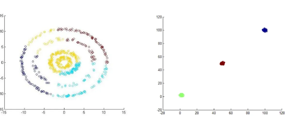
popularity of the k-means algorithm very few theoretical guarantees on its performance are known. In practice however, k-means performs well on data that at least approximately follows its assumption of being generated by a mixture of well-separated spherical Gaussians [20]. This, coupled with its simplicity makes it a handy tool for a data-miner. However, k-means performs poorly when these assumptions of data generation are not met, which is usually the case in real world datasets. Figure 1.1 shows the results of using k-means on two synthetic datasets. k-means is unable to identify clusters when the data is distributed in concentric groups (left figure in Figure 1.1), while it clearly finds the clusters in well separated and tight spherical Gaussians (right). The clusters identified are indicated by different colors. Both sets have 600 points. Spectral Clustering makes no such assumptions for data generation. It instead finds groupings by analyzing the top eigenvectors of the affinity matrix and hence usually returns better results.
Note that the broad idea of clustering is essentially to group points that are similar in one cluster and points that are dissimilar into different clusters. The notion of similarity that is employed in k-means is the Euclidean distance between data points and the cluster centroids to which they are assigned to (which get updated in each iteration). In a sense, the idea of similarity used in k-means restricts what could be known about the geometry of the data. In k-means we work with the data directly, in spectral clustering however, we work with a representation of the data that gives a more global (and hence better) encoding
CHAPTER 1. PRELIMINARIES 9
Figure 1.1: Results of using k-means on two synthetic datasets.
of the similarities between points. This similarity in spectral clustering is represented in the form of a graph called the similarity graph, represented byG = (V, E) whereV is the set of vertices andE is the set of edges. The idea is that points in the dataset can be represented by a graph with each data point as a vertex of the graphG and the edges connecting them encoding a notion of similarity wij > 0 between them. Two points are connected in the
graph if the similarity or weight between them is either non-zero or above some threshold. The clustering problem can then be re-stated using information from the similarity graph as: We want to find partitions of this graph such that weights between points in the same group are high and those between points in different groups are low. Before talking how we cluster using this representation, we introduce some notation and discuss how the graph is used to represent the dataset.
Given the similarity graph G of n data points {x1, x2. . . xn}, there are essentially two
things about it that tell us something about the global structure of the data:
1. The degree of a vertex (a data-point in our case): The degree of a vertex tells us the sum of weights of all the edges that originate from a vertex i to all other vertices j. It is given by: di= n X j=1 wij
This definition is somewhat non-standard but more general. The standard definition for degree of a vertex is only defined for wij ={0,1}, and thus is only the count of
CHAPTER 1. PRELIMINARIES 10
the similarity graph is the diagonal matrix Dwith the degrees di on the diagonal.
D= d1 d2 . .. dn
Intuitively the degree matrix of a graph tells us how many points each point is con-nected to (we could connect all points, or choose to connect k-nearest neighbors of each point) and by how much (hence the summation of the weights).
2. The weighted similarity matrix or the affinity matrix of the similarity graph, W on the other hand is a representation of similarity between all the points. Each element in the affinity matrix is given bywi.j, which is the weight or edge between two points iand j. A common way of representing the weight is:
wij =exp − xi−xj 2 2σ2 !
Notice that wi,j is simply the exponentiated Euclidean distance between two points
(points in Rn ) scaled by a parameter called the scaling or weighing parameter σ .
This parameter is to be tuned and varying it changes the weight between points. A point to note is that if all the points are connected then allwi,j such that i6=j will
be non-zero values. If points are connected to only their k-nearest neighbors and not every other point, then most of the matrix W will be populated with zeroes.
The matricesW andDtell us something about the global structure of the data, but we dont work with them directly. We instead work with the graph Laplacian matrix given by
L=D−W
The above is the un-normalized version of the Laplacian. There are two normalized versions that are represented as:
Lsym=D−1/2W D−1/2
and
CHAPTER 1. PRELIMINARIES 11
The first is called the symmetric Laplacian while the second is called the random-walk Laplacian. The Laplacian in a way combines both the degree and the affinity matrix and also has some mathematically interesting properties (such as being positive semi-definite) that make it easier to work with [75]. Since the Laplacian is a representation of the similarity between the data-points, we can now work with it to find groups in the data. Given the above background, clusters in a dataset can be found by the following method[78]:
A Spectral Clustering Algorithm due to Ng, Jordan, Weiss [78]:
1. For the dataset having ndata points, construct the similarity graph G. The similarity graph can be constructed in two ways: by connecting each data point to the other
n−1 data points or by connecting each data point to its k-nearest neighbors. A rough estimate of a good value of the number of nearest neighbors is log(n). The similarity between the points is given bywij =exp −
xi−xj 2 2σ2 !
. This will give the matrixW.
2. Given the similarity graph, construct the degree matrix D.
3. Using D and W findLsym.
4. Let K be the number of clusters to be found. Compute the first K eigenvectors of
Lsym. Sort the eigenvectors according to their eigenvalues.
5. If u1, u2...uK are the top eigenvectors of Lsym, then construct a matrix U such that U ={u1, u2. . . uK}. Normalize rows of matrix U to be of unit length.
6. Treat the rows in the normalized matrix U as points in a K dimensional space and use k-means to cluster these.
7. If c1, c2. . . cK are the K clusters, Then assign a point in the original dataset si to
cluster cK if and only if the ith row of the normalized U is assigned to clustercK.
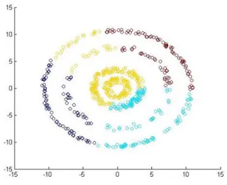
It is noteworthy that we dont cluster the original dataset directly. We first transform it to find its top K eigenvectors. These being the most important eigenvectors of L, encode the maximum information about it. At the same time, this reduces the dimensionality which without throwing away much information which makes the task of clustering much
CHAPTER 1. PRELIMINARIES 12
Figure 1.2: Results of using Spectral Clustering on a synthetic dataset.
easier. To illustrate the power given by this change of representation, we demonstrate it on a toy dataset (Figure 1.2). A detailed tutorial that explains various spectral clustering algorithms and some point of views on why it works is by Luxburg[71].
1.2.1 Self-Tuning Spectral Clustering
One major issue with the Spectral Clustering algorithms suggested before 2005 was that they were usually not suitable for handling multi-scale data. The associated parameter that handled scaling had to be learned by cross-validation. This parameter is the parameter σ
in the equation below:
wij =exp − xi−xj 2 2σ2 !
Many times, for cluster analysis true cluster labels are not known which restricted the utility of spectral clustering algorithms. An important development was the suggestion
of using Local Scaling for the selection of an appropriate σ by Zelnik-Manor and Perona
[102]. Choosingσ by cross-validation had many issues - Data which had clusters at various scales would usually have a different σ associated and hence using the same for the entire dataset would result in bad results overall. At the same time, since σ had to be learned by cross-validation, other than the increased time and computational resources needed for the same, the initial guess for searching it had to be done manually. [102] suggested using local scaling in the following way to over come this problem: Instead of selecting a single
CHAPTER 1. PRELIMINARIES 13
scaling parameter for the entire dataset they proposed calculating a scaling parameter σi
for each data point xi What this would imply that for the a distance between two points
could be represented asymmetrically. The distance to pointxj from pointxi would be given
as d(xi,xj)
σi and the distance to point xi from xj would be given by
d(xj,xi)
σj . The squared
distance could then be appropriately written as:
d2(xi, xj) σiσj
. Thus the affinity between two points could be written as
wij =exp −d2(x i,xj) σiσj
The good thing about this formulation is that each σ could be calculated based on the
local statistics of each point, completely eliminating the need of finding the same by cross validation. Thus, the algorithm due to Ng., Jordan, and Weiss could be modified with this change in calculating the affinity matrix. Experimental results using Self-Tuning generally returns better results.
14
Part II
15
Chapter 2
Motivation to Regularity
Clustering
2.1
Introduction
The Regularity lemma of Szemer´edi [92] has proved to be a very useful tool in graph theory. It was initially developed as an auxiliary lemma to prove a long standing conjecture of Erd˝os and Tur´an on arithmetic progressions [39] , which stated that sequences of integers with positive upper density must contain arbitrarily long arithmetic progressions. Now the Regularity Lemma by itself has become an important tool and found numerous other applications (see [69]). Based on the Regularity Lemma and the Blow-up Lemma [67], [68] the Regularity method has been developed that has been quite successful in a number of applications in graph theory (e.g. [56], [57]).
However, one major disadvantage of these applications and the Regularity Lemma is that they are mainly theoretical, they work only for astronomically large graphs as the Regularity Lemma can be applied only for such large graphs. Indeed, to find the ε-regular partition in the Regularity Lemma, the number of vertices must be a tower of 2’s with height proportional toε−5. Furthermore, Gowers demonstrated [52] that a tower bound is necessary.
The basic content of the Regularity Lemma could be described by saying that every graph can, in some sense, be partitioned into random graphs. Since random graphs of
CHAPTER 2. MOTIVATION TO REGULARITY CLUSTERING 16
a given edge density are much easier to treat than all graphs of the same edge-density, the Regularity Lemma helps us to carry over results that are trivial for random graphs to the class of all graphs with a given number of edges. We are especially interested in harnessing the power of the Regularity Lemma for clustering data. Graph partitioning methods for clustering and segmentation have become quite popular in the past decade because of the ease of representations and interactions with graphs and the theoretical underpinnings for clustering provided by spectral graph theory. The Regularity Lemma is a result that comes with important theoretical implications and thus importing it into machine learning for clustering could potentially have many advantages. An earlier attempt to apply the Regularity Lemma in real-world applications can be found in [90], but the authors do not provide too many details.
In this part we propose a general methodology to make the Regularity Lemma more useful in practice. To make it truly applicable, instead of constructing a provably regular partition we construct an approximately regular partition. This partition behaves just like a regular partition (especially for graphs appearing in practice) and yet it does not require
the large number of vertices as mandated by the original Regularity Lemma. We will
call this Practical Regularity Lemma. Then this approximately regular partition is used for performing clustering and image segmentation. We call the resulting new clustering technique Regularity clustering. We present comparisons with standard pairwise clustering methods such ask-means and spectral clustering and the results are very encouraging
To present our results, this part is organized as follows. In Section 2.2 we discuss clustering in general and also present a popular spectral clustering algorithm that is used later in the reduced graph. We also point out what are the possible ways to improve its running time. In Section 3.1 we give some definitions and general notation. In Chapter 3 we present the Regularity Lemma, first the original form (which was non-constructive) and two well known constructive versions that were proved much later. Furthermore, in this section we point out the various problems arising when we attempt to apply the lemma in real-world applications and a general outline of how the Regularity Lemma is used in establishing theoretical results. In Section 4.1 we discuss how the constructive Regularity Lemma could be modified to make it truly applicable for real-world problems where the graphs typically
CHAPTER 2. MOTIVATION TO REGULARITY CLUSTERING 17
are much smaller, say have a few thousand vertices only. In Section 4.2 we show how this Practical Regularity Lemma can be applied to develop a new clustering technique called Regularity clustering. In Section 4.3, we present an extensive empirical validation of our method and also present comparisons with methods such as spectral clustering. Section 4.4 is spent in discussing the various possible future directions of work.
2.2
Clustering
It is fair to say that at least some part of our understanding of the world is by a semi-supervised learning process that involves some sort of clustering. Not surprisingly it has been often pointed out that a mathematically precise understanding of clustering could go a long way in helping us solve problems at least approximately as solved by the brain [91]. Clustering is perhaps the most used data mining tool for exploratory data analysis. It’s uses are primarily in finding meaningful groups, for feature extraction and summarizing and using it for making data-driven inferences. An useful view of clustering is the following: Given a spaceX, clustering could be thought of as a partitioning of this space intoK parts
i.e. f :X 7−→ {1, . . . , K}. Usually this partitioning is obtained by optimizing some internal
criteria such as the inter-cluster distances, etc.
Out of the various modern clustering techniques, spectral clustering has become one of the most popular. This has happened due to not only its superior performance over the traditional clustering techniques, but also due to the strong theoretical underpinnings in spectral graph theory and its ease of implementation. It has many advantages over the
more traditional clustering methods such ask-means and expectation maximization (EM).
The most important is its ability to handle datasets that have arbitrary shaped clusters.
Methods such as k-means and EM are based on estimating explicit models of the data.
Such methods fail spectacularly when the data is organized in very irregular and complex clusters. Spectral clustering on the other hand does not work by estimating explicit models of the data. It analyzes the spectrum of the graph Laplacian obtained from the pairwise similarities of the data points (similarity matrix). This is useful as the top few eigenvectors can unfold the data manifold to form meaningful clusters [104].
CHAPTER 2. MOTIVATION TO REGULARITY CLUSTERING 18
In this work we employ spectral clustering on the reduced graph, even though any other pairwise clustering method could be used. The algorithm that we employ is due to Ng, Jordan and Weiss [78]. Despite various advantages of spectral clustering, one major problem is that for large datasets it is very computationally intensive. And understandably this has received a lot of attention recently. In the form of spectral clustering that is originally stated there are two main bottlenecks: First, the finding of the affinity matrix of the pairwise distances between datapoints, and second, once we have the affinity matrix
the finding of the eigendecomposition. Many ways have been suggested to solve these
problems. One approach is not to use an all-connected graph but a k-nearest neighbour graph in which each data point is typically connected to lognneighboring datapoints(where
n is the number of data-points). This considerably speeds up the process of finding the
affinity matrix, however it has a drawback that by taking nearest neighbors we might miss something interesting in the global structure of the data. A method to remedy this is the
Nystr¨om method which takes a random sample of the entire dataset (thus preserving the
global structure in a sense) and then doing spectral clustering on this much smaller sample. The results are then extended to all other points in the data set [46], [8].
Our work is quite different from such methods. The speed-up is primarily in the second stage where eigendecomposition is to be done. The original graph is represented by a reduced graph which is much smaller and hence the resulting affinity matrix is much smaller reducing the computational load. Further work on a practical variant of the sparse Regularity Lemma could be useful in a speed-up in the first stage, too.
2.3
Prior Attempts to Use the Regularity Lemma for
Prac-tical Applications
Given the astronomical bounds associated with the Regularity Lemma and moreover since Gowers established that they are necessary [52], the practical applications of the Regularity Lemma have been non-existent. Indeed, many times some indirect applications are alluded to. A recent exposition on the work of Endre Szemer´edi by Gowers [53] gives an instance of an indirect practical application that could be particularly useful. This is in relation to
CHAPTER 2. MOTIVATION TO REGULARITY CLUSTERING 19
the Probably-Approximately-Correct or simply PAC formalism advanced by Leslie Valiant [99], a very useful way of thinking about machine learning. However, no results concerning the Regularity Lemma and it’s application to the PAC Learning formalism are known.
Another recent line of investigation that might eventually be relevant to Machine Learn-ing is due to Csisz´ar-Rejt¨o-Tusn´ady [27]. In this work they investigate the utility of the Regularity Lemma with respect to statistical inference on random structures and also give an interpretation of the Regularity Lemma for the statistician.
In more practical applications a recent work by Nepusz et al. [76] involves prediction of yet uncharted connections in the large scale network of the cerebral cortex. They give an interesting way to solve this problem by a method that claims inspiration from the
Regularity Lemma. In another paper by Nepusz and Basz´o, the Regularity Lemma is again
used as an inspiration as in [76] for developing an algorithm for clustering of Directed Graphs [77]. Pehkonen and Reittu [82] also use the Regular Partition promised by the Regularity Lemma as an inspiration to develop a strategy to cluster peer-to-peer streaming data. However, note that none of the above applications use the Regularity Lemma directly, they only use the Regularity Lemma as an inspiration to come up with a similar working methodology.
The only practical application of the Regularity Lemma to the best of our understanding remains by Sperotto & Pelillo [90], where they use the Regularity Lemma as a pre-processing step. They give some interesting ideas on how the Regularity Lemma might be used, however they don’t give too many details on the same. In subsequent chapters we give an attempt to harness the power of the Regularity Lemma for the practical task of clustering. We begin with some background on the Regularity Lemma in the next chapter.
20
Chapter 3
The Szemer´
edi Regularity Lemma
The Regularity Lemma is a cornerstone result in Extremal Graph theory with wide ranging implications and applications. It’s fundamental nature can be understood by considering that it has an important place in linking many area of mathematics, such as analysis and combinatorics. The Regularity Lemma was originally advanced as a tool in the original proof in 1975 by Endre Szemer´edi of an old conjecture of Erd˝os and Tur´an on Ramsey Properties of arithmetic progressions [39].
The purpose of this chapter is to introduce the Regularity Lemma. It must be noted that the statement of the Lemma as originally stated is an existential, non-constructive one. If we have to work towards making the Regularity Lemma truly applicable to settings in clustering, then we first need an algorithmic version and then make changes to that. Here we review the original statement of the Regularity Lemma and it’s constructive versions. However, before doing so, we introduce some definitions and notations.
3.1
Definitions and Notation
Let G = (V, E) denote a graph, where V is the set of vertices and E is the set of edges. When A, B are disjoint subsets ofV, the number of edges with one endpoint in Aand the other in B is denoted by e(A, B). When A and B are nonempty, we define the density of
edges between A andB as
d(A, B) = e(A, B) |A||B| .
CHAPTER 3. THE SZEMER ´EDI REGULARITY LEMMA 21
The most important concept is the following.
Definition 1. The bipartite graph G= (A, B, E) is ε-regular if for every X ⊂A, Y ⊂ B
satisfying
|X|> ε|A|, |Y|> ε|B|
we have
|d(X, Y)−d(A, B)|< ε,
otherwise it isε-irregular.
Roughly speaking this means that in an ε-regular bipartite graph the edge density
betweenanytwo relatively large subsets is about the same as the original edge density. In effect this implies that all the edges are distributed almost uniformly.
Definition 2. A partitionP of the vertex setV =V0∪V1∪. . .∪Vk of a graph G= (V, E)
is called an equitable partition if all the classes Vi,1≤i≤k, have the same cardinality. V0
is called the exceptional class.
Thus note that the exceptional class V0 is there only for a technical reason, namely to guarantee that the other classes have the same cardinality.
Definition 3. For an equitable partition P of the vertex set V = V0 ∪V1 ∪. . .∪Vk of G= (V, E), we associate a measure called the index of P (or the potential) which is defined by ind(P) = 1 k2 k X s=1 k X t=s+1 d(Cs, Ct)2.
This will measure the progress towards an ε-regular partition.
Definition 4.An equitable partitionP of the vertex setV =V0∪V1∪. . .∪Vk ofG= (V, E)
is called ε-regular if |V0| < ε|V| and all but εk2 of the pairs (Vi, Vj) are ε-regular where
1≤i < j ≤k.
CHAPTER 3. THE SZEMER ´EDI REGULARITY LEMMA 22
3.2
Original Statement
The Regularity Lemma essentially states that every large enough graph could be approxi-mated by the union of a constant number of bipartite graph. A detailed exposition to some statements and applications of the Regularity Lemma can be found here [69].
More specifically this lemma claims that every (dense) graph could be partitioned into
a bounded number of pseudo-random bipartite graphs and a few leftover edges. Since
random graphs of a given edge density are much easier to treat than all graphs of the same edge-density, the Regularity Lemma helps us to translate results that are trivial for random graphs to the class of all graphs with a given number of edges.
Theorem 1 (Szemer´edi Regularity Lemma [92]). For every positive ε >0 and posi-tive integer t there is an integerT =T(ε, t) such that every graph with n > T vertices has anε-regular partition into k+ 1classes, where t≤k≤T.
3.3
Algorithmic Versions of the Regularity Lemma
The original proof of the regularity lemma [92] does not give a method to construct a regular partition but only shows that one must exist. To apply the regularity lemma in practical settings, we need a constructive version. Alonet al. [2] were the first to give an algorithmic version. Since then a few other algorithmic versions have also been proposed [48], [64]. Below we present the details of the Alon et al. algorithm.
3.3.1 Alon-Duke-Lefmann-R¨odl-Yuster Version
Theorem 2 (Alon et al. Algorithmic Regularity Lemma [2]). For every ε > 0 and every positive integer t there is an integer T = T(ε, t) such that every graph with n > T
vertices has an ε-regular partition intok+ 1classes, wheret≤k≤T. For every fixedε >0
and t ≥ 1 such a partition can be found in O(M(n)) sequential time, where M(n) is the time for multiplying two nby nmatrices with 0,1 entries over the integers. The algorithm can be parallelized and implemented in N C1.
CHAPTER 3. THE SZEMER ´EDI REGULARITY LEMMA 23
This result is somewhat surprising from a computational complexity point of view since as it was proved in [2] the corresponding decision problem (checking whether a given parti-tion isε-regular) isco−N P-complete. Thus the search problem is easier than the decision problem.
Theorem 3 [2]. The Following decision problem is co−N P-complete: Given a Graph G, an integerk≥1 and a parameterε >0, and a partition of the set of vertices ofG in k+ 1
parts. Decide is the given partition is ε-regular.
To describe the algorithm underlined in Theorem 2 and how it is an algorithm in the first place, we first introduce a couple of definitions:
Definition 5 (Average Degree).
If H is a bipartite graph with classes of equal size |A| = |B| = n. Then, the average degree of H may be given as:
d= 1 2n
X
i∈A∪B deg(i)
Definition 6 (Neighborhood Deviation) [2].Lety1 andy2 be two distinct vertices, such
thaty1, y2 ∈B. The neighborhood deviation of y1, y2 is defined as:
σ(y1, y2) =|N(y1)∩N(y2)| −
d n2
Where N(.) gives the neighborhood of a vertex. For some subset Y ⊆B, the deviation of this set Y is defined as:
σ(Y) = P
y1,y2∈Y σ(y1, y2)
|Y|2
Now given that 0< ε < 161 and if Y ⊆B and is sufficiently large i.e|Y|> εn and such thatσ(Y)≥ ε3n
2 , then one the following conditions holds: 1. d < ε3ni.e. H isε-irregular
2. There exists inB a set of atleast 18ε4n. The degrees of this set deviate fromdby at leastε4n
3. There are subsets A0 ⊆A, B0 ⊆B,|A0| ≥ ε4
4n,|B
0| ≥ ε4
4n and |d(A
0, B0)−d(A, B)| ≥
CHAPTER 3. THE SZEMER ´EDI REGULARITY LEMMA 24
It is using these cases that the algorithm mentioned in Theorem 2 can be derived. To describe the actual algorithm we need a couple of more Lemmas.
Lemma 1 (Alon et al. [2]). Let H be a bipartite graph with equally sized classes |A|= |B| = n. Let 2n−1/4 < ε < 161. There is an O(M(n)) algorithm that verifies that H
is ε-regular or finds two subset A0 ⊂ A, B0 ⊂ B, |A0| ≥ ε164n, |B0| ≥ ε164n, such that
|d(A, B)−d(A0, B0)| ≥ε4. The algorithm can be parallelized and implemented in N C1.
This lemma basically says that we can either verify that the pair is ε-regular or we provide certificates that it is not. The certificates are the subsets A0, B0 and they help to proceed to the next step in the algorithm. The next lemma describes the procedure to do the refinement from these certificates.
Lemma 2 (Szemer´edi [92]). Let G = (V, E) be a graph with n vertices. Let P be an equitable partition of the vertex set V = V0 ∪V1 ∪. . .∪Vk. Let γ > 0 and let k be a
positive integer such that 4k > 600γ−5. If more than γk2 pairs (Vs, Vt), 1 ≤ s < t ≤ k,
are γ-irregular then there is an equitable partition Q of V into 1 +k4k classes, with the cardinality of the exceptional class being at most
|V0|+
n
4k
and such that
ind(Q)> ind(P) +γ 5 20.
This lemma implies that whenever we have a partition that is not γ-regular, we can
refine it into a new partition which has a better index (or potential) than the previous partition. The refinement procedure to do this is described below.
Refinement Algorithm: Given a γ-irregular equitable partition P of the vertex set
V =V0∪V1∪. . .∪Vk with γ= ε
4
16, construct a new partition Q.
For each pair (Vs, Vt), 1 ≤s < t ≤k, we apply Lemma 1 with A =Vs, B = Vt and ε. If
(Vs, Vt) is found to be ε-regular we do nothing. Otherwise, the certificates partition Vs and Vt into two parts (namely the certificate and the complement). For a fixed swe do this for
CHAPTER 3. THE SZEMER ´EDI REGULARITY LEMMA 25
namely two elements are equivalent if they lie in the same partition set for every t 6= s. The equivalence classes will be called atoms. Set m =b|Vi|
4kc, 1≤i≤k. Then we choose a
collection Q of pairwise disjoint subsets of V such that every member of Q has cardinality
m and every atomA contains exactlyb|mA|c members ofQ. The collectionQ is an equitable partition ofV into at most 1 +k4k classes and the cardinality of its exceptional class is at most |V0|+4nk.
Now we are ready to present the main algorithm.
Regular Partition Algorithm: Given a graph G and ε, construct a ε-regular parti-tion.
1. Initial partition: Arbitrarily divide the vertices of G into an equitable partition P1
with classes V0, V1, . . . , Vb, where |V1|=bnbc and hence |V0|< b. Denote k1=b.
2. Check regularity: For every pair (Vs, Vt) of Pi, verify if it is ε-regular or find X⊂Vs, Y ⊂Vt,|X| ≥ ε
4
16|Vs|,|Y| ≥
ε4
16|Vt|, such that |d(X, Y)−d(Vs, Vt)| ≥ε4.
3. Count regular pairs: If there are at mostεki2 pairs that are not verified asε-regular, then halt. Pi is an ε-regular partition.
4. Refinement: Otherwise apply the Refinement Algorithm and Lemma 2, where P =
Pi, k=ki, γ= ε
4
16, and obtain a partition Q with1 +ki4ki classes.
5. Iteration: Let ki+1 =ki4ki, Pi+1 =Q, i=i+ 1, and go to step 2.
Since the index cannot exceed 1/2, the algorithm must halt after at most d10γ−5e iterations (see [2]). Unfortunately, in each iteration the number of classes increases to
k4k from k. This implies that the graph G must be indeed astronomically large (a tower function) to ensure the completion of this procedure. As mentioned before, Gowers [52]
proved that indeed this tower function is necessary in order to guarantee an ε-regular
partition for allgraphs. The size requirement of the algorithm above makes it impractical for real world situations where the number of vertices typically is a few thousand.
In the next section we describe the constructive version of the Regularity Lemma due to Frieze and Kannan [48].
CHAPTER 3. THE SZEMER ´EDI REGULARITY LEMMA 26
3.3.2 Frieze-Kannan Version
To describe this algorithm we need Lemma 2, the definitions in Section 3.1 and another lemma that we state below.
Lemma 3 (Frieze-Kannan [48]) Let W be an R×C matrix with |R|= p and |C| =q
and W
∞ and let γ be a positive real.
a If there exists S ⊆ R, T ⊆ C such that |S| ≥ γp,|T| ≥ γq and |W(S, T)| ≥ γ|S||T|
thenσ1(W)≥γ3√pq. Where σ1 is the first singular value.
b If σ1(W) ≥ γ√pq then there exist S ⊆R, T ⊆C such that |S| ≥ γ0p,|T| ≥ γ0q and
W(S, T)≥γ0|S||T|, where γ0 = 108γ3 . Also S, T can be constructed in Polynomial time by the method of conditional expectation [83], [89]
Combining the Lemmas 2 and 3, we get an algorithm for finding an epsilon regular partition, quite similar to the Alon et al. version [2], which we present below:
Regular Partition Algorithm (Frieze-Kannan): Given a graphGandε, construct a ε-regular partition.
1. Initial partition: Arbitrarily divide the vertices of G into an equitable partition P1
with classes V0, V1, . . . , Vb, where |V1|=bnbc and hence |V0|< b. Denote k1=b.
2. Check regularity: For every pair (Vs, Vt) of Pi, compute σ1(Wr,s). If the pair
(Vr, Vs) are not ε-regular then by Lemma 3 we obtain a proof that they are not not γ =ε9/108-regular.
3. Count regular pairs: If there are at most εk2
i pairs that produce proofs of non γ-regularity, then halt. Pi is an ε-regular partition.
4. Refinement: Otherwise apply the Refinement Algorithm and Lemma 2, where P =
Pi, k=ki, γ= ε
9
108, and obtain a partition P
0 with1 +k
i4ki classes.
5. Iteration: Let ki+1 =ki4ik, Pi+1 =P0, i=i+ 1, and go to step 2.
This algorithm is guaranteed to finish in at most ε−45 steps with anε-regular partition. In the next section we outline some basic ideas that are used to apply the Regularity Lemma.
CHAPTER 3. THE SZEMER ´EDI REGULARITY LEMMA 27
3.4
Using the Regularity Lemma
In applications of the Regularity Lemma the concept of thereduced graphplays an important role.
Definition 7 Given an ε-regular partition of a graph G= (V, E) as provided by Theorem 1, we define the reduced graph GR as follows. The vertices of GR are associated to the classes in the partition and the edges are associated to the ε-regular pairs between classes with density above d.
The most important property of the reduced graph is that many properties of G are
inherited byGR. ThusGRcan be treated as a representation of the original graphGalbeit with a much smaller size, an “essence” of G. Then if we run any algorithm onGR instead of Gwe get a significant speed-up.
An instance of using the Regularity Lemma via the concept of a reduced graph is
the so called Regularity Lemma-Blow-Up Lemma Method developed by Koml´os-S´ark¨
ozy-Szemer´edi [67]. The rough outline of the method involves first applying the Regularity Lemma to the graph and obtaining the reduced graph. Given that it has properties as outlined above, knowing the density conditions in the reduced graph we can find nice objects (these depend on the particular application and density condition, triangles, cliques, etc.) in it by applying usually well-known or easy extremal graph theoretical results. The goal is to reduce the embedding problem in the original graph to embedding into these regular objects in the partitioning. For this purpose sometimes we have to do some technical steps, such as connecting these objects (if for example we are looking for a Hamiltonian cycle) or eliminating the various exceptional vertices, etc. For the last step of the method, for the embedding into the regular objects, the Blow-up Lemma [67] is used.
However, the use of the reduced graph is mainly in establishing theoretical results. In the next chapter we suggest some changes to the Regular Partition algorithm described in the previous section so that it could be made more applicable to smaller graphs.
28
Chapter 4
Regularity Clustering
4.1
Modifications to the Constructive Version
To make the regularity lemma applicable we first needed a constructive version that we stated above. But we see that even the constructive version is not directly applicable to real world scenarios. We note that the above algorithm has such restrictions because it’s aim is to be applicable to allgraphs. Thus, to make the regularity lemma truly applicable we
would have to give up our goal that the lemma should work for everygraph and should be
content with the fact that it works formostgraphs. To ensure that this happens, we modify the Regular Partition Algorithm so that instead of constructing a regular partition, we find an approximately regular partition. Such a partition should be much easier to construct. We have the following 3 major modifications to the Regular Partition Algorithm.
Modification 1: We want to decrease the cardinality of atoms in each iteration. In the above Refinement Algorithm the cardinality of the atoms may be 2k−1, where k is the number of classes in the current partition. This is because the algorithm tries to find all the possible ε-irregular pairs such that this information can then be embedded into the subsequent refinement procedure. Hence potentially each class may be involved with up to
k−1 ε-irregular pairs. One way to avoid this problem is to bound this number. To do
so, instead of using all theε-irregular pairs, we only use some of them. Specifically, in this paper, for each class we consider at most oneε-irregular pair that involves the given class. By doing this we reduce the number of atoms to at most 2. We observe that in spite of the
CHAPTER 4. REGULARITY CLUSTERING 29
crude approximation, this seems to work well in practice.
Modification 2: We want to bound the rate by which the class size decreases in each iteration. As we have at most 2 atoms for each class, we could significantly increasemused in the Refinement Algorithm asm = |Vi|
l , where a typical value of l could be 3 or 4, much
smaller than 4k. We call this user defined parameterlthe refinement number.
Modification 3: Modification 2 might cause the size of the exceptional class to increase too fast. Indeed, by using a smaller l, we risk putting 1l portion of all vertices into V0 after
each iteration. To overcome this drawback, we “recycle” most of V0, i.e. we move back
most of the vertices from V0. Here is the modified Refinement Algorithm.
Modified Refinement Algorithm: Given a γ-irregular equitable partition P of the vertex set V = V0 ∪V1∪. . .∪Vk with γ = ε
4
16 and refinement number l, construct a new
partition Q.
For each pair (Vs, Vt), 1≤s < t≤k, we apply Lemma 1 with A=Vs, B =Vt and ε. For
a fixed sif (Vs, Vt) is found to be ε-regular for allt6=swe do nothing, i.e. Vs is one atom.
Otherwise, we select one ε-irregular pair (Vs, Vt)randomly and the corresponding certificate
partitions Vs into two atoms. Set m = b
|Vi|
l c, 1 ≤ i ≤ k. Then we choose a collection Q0 of pairwise disjoint subsets of V such that every member of Q0 has cardinality m and every atom A contains exactly b|mA|c members of Q0. Then we unite the leftover vertices in each Vs, we select one more subset of size m from these vertices and add these sets to Q0
resulting in the partition Q. The collection Q is an equitable partition of V into at most
1 +lk classes.
Now we present our modified Regular Partition Algorithm. There are three main pa-rameters to be selected by the user: ε, the refinement number l and h the minimum class size when we must halt the refinement procedure. h is used to ensure that if the class size has gone too small then the procedure should not continue.
Modified Regular Partition Algorithm (or the Practical Regularity Lemma):
Given a graph Gand parameters ε, l, h, construct an approximately ε-regular partition. 1. Initial partition: Arbitrarily divide the vertices of G into an equitable partition P1
CHAPTER 4. REGULARITY CLUSTERING 30
with classes V0, V1, . . . , Vl, where |V1|=bnlc and hence |V0|< l. Denote k1 =l.
2. Check size and regularity: If |Vi|< h, 1≤i≤k, then halt. Otherwise for every
pair (Vs, Vt) of Pi, verify if it is ε-regular or find X ⊂Vs, Y ⊂Vt,|X| ≥ ε
4
16|Vs|,|Y| ≥
ε4
16|Vt|, such that |d(X, Y)−d(Vs, Vt)| ≥ε 4.
3. Count regular pairs: If there are at mostεki2 pairs that are not verified asε-regular, then halt. Pi is an ε-regular partition.
4. Refinement: Otherwise apply the Modified Refinement Algorithm, whereP =Pi, k= ki, γ = ε
4
16, and obtain a partition Q with1 +lki classes.
5. Iteration: Let ki+1 =lki, Pi+1=Q, i=i+ 1, and go to step 2.
4.2
A Two Phase Strategy for Clustering
To make the regularity lemma applicable in clustering settings, we adopt the following two phase strategy (Figure 4.1):
1. Application of the Practical Regularity Lemma: In the first stage we apply the practical regularity lemma as described in the previous section to obtain an approxi-mately regular partition of the graph representing the data. Once such a partition has been obtained, the reduced graph as described in Definition 7 could be constructed from the partition.
2. Clustering the Reduced Graph: The reduced graph as constructed above would preserve most of the properties of the original graph (see [69]). This implies that any changes made in the reduced graph would also reflect in the original graph. Thus, clustering the reduced graph would also yield a clustering of the original graph. We apply spectral clustering (though any other pairwise clustering technique could be used) on the reduced graph to get a partitioning and then project it back to the higher dimension. Recall that vertices in the exceptional setV0, are leftovers from the refinement process and must be assigned to the clusters obtained. Thus in the end these leftover vertices are redistributed amongst the clusters using k-nearest neighbour classifier to get the final grouping.
CHAPTER 4. REGULARITY CLUSTERING 31
Figure 4.1: A Two Phase Strategy for Clustering
4.3
Empirical Validation
In this section we present extensive experimental results to indicate the efficacy of this approach both by employing it for clustering on a number of benchmark datasets and for the task of image segmentation. We also compare the results with spectral clustering (both for the fully connected graph and k-nearest neighbour graphs) in terms for accuracy. We also report some results that indicate the amount of compression obtained by constructing the reduced graph.
As discussed later, the results also directly point to a number of promising directions of future work. We first review the datasets considered and the metrics used for comparisons.
4.3.1 Datasets and Metrics Used
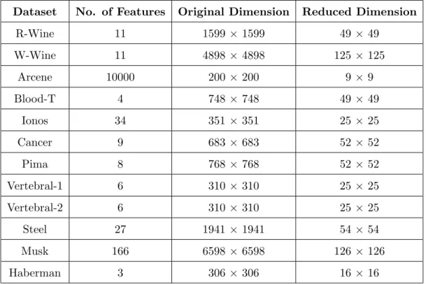
The datasets considered for empirical validation were taken from the University of Califor-nia, Irvine machine learning repository [47]. A total of 12 datasets were used for validation. We considered datasets with real valued features and associated labels or ground truth. In some datasets (as described below) that had a large number of real valued features, we removed categorical features to make it easier to cluster. Unless otherwise mentioned, the number of clusters was chosen so as to equal the number of classes in the dataset (i.e. if the number of classes in the ground truth is 4, then the clustering results are for k = 4 etc). An attempt was made to pick a wide variety of datasets i.e. with integer features, binary features, synthetic datasets and of course real world datasets with both very high and small
CHAPTER 4. REGULARITY CLUSTERING 32
dimensionality.
The following datasets were considered: (1) Red Wine (R-Wine) and (2) White Wine (W-Wine) are two datasets having 1599 and 4898 datapoints respectively, each having 11 features. The target measures wine quality on a scale of 0-10. Though both are ten class problems, they only contain labels for 6 and 7 classes respectively. (3) The Arcene dataset (Arcene) has data for the task of distinguishing cancer from normal patterns from mass spectroscopic data. Thus it is a 2-class problem and was used in the NIPS 2003 feature selection challenge. The data consists of a train set with 100 points, a validation set with 100 points and a test set with 700 points (the test set does not come with labels). However, since we are not making any prediction as such we can combine the train and validation sets here and use it as one dataset. Thus, this dataset has 200 datapoints with each data
instance described by 10000 features. Given this very high dimensionality, this should
be an interesting dataset to experi