Generalised Adaptive Fuzzy Rule Interpolation
Longzhi Yang,
Member, IEEE,
Fei Chao,
Member, IEEE,
and Qiang Shen
Abstract—As a substantial extension to fuzzy rule interpo-lation that works based on two neighbouring rules flanking an observation, adaptive fuzzy rule interpolation is able to restore system consistency when contradictory results are reached during interpolation. The approach first identifies the exhaustive sets of candidates, with each candidate consisting of a set of interpolation procedures which may jointly be responsible for the system inconsistency. Then, individual candidates are modified such that all contradictions are removed and thus interpolation consistency is restored. It has been developed on the assumption that contradictions may only be resulted from the underlying interpolation mechanism, and that all the identified candidates are not distinguishable in terms of their likelihood to be the real culprit. However, this assumption may not hold for real world situations. This paper therefore further develops the adaptive method by taking into account observations, rules and inter-polation procedures, all as diagnosable and modifiable system components. Also, given the common practice in fuzzy systems that observations and rules are often associated with certainty degrees, the identified candidates are ranked by examining the certainty degrees of its components and their derivatives. From this, the candidate modification is carried out based on such ranking. This work significantly improves the efficacy of the existing adaptive system by exploiting more information during both the diagnosis and modification processes.
Index Terms—Fuzzy inference, adaptive fuzzy rule interpola-tion, ATMS, GDE.
I. INTRODUCTION
Fuzzy inference systems have been successfully applied to many real world applications, but the systems may suffer from either too sparse or too complex rule bases. Fuzzy rule interpolation (FRI) alleviates this by supporting infer-ence with incomplete sparse rule bases, or by simplifying complex fuzzy systems that involve very dense rule bases through approximating certain parts of the model with their neighbouring rules [1], [2]. Many important FRI methods and their analysis or variations have been presented in the literature, including [1]–[22]. What is common to most of these techniques is that multiple values may be derived for a single variable. This implies that inconsistencies have been generated in the interpolated results.
Adaptive fuzzy rule interpolation(AFRI) was proposed in an
effort to address this problem [23], [24]. It was developed upon FRI approaches by which two neighbouring rules that flank an observation are utilised for interpolation. The approach
L. Yang is with the Department of Computer Science and Digital Tech-nologies, Faculty of Engineering and Environment, Northumbria University, NE1 8ST, UK. e-mail: [email protected].
F. Chao is with the Department of Cognitive Science, School of Infor-mation Science and Engineering, Xaimen University, 361005, China. e-mail: [email protected].
Q. Shen is with the Department of Computer Science, Institute of Mathe-matics, Physics and Computer Science, Aberystwyth University, SY23 3DB, UK. e-mail: [email protected].
efficiently detects inconsistencies, directly locates possible sets of fault components (namely, candidates), and effectively modifies the candidates in order to restore consistency, by removing detected inconsistencies. The approach artificially treats a fuzzy rule interpolation system as a component-based mechanism where system components are defined as interpolation procedures. An assumption-based truth mainte-nance system (ATMS) [25]–[27] is employed to record the depending relationships between interpolated results and their dependent system components (i.e., its proceeding interpola-tion procedures). Then, the classical general diagnostic engine (GDE) [28] is utilised to hypothesise a set of candidates that each may have led to all the system contradictions. Finally, the system consistency is restored by modifying an identified single candidate.
The adaptive approach outlined above assumes that all the contradictory interpolated results are caused by the underpin-ning interpolation procedures. This assumption restricts the applications of AFRI to problems with defective fuzzy inter-polation procedures only, but observations and rules in a fuzzy inference system may also be ill-specified (to a certain extent). Thankfully this limitation is not a fundamental restriction of the idea underlying the adaptive approach. Supported by the initial preliminary investigations of [29], this paper further develops the work of [24], to allow the diagnosis and modifica-tion of observamodifica-tions and rules. This significantly enhances the robustness of the original method as one consistent inference result may still be derived when the original fails, often with intuitively more reasonable interpolated results.
Due to the introduction of more complex and uncertain information to the underlying information and knowledge representation scheme, the number of generated candidates may increase dramatically. However, these candidates can be discriminated as: i) two different values derived for a given variable that have led to a contradiction may not be equally reliable (besides, one may be correct and the other wrong); and ii) all the elements which jointly support one of the two contradictory values may not be equally reliable. A candidate prioritisation mechanism is therefore introduced here to reinforce the present work, starting from the initial report of [30], such that only the most important candidates are considered during the modification stage. Firstly, the classical ATMS is extended to record dependencies and also, to log the extent to which such dependencies are deemed reliable. The candidates are then prioritised using a modified GDE by taking the reliability information into consideration. Thanks to the prioritisation of candidates, a consistent solution can be rapidly derived with saved computational cost.
The remainder of this paper is organised as follows. A brief review of the theoretical underpinnings of AFRI is presented in Sec. II. An extension of the candidate generation procedure
is reported in Sec. III, by which a candidate element can be an observation, rule, or fuzzy interpolation procedure. A generalisation of the candidate modification procedure is discussed in Sec. IV, which allows the modification of all types of diagnosable candidate component. To facilitate comparison, the application problem considered in [24] is reinvestigated in Sec. V where the proposed approach is employed. The paper is concluded in Sec. VI with important future directions of improvements pointed out.
II. ADAPTIVEFUZZYRULEINTERPOLATION
AFRI ensures that interpolated results remain consistent to a certain degree throughout the entire interpolation process [24]. In this paper, given two fuzzy sets Ai and Aj with respect
to the same variable x within the domain Dx, the degree
of consistency between them is represented as the degree of matching as follows:
M(Ai, Aj) = sup
x∈Dx
[min(µAi(x), µAj(x))]. (1) Based on this, the degree β of a contradiction regarding two propositions P (x is Ai) andP′(x is Aj) is defined as:
β = 1−M(Ai, Aj). (2) This work adopts a predefined threshold β0 (0≤β0≤1)to examine whether a pair of values associated with a common variable is unacceptably contradictory. A β0-contradiction appears if the corresponding contradictory degree between the two concerned propositions is greater than β0.
As with [24], each pair of neighbouring rules, which may be utilised together for interpolation, is termed as afuzzy
inter-polation component(FIC). The input of such a component is a
vector of observations and/or previous inferred results, which is hereafter referred to an interpolation input for simplicity. The output is the consequence of the interpolated rule which takes such an input as its antecedent. The working process of AFRI is illustrated in Fig. 1. Given a fuzzy inference problem with a sparse rule base, the interpolator performs inference through fuzzy rule interpolation, and the ATMS records the dependencies of contradictions upon the preceding FICs. Then, the GDE diagnoses the cause of the contradictions and generates candidates for modification, and finally the modifier revises the candidates to remove contradictions and restore system consistency.
ATMS GDE Components Modified Contradiction Dependencies Candidates Beliefs Justifications Modifier Interpolator
Fig. 1. Adaptive fuzzy interpolation
A. Rule Interpolation by the Interpolator Suppose that the interpolation input is
O: x1 =A∗1xand... andxm=A∗mx, (3)
and that rules
Ri: IF x1=A1i and... andxm=Ami, THENy=Bi, Rj: IFx1=A1j and... andxm=Amj, THENy=Bj,
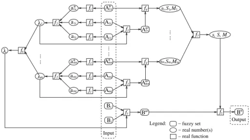
(4) are the neighbouring ones used for interpolation regarding the inputO. The scale and move transformation-based FRI, upon which AFRI has been introduced, is outlined in Fig. 2. Further details of this approach can be found in [12], [13], but this is out of the scope of this paper.
In this figure, there are m repeated sub-components, each of which takesA∗kx,Aki andAkj (1≤k≤m) as inputs and
produces a relative placement factorλk, an intermediate fuzzy set A∗kx′ and a number of similarity measurements between
Akx and A∗kx. Each sub-component first uses the so-called
representative values aki, akj anda∗kx to express the overall
positions of Aki, Akj and A∗kx respectively, computed using the function f1. The relation regarding the relative locations between the interpolation input termA∗kx and the correspond-ing antecedents terms (AkiandAkj) of a pair of neighbouring rules is computed next, resulting in the requiredλk which is computed by the real function f2. From this, an antecedent
term of the intermediate rule A∗kx′ is calculated by applying real functionf3 with a parameterλk toAkiandAkj. Next, a
set of similarity degrees betweenA∗kx andA∗kx′, expressed as the scale ratesk, scale ratioSk and move rateMk, is obtained
by applying the function f4 (which stands for a predefined
similarity metric). Functionf6 is then introduced to combine all the resultant λk (k ∈ {1,2, ..., m}) to an overall single scaleλ, as isf7to combine all the similarity rates (sk,Sk,Mk) to (s,S,M). The conclusion B∗ can finally be approximated by transforming the consequentB∗′ of the intermediate rule. This is implemented by applying the combined single scale similarity rates, through the transformation functionf5:
T(B∗, B∗′) =T((A1x, ...., Amx),(A∗1x′, ...., A∗mx′)). (5)
B. Truth Maintenance by the ATMS
In implementing AFRI, ATMS is utilised to record the dependency of interpolated results and that of contradictions, upon the FICs from which they are inferred. Using ATMS’ terminology, observations, interpolated results, contradictions and FICs can all be represented as ATMS nodes, each of which is formed by a name (standing for its logical or physical meaning), a set of justifications and a label.
Ajustificationexpresses a logical implication through which
a node may be derived from other relevant nodes. An inferred proposition represented as an ATMS node is of the following justification:
M1, M2, ..., Mn, RiRj⇒C, (6) whereRiRjdenotes the FIC formed by the two neighbouring rules Ri andRj (i̸=j) which infers the interpolated result
C from nother nodesM1, M2, ..., Mn (that are observations and/or interpolated results). Based on the definition of con-tradiction, a β0-contradiction is reached if the contradiction degreeβ between any two propositionsP (x is Ai) andP′(x
f2 f1 f1 f1 f2 f1 f1 f1 f4 f4 1 1 1 s ,S ,M mMm S , s m , f5 − fuzzy set real number(s) real function − − Legend: λ λ1 m ... ... 3 ... ... f3 f3 Input A A1i A 1j 1x Ami f a1x 1i a 1j a mx a ami amj f7 Output ... ... Amj mx A s, S, M B B ’* * A ’* * * 1x A ’*mx * * Bi j B f6 λ
Fig. 2. An outline of transformation-based FRI
is Aj) is greater than a predefined threshold β0, which is expressed in the format of proposition as:
P, P′⇒β0⊥. (7)
Alabelis a set of environments, each of which is a minimal
set of FICs that jointly entail the supported node. An environ-ment is said to be β0-inconsistent if β0-contradiction is log-ically derivable by the environment and a given justification; otherwise, the environment is (1−β0)-consistent. The ATMS
label updating algorithm ensures that the label of each node is (1−β0)-consistent, sound, minimal and complete, except
that the label of the special ‘false’ node is β0-inconsistent
rather than (1−β0)-consistent. Whenever a β0-contradiction
is detected, each environment in its label is added into the label of the ‘false’ node and all such environments and their supersets are removed from the label of every other node. Also, any such environment which is a superset of another is removed from the label of the ‘false’ node. Therefore, the label of the special “false” node collectively holds the minimal, complete set of environments each of which leads to a β0 -contradiction.
C. Candidate Generation by the GDE
A set of minimal candidates for modification can be gen-erated by GDE [28] from the label of the ‘false’ node. A candidate is a set of FICs that may have led to all detected contradictions. Since aβ0-inconsistent environment contained in the label of the ‘false’ node indicates that at least one of its elements is inconsistent (or faulty), a candidate must have a non-empty intersection with eachβ0-inconsistent environment. Based on this observation, each candidate is constructed by taking just one FIC from each environment that supports the ‘false’ node. The candidates are guaranteed to be minimal by removing all the supersets of others. As a result of this, the successful correction of any single candidate will remove all contradictions.
D. Candidate Modification by the Modifier
AFRI always modifies the candidate with the smallest cardinality first. With respect to a given queue of candidates
Q, the overall modification procedure is outlined in Alg. 1. The main sub-procedure MODIFY(C) takes a single candidate (C) as input and returns a Boolean value to indicate whether the modification succeeds or not.
Algorithm 1 The CONSISTENCYRESTORINGprocedure CONSISTENCYRESTORING(Q)
Input:Q, a queue of candidates, each of which is a set of FICs.
Output: True, if succeeds;False, otherwise. 1) modif ied←False
2) do
3) C←Dequeue(Q) 4) modif ied← MODIFY(C)
5) while ((modif ied==False) && (Q! =∅)) 6) returnmodif ied
To illustrate the basic ideas embedded in this sub-procedure, suppose that the defective FIC is formed by the pair of neighbouring rules as given in Eq. 4, which flanks the interpo-lation inputs Ox(x∈ {1,2, ..., n})in the form of Eq. 3. The implementation of the modification procedure for a candidate consisting of a single FRI can then be summarised in the following steps:
Step 1. Find the interpolated rule ‘IFx1 =A∗1k and· · · andxm=A∗mk, THENy=Bk∗’ whose antecedent is located in the middle most of the neighbourhood of the antecedents of the two rules used for interpolation, in terms of their representative values that are calculated using a particular integration formula [24]. Suppose that the relative placement
factorof its consequenceλk is modified toλkb . Thecorrection
rate pair can then be calculated as:
{ c−= bλk λk c+=1−bλk 1−λk. (8)
Step 2. Obtain the modified relative placement factors of the consequences of all other interpolated rules, which have been created with respect to the same defective FIC in the same way as that used to compute the correction rate pair above, wherep∈ {1,2, ..., k−1}andq∈ {k+1, k+2, ..., n}:
{ b
λp=λp·c−
1−bλq = (1−λq)·c+.
(9) Step 3. Compute the modified consequences of the in-termediate rules corresponding to all interpolated rules that have been generated from the same defective FIC in accor-dance with their modifiedrelative placement factors. Suppose that the intermediate rule corresponding to defective rule ‘IF x1 = A∗1x and · · · andxm = A∗mx, THEN y = Bx∗’ is ‘IF x1 =A′1xand · · · andxm=A′mx, THENy =Bx′’. From this, the modified consequence of the intermediate rule
b Bx′ is:
b
B′x= (1−bλx)Bi+bλxBj, (10)
wherex∈ {1,2, ..., n}. That is, the modified intermediate rule becomes ‘IFx1=A′1xand · · · andxm=A′mx,THENy=
b Bx′’.
Step 4. Compute the modified consequences of all interpo-lated rules from the consequences of the modified intermediate rules through scale and move transformations:
T((A1x′, ..., Amx′),(A∗1x, ..., A∗mx)) =T(Bbx′,Bbx∗), (11) wherex∈ {1,2, ..., n}, and T(·,·)represents the transforma-tions based on the scale and move measures [12], [13].
Step 5. Impose restriction over the modified consequence such that it becomes consistent with the interpolation context. Suppose thatmobject valuesB1, B2, ..., Bmare obtained for the variabley. If they are(1−β0)-consistent, they must satisfy:
m ∩ j=1
(Bj)β0 ̸=∅, (12) where(Bj)β0 denotes theβ0-cutof fuzzy setBj.
Step 6. Constrain the propagations of all modified conse-quences so that they are consistent with the rest. Propagate the modified result through the entire reasoning network. For a given variable z, suppose that m object values of the variablezhave been modified via the propagation, resulting in modified valuesCib,i∈ {1,2, ..., m}, and thatnobject values
Cj, j ∈ {1,2, ..., n}, ofzare not affected by the propagation. These modified consequences must satisfy the following such that they are all(1−β0)-consistent:
(m ∩ i=1 (Cib)β0 ) ∩(∩n l=1 (Cj)β0 ) ̸ =∅. (13)
Step 7.Solve the set of simultaneous equalities and inequali-ties as posed above. The solutions imply successfully modified results which guarantee the system reasoning consistency.
III. GENERALISINGCANDIDATEGENERATION
Only FICs are regarded as diagnosable and modifiable candidate elements in the original AFRI approach outlined
above. However, observations and rules may also be faulty to a certain extent. This section extends the existing AFRI such that observations and rules can also be diagnosed and modified. To facilitate this, the certainty degrees of observations, rules and FICs are discussed first.
A. Certainty Degrees of Observations and Rules
There are generally four categories of inexact informa-tion [31]: 1) vagueness, 2) uncertainty, 3) both vagueness and uncertainty with the latter represented as real numbers, and 4) both vagueness and uncertainty with the latter also defined as fuzzy sets. The existing FRI [24] only considers type 1 information, which is extended in this work by introducing type 2 information into the system, thereby resulting in the exploitation of type 3 information overall.
With the extra information, an observation is represented as:
O:xi=A∗ij (cO), (14)
where 0 ≤ cO ≤ 1 expresses the certainty degree of the observation O. Conceptually, the vagueness of an object value can be modelled as a fuzzy set due to the lack of a precise boundary between given bits of information. Here, the certainty degree of an observation is represented as a crisp number, which is either assigned subjectively [32] or estimated from other mechanisms such as statistical data analysis. It indicates the confident level at which the current description of the object value may be regarded as of confidence or being reliable.
Denote the certainty degree of an observation O as cO. Then, the uncertainty degree of the same piece of information is naturally expressed as1−cO. Thus, the modifiable range of the object valueO is intuitively bounded to the proportion of 1−cO in reference to the entire variable domain. This means that the factual object value ofO can be obtained by shifting the fuzzy set representation of the defective observation to-wards either side of the variable domain to a maximal distance of 1−cO
2 (maxi−mini), where the domain of the variablexiis Dxi = [mini,maxi]. Given that the shifting of a vague term is restricted from changing the shape and area of the underlying fuzzy set, the shifting process is equivalent to adding a real number to the original fuzzy set [33]. Formally, the factual value of A∗ij, denoted as Ab∗ij, of the observation O as given in Eq. 14 must satisfy:
{ b Aij∗ ≥Aij−1−2cO(maxi−mini) b A∗ij ≤Aij+1−cO 2 (maxi−mini). (15) It is possible that the shifting may be out of the variable domain due to the inaccuracy of the uncertainty information. Therefore, to ensure the final shifting result is within the value range of the variable, the following must be satisfied :
{
min(supp(Ab∗ij))≥mini
max(supp(Ab∗ij))≤maxi,
(16)
Similarly, with the uncertainty information, rules given in Eq. 4 are then extended to be of the following form:
Ri : IF x1=A1i and · · · andxm=Ami,
THENy=Bi (cRi);
Rj : IF x1=A1j and · · · andxm=Amj,
THENy=Bj (cRj).
(17)
This means that rules Ri and Rj are certain to the degree of cRi and cRj, respectively. As with the certainty degrees associated with observations, certainty degrees attached to the rules are either subjectively provided or objectively learned.
B. Certainty Degrees of FICs
A FIC consisted of two neighbouring rules is utilised in this work to represent the fuzzy interpolation mechanism. Essentially, this mechanism is an extension of classical linear interpolation on fuzzy rules. Thus, intuitively, if a FIC is defined on a pair of neighbouring rules that are more cer-tain to derive correct interpolated results, such an artificially created component is deemed to be more reliable, under the linearity assumption. Suppose that the FIC RiRj consists of the following two single-antecedent rules:
Ri: IFx=Ai, THENy=Bi (cRi);
Rj: IF x=Aj, THENy=Bj (cRj). (18)
Then, reflecting this intuition, the certainty degree cRiRj of the component RiRj can be defined by:
cRiRj = 1− d(Ai, Aj) maxx−minx − d(Bi, Bj) maxy−miny , (19) where d(A, A′) is the distance between A and A′ (given a certain distance metric);maxzandminzare the maximum and
minimum of the domain values of the variable z (z =x, y), respectively. Note that cRiRj ∈[0,1].
For the more general cases where the FIC RiRj is com-posed by two multi-antecedent rules as given in Eq. 17, the calculation of the certainty degree can be readily extended. The result is given as follows:
cRiRj = 1− ∑m k=1 d(Aki,Akj) maxxk−minxk m − d(Bi, Bj) maxy−miny . (20) In this equation, the distance between the two sets of an-tecedents of two multi-antecedent fuzzy rules is defined as the average of the distances between all pairs of corresponding antecedent terms regarding each corresponding variable. This is again, to reflect the underlying linearity assumption.
C. Certainty Degrees of Interpolated Results
Given an interpolation input M1, M2, ..., Mn, two neigh-bouring rules Ri and Rj that flank the given interpolation input, and the corresponding FICRiRj, a logical consequence
C can be generated by applying FRI. Then, the certainty degree cC of the conclusion C can be derived from the certainty degrees of the input terms, the certainty degree
of the neighbouring rules and the certainty degree of the corresponding FIC, which is calculated by:
cC=cM1⊗cM2⊗ · · · ⊗cMn⊗cRi⊗cRj⊗cRiRj, (21) where the composition operator⊗is a t-norm operator, such as minimum and algebraic product. Note that multiple appli-cations of different interpolation procedures may lead to the same interpolated resultC. However, they may be associated with different certainty degrees, say cC1, cC2, ..., cCn. Then the overall certainty degree c of the interpolated result C is revised as:
c=cC1⊕cC2⊕ · · · ⊕cCn, (22) where⊕is an s-norm operator, such as maximum.
D. Dependency Recording with Extended ATMS
In the previous work of [24], ATMS records the depen-dencies of the contradictions (or interpolated results) upon FICs. However, in general, such contradictions may also depend upon the observations and rules used to perform FRI. Therefore, observations, interpolated results, contradictions, FICs, and rules are all represented as ATMS nodes in the present work, which are originally assumed to be true and which may be established to be false (of a certain degree) subsequently. Recall that a justification describes how a node is derivable from other nodes. In general, any ATMS node with an interpolated result C from an interpolation input
M1, M2, ..., Mn based on neighbouring rulesRi andRj may
now be verified by the following ATMS justification:
M1, M2, ..., Mn, Ri, Rj, RiRj ⇒C. (23)
Eq. 23 degenerates to Eq. 6 when rules Ri and Rj (i ̸= j)
are fixed and true, and hence not needed to be kept in the dependency records.
The above justification not only explicitly describes how the consequenceC is logically derived from other nodes, but also implicitly expresses to what extent C can be derived from the nodes M1,M2, ...,Mn,Ri,Rj andRiRj, with the support of their certainty values. This implicit information is explicitly held in extended ATMS nodes. The certainty degrees of primitive ATMS nodes, including observations, rules and FICs have been discussed in the previous sections, which can be directly used here to extend the corresponding ATMS nodes. The certainty degree of an interpolated result can be derived from its entire set of label environments, based on Eq. 22, whilst the extent to which each individual environment entails the concerned interpolated result can be computed on the basis of Eq. 21. The process of calculating and updating of the certainty degrees of interpolated results is effectively managed by an extended ATMS label-updating mechanism. As a result, an extended ATMS node not only expresses how it is entailed by its label environments, but also indicates to what extent the node is derivable from the label environments. E. Candidate Generation with Extended GDE
Aβ0-contradiction occurs if two object values are observed and/or derived for a common variable that differ to the extent
of at least β0 and therefore, one or both of the two values
is faulty. Due to lack of differentiating information, both contradictory values are supposed to be equally faulty in [24]. With the support of additional information of certainty degrees as recorded in the extended ATMS, two values for a common variable can be distinguished in response to the extent to which each of them is derivable. In addition, for any one of the two ATMS nodes representing the two observations/interpolated results, the elements in its label environments are also dis-tinguishable as some of the elements are of higher certainty degrees than others. Within the label environment of either of the two contradictory values, those elements with the smallest certainty degree are intuitively regarded as the most likely to be the real culprit. Based on these observations, the candidates generated by GED can be prioritised. In order to do so, all the elements in the label environments of the ‘false’ node are ranked first.
Suppose that E⊥ is one of the label environments of the ‘false’ node which is deduced by two contradictory propo-sition P and P′. Then there must exist environments E = {e1, e2, ..., em} and E′ = {e′1, e′2, ..., e′n} which entail the
corresponding propositions such that E∪E′=E⊥. Suppose that the certainty degrees associated with the propositions P
andP′arecandc′, respectively. The procedure of prioritising the label elements of E⊥, by assigning a ranking value to each element, is shown in Alg. 2. Assuming that c ≤ c′, this algorithm guarantees that ei ≤ e′j, i ∈ {1,2, ..., m} and
j ∈ {1,2, ..., n}, and vice versa.
Algorithm 2 The ELEMENTRANKINGprocedure ELEMENTRANKING(E,E′,c,c′) 1) E⊥=E∪E′ 2) foreache∈E⊥ 3) if (c≤c′ &&e∈E′)||(c′≤c &&e∈E) 4) re=ce+ 1 5) else 6) re=ce
Recall that each label environment of the ‘false’ node entails a contradiction. Thus, by taking one element from each environment of the ‘false’ node, a candidate is constructed. Repeating this will generate all possible candidates. If all the duplications are deliberately kept, all the originally generated candidates will have the same cardinality, equalling to the number of label environments in the ‘false’ node. From this, all candidates can be prioritised according to the ranking values of their members. Alg. 3 shows a two-step sorting method for this. After the ranking, duplications of candidate elements are removed, and all those candidates which are a superset of one other candidate are also removed to guarantee the candidate set is minimal. Obviously, such removals do not alter the ranking order of the remaining candidates.
Note that a number of extensions to the classic ATMS and GDE have been proposed in the literature. A possibilistic ATMS was proposed in [34], where all the assumptions and justifications are associated with possibility values and handled in the framework of possibility theory [35]. A credibilistic
Algorithm 3 The CANDIDATESORTING procedure CANDIDATESORTING(S)
Input:S, a set of candidates with the same cardinality. 1) foreachC∈S
2) SORT(C)// Sort all the members ofC in ascending order by their ranking values
3) foreachi=|C|: 1
4) STABLESORT(S, i)// Sort all the candidates in ascending order by the ranking values of their ithmembers
ATMS was proposed in [36], which is developed on the basis of credibility theory [37]. The approach of [38] and [39] generalised the classical ATMS to work with reasoning systems using multi-valued logic. The present work differs from these extensions as reliability values are used to reflect certainty degrees. Note too that classical GDE has also been extended from other perspectives, such as for reducing search spaces [40], and for modelling in situations where connections may also be faulty [40]. All these extensions to ATMS and GDE are interesting in further generalising the present study, but are beyond the scope of this paper.
F. Illustrative Example - Part 1
The running example in the original work on adaptive fuzzy rule interpolation [24] is reconsidered herein, but all the rules and observations are now associated with the information of certainty degrees. For completeness, the rule base is provided below:
R1: IFx1=A1, THENx2=B1(0.80); R2: IFx1=A2, THENx2=B2(0.90); R3: IFx2=B3, THENx3=C3 (0.60); R4: IFx2=B4, THENx3=C4 (0.70); R5: IFx3=C5, THEN x6=F5 (0.70); R6: IFx3=C6, THEN x6=F6 (0.80); R7: IFx3=C7 andx4=D7, THENx5=E7 (0.90); R8: IFx3=C8 andx4=D8, THENx5=E8 (0.60); R9: IFx6=F9, THENx7=G9 (0.90); R10: IFx6=F10, THENx7=G10 (0.80); R11: IFx5=E11, THENx7=G11 (0.70); R12: IFx5=E12, THENx7=G12 (0.90).
The parameter set and representation schemes used in [24] are also utilised in this work and thus the details are omitted. With the support of extra information, suppose that the four obser-vations are now:O1:x1=A∗= (9.0,9.5,10.0,10.5) (0.70),
O2 : x2 = B∗ = (7.0,7.5,8.0,8.5) (0.60), O3 : x4 =
D∗ = (5.5,6.0,6.5,7.0) (0.90) and O4 : x6 = F∗ = (11.0,11.5,12.0,12.5) (0.80). By applying the classical scale and move transformation-based FRI, multiple pairs of contra-dictions result (e.g., F∗ and F2∗), which are summarised in
Fig. 3.
The interpolation procedures are outlined as a component-based diagram, as illustrated in Fig. 4. In this figure,
F6 F4 F2 F1 F3 F5 11 R 12 R 7 R 8 R 3 R 4 R R2 1 R R5 6 R R10 9 R P5 P4 P2 P3 P1 P10 P6 P8 P11 P9 P7 O3 O2 O1 O4 1 6 7 4 2 3 5 8 1 x (A )* 2 x (B )* 2 x (B )*1 3 x (C )*1 3 x (C )*2 5 x (E )*1 5 x (E )2* 6 x (F )1* 6 x (F )* 6 x (F )2* 7 x (G )*3 7 x (G )*2 7 x (G )*1 7 x (G )*4 4 x (D )*
Fig. 4. Discrepancy records in ATMS
Fig. 3. Fuzzy sets and contradictions involved in the example
all the ATMS nodes and contradictions are shown as cir-cles. Take node P5 as an example. This node is in-ferred from the nodes P3 and O3 by the FIC F4 which uses the rules R7 and R8, whose justification is therefore
P3, O3, R7, R8, F4 ⇒ P5, where O3 is an observation and P3 is a previously interpolated result. By running the
label-updating algorithm of the extended ATMS, the label of the nodeP5({{O2, O3, R3, R4, F2, R7, R8, F4}})can be derived
from the labels of: the observation O3 ({{O3}}), the
interpo-lated result P3 ({{O2, R3, R4, F2}}), the rules R7 ({{F7}}) andR8 ({{R8}}), and the FICF4 ({{F4}}).
The certainty degrees of all FICs can be obtained by applying the approach introduced in Sec. III-B. For instance,
the certainty degree of the FICF1 is calculated as follows:
cF1 = 1− | d(A1,A2) maxx1−minx1 − d(B1,B2) maxx2−minx2| = 1− |Rep(A2)−Rep(A1) maxx1−minx1 − Rep(B2)−Rep(B1) maxx2−minx2 | = 1− |16.7520−−6.750 −14.7520−−5.750 | = 0.05,
where Rep(A) denotes the representative value of the fuzzy set A [12]. The certainty degrees of derived nodes can be computed by following Eq. 22. As an example, the certainty degree of the derived node P10 is computed as follows:
cP10 = (cO2⊗cO3⊗cR3⊗cR4⊗cF2⊗cR7⊗cR8⊗cF4 ⊗cR11⊗cR12⊗cF6)⊕(cO4⊗cR9⊗cR10⊗cF5) = max(0.60∗0.90∗0.60∗0.70∗1.00∗0.90∗0.60∗
0.75∗0.70∗0.90∗1.00,0.80∗0.90∗0.80∗1.00) = 0.58.
The certainty degrees of all other derived nodes can be calculated in the same manner. All the ATMS nodes (i.e., observations, rules, FICs) and contradictions are summarised below: R1:⟨x1=A1⇒x2=B1,0.80,{{R1}}⟩; R2:⟨x1=A2⇒x2=B2,0.90,{{R2}}⟩; R3:⟨x2=B3⇒x3=C3,0.60,{{R3}}⟩; R4:⟨x2=B4⇒x3=C4,0.70,{{R4}}⟩; R5:⟨x3=C5⇒x6=F5,0.70,{{R5}}⟩; R6:⟨x3=C6⇒x6=F6,0.80,{{R6}}⟩; R7:⟨x3=C7, x4=D7⇒x5=E7,0.90,{{R7}}⟩; R8:⟨x3=C8, x4=D8⇒x5=E8,0.60,{{R8}}⟩; R9:⟨x6=F9⇒x7=G9,0.90,{{R9}}⟩; R10:⟨x6=F10⇒x7=G10,0.80,{{R10}}⟩; R11:⟨x5=E11⇒x7=G11,0.70,{{R11}}⟩; R12:⟨x5=E12⇒x7=G12,0.90,{{R12}}⟩; F1:⟨R1R2,0.95,{{F1}}⟩; F2:⟨R3R4,1.00,{{F2}}⟩; F3:⟨R5R6,0.65,{{F3}}⟩; F4:⟨R7R8,0.75,{{F4}}⟩; F5:⟨R9R10,1.00,{{F5}}⟩; F6:⟨R11R12,1.00,{{F6}}⟩; O1:⟨x1=A∗,0.70,{{O1}}⟩; O2:⟨x1=B∗,0.60,{{O2}}⟩;
O3:⟨x4=D∗,0.90,{{O3}}⟩; O4:⟨x6=F∗,0.80,{{O4}}⟩; P1:⟨x2=B∗1,0.48,{{O1, R1, R2, F1}}⟩; P2:⟨x3=C1∗,0.20,{{O1, R1, R2, F1, R3, R4, F2}}⟩; P3:⟨x3=C2∗,0.25,{{O2, R3, R4, F2}}⟩; P4 : ⟨x5 = E1∗,0.07,{{O1, O3, R1, R2, F1, R3, R4, F2, R7, R8, F4}}⟩; P5:⟨x5=E2∗,0.09,{{O2, O3, R3, R4, F2, R7, R8, F4}}⟩; P6:⟨x6=F2∗,0.09,{{O2, R3, R4, F2, R5, R6, F3}}⟩; P7 : ⟨x6 = F1∗,0.07,{{O1, R1, R2, F1, R3, R4, F2, R5, R6, F3}}⟩; P8 :⟨x7 =G∗2,0.06,{{O2, R3, R4, F2, R5, R6, F3, R9, R10, F5}}⟩; P9 : ⟨x7 = G∗1,0.05,{{O1, R1, R2, F1, R3, R4, F2, R5, R6, F3, R9, R10, F5}}⟩; P10:⟨x7=G∗3,0.58,{{O2, O3, R3, R4, F2, R7, R8, F4, R11, R12, F6},{O4, R9, R10, F5}}⟩; P11 : ⟨x7 = G∗4,0.05,{{O1, O3, R1, R2, F1, R3, R4, F2, R7, R8, F4, R11, R12, F6}}⟩;
⊥1:⟨⊥,{{O1, O2, O3, R1, R2, F1, R3, R4, F2, R7, R8, F4}}⟩; ⊥2:⟨⊥,{{O2, O4, R3, R4, F2, R5, R6, F3}}⟩; ⊥3:⟨⊥,{{O1, O2, R1, R2, F1, R3, R4, F2, R5, R6, F3}}⟩; ⊥4 : ⟨⊥,{{O2, O3, R3, R4, F2, R5, R6, F3, R7, R8, F4, R9, R10, F5, R11, R12, F6},{O2, O4, R3, R4, F2, R5, R6, F3, R9, R10, F5}}⟩; ⊥5 : ⟨⊥,{{O1, O2, R1, R2, F1, R3, R4, F2, R5, R6, F3, R9, R10, F5}}⟩; ⊥6 : ⟨⊥,{{O1, O3, O4, R1, R2, F1, R3, R4, F2, R7, R8, F4, R9, R10, F5, R11, R12, F6}, {O1, O2, O3, R1, R2, F1, R3, R4, F2, R7, R8, F4, R11, R12, F6}}⟩; ⊥7 : ⟨⊥,{{O1, O2, O3, R1, R2, F1, R3, R4, F2, R5, R6, F3, R7, R8, F4, R9, R10, F5, R11, R12, F6}}⟩; ⊥8 : ⟨⊥,{{O1, O3, R1, R2, F1, R3, R4, F2, R5, R6, F3, R7, R8, F4, R9, R10, F5, R11, R12, F6}}⟩.
The ‘false’ node, denoted by P⊥, collectively represents all the contradictions ⊥1,⊥2, ...,⊥8 by only containing a
minimal set of label environments, which is given as follows:
P⊥ : ⟨⊥,{{O1, O2, O3, R1, R2, F1, R3, R4, F2, R7, R8, F4}, {O2, O4, R3, R4, F2, R5, R6, F3},{O1, O2, R1, R2, F1, R3, R4, F2, R5, R6, F3},{O2, O3, R3, R4, F2, R5, R6, F3, R7, R8, F4, R9, R10, F5, R11, R12, F6},{O1, O3, O4, R1, R2, F1, R3, R4, F2, R7, R8, F4, R9, R10, F5, R11, R12, F6}, {O1, O3, R1, R2, F1, R3, R4, F2, R5, R6, F3, R7, R8, F4, R9, R10, F5, R11, R12, F6}}⟩.
Applying the extended GDE as introduced in Sec. III-D, a ranked list of minimal candidates (including 85 candidates) are generated as follows:
C1 = [R3,0.6],C2 = [O2,0.6;R8,0.6], C3 = [R8,0.6;F3,0.65],C4 = [O2,0.6;F3,0.65;O4,0.8], C5 = [O2,0.6;O1,0.7],C6 = [R8,0.6;R5,0.7], C7 = [O2,0.6;R11,0.7],C8 = [O2,0.6;R5,0.7;O4,0.8], C9 = [R8,0.6;O1,0.7;O4,0.8],C10 = [O2,0.6;F4,0.75], C11 = [O2,0.6;R1,0.8],C12 = [O2,0.6;O4,0.8;R6,0.8], C13 = [R8,0.6;O4,0.8;R1,0.8], C14 = [R8,0.6;R6,0.8],C15 = [O2,0.6;R10,0.8], C16 = [R8,0.6;O4,0.8;R2,0.9], C17 = [R8,0.6;O4,0.8;F1,0.95], C18 = [O2,0.6;O3,0.9],C19 = [O2,0.6;R2,0.9], C20 = [O2,0.6;R7,0.9],C21 = [O2,0.6;R9,0.9], C22 = [O2,0.6;R12,0.9],C23 = [O2,0.6;F1,0.95], C24 = [O2,0.6;F5,1.0],C25 = [O2,0.6;F6,1.0], C26 = [F3,0.65;O1,0.7],C27 = [F3,0.65;F4,0.75], C28 = [F3,0.65;R1,0.8],C29 = [F3,0.65;O3,0.9], C30 = [F3,0.65;R2,0.9],C31 = [F3,0.65;R7,0.9], C32 = [F3,0.65;F1,0.95], C33 = [O1,0.7;R5,0.7;O1,0.7],C34 = [R4,0.7], C35 = [O1,0.7;R11,0.7;O4,0.8], C36 = [R5,0.7;F4,0.75], C37 = [O1,0.7;F4,0.75;O4,0.8], C38 = [O1,0.7;R6,0.8], C39 = [O1,0.7;O4,0.8;R10,0.8], C40 = [R5,0.7;R1,0.8],C41 = [O1,0.7;O4,0.8;O3,0.9], C42 = [O1,0.7;O4,0.8;R7,0.9], C43 = [O1,0.7;O4,0.8;R9,0.9], C44 = [O1,0.7;O4,0.8;R12,0.9], C45 = [O1,0.7;O4,0.8;F5,1.0], C46 = [O1,0.7;O4,0.8;F6,1.0], C47 = [R5,0.7;O3,0.9],C48 = [R5,0.7;R2,0.9], C49 = [R5,0.7;R7,0.9],C50 = [R5,0.7;F1,0.95], C51 = [R11,0.7;R1,0.8;O4,0.8;R1,0.8], C52 = [R11,0.7;R1,0.8;R6,0.8], C53 = [R11,0.7;O4,0.8;R2,0.9], C54 = [R11,0.7;O4,0.8;F1,0.95], C55 = [F4,0.75;O4,0.8;R1,0.8], C56 = [F4,0.75;R6,0.8], C57 = [F4,0.75;O4,0.8;R2,0.9], C58 = [F4,0.75;O4,0.8;F1,0.95], C59 = [R1,0.8;R6,0.8;R1,0.8], C60 = [R1,0.8;O4,0.8;R1,0.8;R10,0.8], C61 = [R1,0.8;O4,0.8;R1,0.8;R9,0.9], C62 = [R1,0.8;O4,0.8;R1,0.8;R12,0.9], C63 = [R1,0.8;O4,0.8;R1,0.8;F5,1.0], C64 = [R1,0.8;O4,0.8;R1,0.8;F6,1.0], C65 = [O4,0.8;R1,0.8;O3,0.9], C66 = [O4,0.8;R1,0.8;R7,0.9],C67 = [R6,0.8;O3,0.9], C68 = [R6,0.8;R2,0.9],C69 = [R6,0.8;R7,0.9], C70 = [O4,0.8;R10,0.8;R2,0.9], C71 = [R6,0.8;F1,0.95], C72 = [O4,0.8;R10,0.8;F1,0.95], C73 = [O4,0.8;R2,0.9;O3,0.9], C74 = [O4,0.8;R2,0.9;R7,0.9], C75 = [O4,0.8;R2,0.9;R9,0.9], C76 = [O4,0.8;R2,0.9;R12,0.9], C77 = [O4,0.8;O3,0.9;F1,0.95], C78 = [O4,0.8;R7,0.9;F1,0.95], C79 = [O4,0.8;R2,0.9;F5,1.0], C80 = [O4,0.8;R2,0.9;F6,1.0], C81 = [O4,0.8;R9,0.9;F1,0.95], C82 = [O4,0.8;R12,0.9;F1,0.95], C83 = [O4,0.8;F1,0.95;F5,1.0], C84 = [O4,0.8;F1,0.95;F6,1.0],C85 = [F2,1.0]. From this, the reasoning consistency can be restored by successfully modifying one of the above candidates, which is detailed in Sec. IV.
G. Discussion on Generated Candidates
In order to effectively modify a candidate, it is necessary to examine if multiple related diagnosable ATMS nodes re-garding a single interpolation step can be included in one candidate. If this is the case, the modifications of the related components must be considered jointly; otherwise, the mod-ification of the candidate can be decomposed into that of its individual members.
Given a step of interpolation M1, M2, ... , Mn, Ri, Rj, RiRj ⇒ C, for notational simplicity, let NM1, NM2, ...,
NMn,NRi,NRj,NRiRj andNC denote the following nodes:
M1, M2, ... , Mn, Ri, Rj, RiRj and the consequence C, respectively. Recall that the environment of each primitive ATMS node, which may be an observation, a rule or a FIC, contains only one node which represents itself [25]–[27]. Based on the label updating algorithm, every combination of one label environment from each node NM1, i∈ {1,2, ..., n}, and those label environments of nodes {NRi, NRj, NRiRj} jointly form a label environment of the node NC. Assume
that NCcontributes to a certain contradiction. Then, if any of its label environments contains NRiRj, it must also contain
NRi and NRj, and vice versa. Since a candidate is gen-erated by taking one element from every label environment of each contradiction and any candidate which is a superset of another is removed, it is impossible that {NRi, NRiRj} or {NRj, NRiRj} is contained within a minimal candidate. Similarly, suppose that the nodeN is any element in the label environments of the nodes NM1, NM2, ... , and NMn, then {N, NRi}, {N, NRj}, or {N, NRiRj} cannot jointly appear in any single minimal candidate.
Note that NRi may also be used in conjunction with another rule rather than NRj to perform interpolation, and vice versa. Thus, it is possible that one label environment of the ‘false’ node only contains NRi but not NRj while another only containsNRj but notNRi. Therefore, a minimal candidate may contain both NRi andNRj. In this situation, the modification of related candidate elements NRi andNRj needs to be considered jointly.
IV. GENERALISINGCANDIDATEMODIFICATION
Having generated and prioritised all the candidates, one (and only one) of them needs to be modified in order to restore system consistency. This process naturally starts from the highest prioritised candidate. The principle underlying the consistency-restoring algorithm as given in Alg. 1 is extended here by treating all observations, rules, and FICs as modifiable candidate elements. Recall that a candidate in general consists of a number of elements. Given a candidate, the modification of each of its elements will lead to a set of constraints in the format of equalities and inequalities. A satisfied solution of all joint equalities and inequalities imposed by the modifications of all the elements within a candidate will guarantee the modified result to be β0-contradiction-free. The modification of FICs has been briefed in Sec. II-D, and thus omitted here. The modification processes regarding observations, individual rules, and pairs of rules corresponding to a single interpolation step, are discussed below.
A. Observation Modification
It has an intuitive appeal to amend an observation based on the uncertainty value without changing the vagueness level associated with the relevant piece of information, which is reflected by the shape and area of the underlying fuzzy set. Such amendment may help maintain the interpretability of the fuzzy sets whilst offering an opportunity of removing inconsistencies in interpolation during the process of inference. Thus, the modification of a defective observation associated with a certainty degree ofc is to shift the fuzzy set within its value range while keeping its shape and area unchanged. The shifting is required to satisfy the following:
1) The range of the shifting is bounded by Eqs. 15 and 16, regarding the given c.
2) The shifted result should not cause disruption regarding the definitions of the other object values of the same variable, maintaining consistency in the specification of that variable’s value domain. This is a similar constraint as that imposed in Step 5 for the modification of a FIC as described in Sec. II-D.
3) The propagation of the shifted result should maintain mutual consistency with that of any other object value of the same variable. This is a similar constraint as that imposed in Step 6 for the modification of a FIC, again as described in Sec. II-D.
All three constraints listed above can be satisfied by con-structing and then solving a set of simultaneous equalities and inequalities. The modification of observations can then be readily propagated by applying the modified results as inter-polation inputs within the process of fuzzy rule interinter-polation. Note that as indicated above, constraints 2 and 3 are enforced in a way similar to those required over the case of modifying a FIC, whilst the computation implementing such modification has been generally presented in detail in [24]. Therefore, such common sub-procedures of modification are omitted here; they are also omitted from the description of the modifications of interpolation rules that is to be described next.
B. Single Rule Modification
The problem considered here is for situations where only one of a given pair of neighbouring rules is identified as defective. Following the scale and move transformation-based FRI (which AFRI is developed upon), the interpolated result in response to a given input (that may be an observation or a previously inferred value) is derived from the consequent of an artificially created intermediate rule through the process outlined in Sec. II-A. This process involves the use of a pair of neighbouring rules regarding the given input. Whilst the antecedent of the intermediate rule and the input share the same overall location, the interpolated value is achieved by transferring the consequence of the intermediate rule with the same proportion of the area and shape differences between them. Therefore, in order to maintain interpretability, the single defective rule should be modified while keeping the shape and area of its consequence unchanged. The present work follows on this intuition.
Similar to the process of modifying an observation, the modification of a defective rule is to shift the consequence of the rule within its value range by satisfying the three constraints listed in the last sub-section. However, all the interpolated results that have been generated by applying this defective rule also need to be modified accordingly, as the defective rule has been utilised for their interpolation.
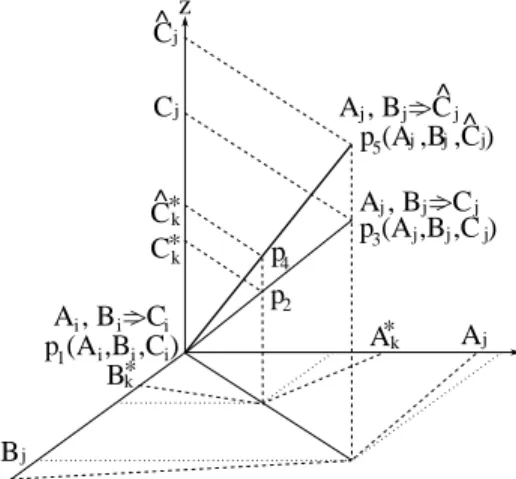
Although AFRI is applicable to fuzzy inference problems with multiple-antecedent rules, for illustrative simplicity, rules with two antecedents are taken in this work as an example to show the underlying approach. The method can be extended to rules with more than two antecedent variables in a straight-forward manner. Given an input (A∗k, Bk∗), suppose that the (closest) neighbouring rules Ai, Bi ⇒ Ci andAj, Bj ⇒Cj
flank this input. Without losing generality, assume that the second rule is defective and is included in the candidate to be modified, and that(Ai, Bi)is less than(Aj, Bj)in accordance with the integration of their representative values (for a given integration method). Based on the location of the antecedent of this defective rule, in reference to the other rule that was jointly fired with it to derive the detected contradictory interpolated result, two mirrored cases need to be addressed.
First, consider the case where the location relation between the input (A∗k, Bk∗), and its corresponding interpolated conse-quence Ck∗ is mapped by the line P1P3 within the assumed three dimensional space, as shown in Fig. 5. This line is determined by the locations of the two neighbouring rules used for interpolation. Suppose that the defective rule consequence is modified from Cj to Cjb , then the original mapping line
P1P3is accordingly shifted to the lineP1P5. To quantitatively measure the extent of such shifting, the following correction rate c− is introduced:
c−= d(Ci,Cbj)
d(Ci, Cj), (24) whered(C, C′)stands for the distance between the fuzzy sets
CandC′, computed as the distance between the representative values of these two fuzzy sets. Suppose that the modified result ofCk∗ is denoted asCbk∗. Then, by applying the correction rate
c− to the distance between Ci andCk∗, the distance fromCi
to Cbk∗ can be determined. Having known the locations ofCi
andCk∗, the location ofCbk∗ can be computed, resulting in the modified interpolated value.
The case discussed above covers the case where an input which has invoked the defective rule for interpolation is less than the integrated antecedent of the rule. For the case where an input is greater than the antecedent, a mirrored procedure is followed to perform the modification, with a different
correction ratec+. Assume that the input(A∗
k, B∗k)is flanked
by the defective ruleAi, Bi⇒Ci and the other neighbouring rule, Aj, Bj ⇒Cj, thenc+ is defined as:
c+=d(Ci, Cjb )
d(Ci, Cj). (25) The modified result of (A∗k, Bk∗)can then be calculated using this correction rate, in a way similar to that utilised in the first case. A , B = Ci i i> x y z p (A ,B ,C ) p (A ,B ,C ) p (A ,B ,C ) p p A , B = Cj j j> j j j j j j 1 2 3 4 5 k Aj B C C A B i i i j k j j * * C k * ^ ^ ^ ^ A , B = Cj j j> C k *
Fig. 5. Propagation of rule modification
C. Modification of Both Neighbouring Rules
Having addressed the situations where only one of the two neighbouring rules appears in a candidate for modification, this sub-section discusses the modification of both neighbouring rules which are defective (i.e., both are included in a given candidate).
Suppose that the two defective neighbouring rules are
Ai, Bi ⇒ Ci and Aj, Bj ⇒ Cj, and denote the (to be) modified consequences of them as Cib and Cjb , respectively. For easy reference, call the defective rule whose integrated antecedent is less than the input the left rule and the other the right. If the left rule is modified first as illustrated in Fig. 6(a), then the right defective rule will be modified using the result of modifying the left rule, as shown in Fig. 6(b). Then, the final modification can be represented by shifting the original defective location mapping lineP1P3to the lineP6P5
as also illustrated in Fig. 6(b). If, however, the modification begins with the right defective rule, the modification will be performed as illustrated in Fig. 7, which also results in the final result that is the same as the one represented by the lineP6P5
in Fig. 6(b). From this, due to the generality in the expression of the two rules, it can be concluded that the revised result is independent of the order of modifications. Therefore, the modification of both neighbouring rules in a single candidate can be done by revising the two individual defective rules separately in either order.
D. Illustrative Example - Part 2
Continue the example given in Sec. III-F, the candidateC1,
which is of the highest priority, will be modified first. As only one modifiable elementR3 (Ifx2=B3, THENx3=C3) is
contained in this candidate, the modification procedure given in Section IV-B is applied. With respect to Eqs. 15 and 16, the modification of the defective rule,R3 needs to satisfy:
b C3≥C3−1−20.6(20−0) b C3≤C3+1−20.6(20−0) min(supp(Cb3))≥0 max(supp(C3b ))≤20.
A , B = Ci i i> x y z p (A ,B ,C ) p (A ,B ,C ) p p j j j 1 2 3 4 k Aj B C A B i i i j k j * * C k * A , B = Ci i i> p (A ,B ,C )6 i i i ^ ^ ^ A , B = Cj j j> C k * ’
(a) Left rule modification first
A , B = Ci i i> x y z p (A ,B ,C ) p (A ,B ,C ) p (A ,B ,C ) p p A , B = Cj j j> j j j j j j 1 2 3 4 5 k Aj B C A B i i i j k j C*k * * C k * ^ ^ ^ ^ A , B = Ci i i> p (A ,B ,C )6 i i i ^ ^ ^ p7 A , B = Cj j j> C k * ’
(b) Right rule modification second Fig. 6. Rule modification starting from left defective rule
Running interpolation with the two neighbouring rules con-sisting of the rule R4 and the defective one R3 leads to the following two interpolated rules:
IR1: IF x2 isB∗, THENx3 isC2∗ IR2: IF x2 isB∗1, THENx3 isC1∗.
Since both antecedents of IR1 andIR2 are greater than the
antecedent of the defective rule,C+ is applied: c+=d(Cb3, C4)
d(C3, C4).
From this, the overall location of the modified results will then
satisfy: {
d(Cb1∗, C4) =d(C1∗, C4)·c+ d(Cb2∗, C4) =d(C2∗, C4)·c+.
These results are then utilised to further constrain the modified interpolated values such that
{ b
C1∗=C1∗+ (d(Cb1∗, C4)−d(C1∗, C4)) b
C2∗=C2∗+ (d(Cb2∗, C4)−d(C2∗, C4)).
The remaining process of the modification is to ensure that the modified results and their propagations are consistent with
A , B = Ci i i> x y z p (A ,B ,C ) p (A ,B ,C ) p (A ,B ,C ) p p A , B = Cj j j> j j j j j j 1 2 3 4 5 k Aj B C C A B i i i j k j j * * C k * ^ ^ ^ ^ A , B = Cj j j> C k * ’
(a) Right rule modification first
A , B = Ci i i> x y z p (A ,B ,C ) p (A ,B ,C ) p (A ,B ,C ) p p A , B = Cj j j> j j j j j j 1 2 3 4 5 k Aj B C A B i i i j k j C*k * * C k * ^ ^ ^ ^ A , B = Ci i i> p (A ,B ,C )6 i i i ^ ^ ^ p 7 A , B = Cj j j> C k * ’
(b) Left rule modification second Fig. 7. Rule modification starting from right defective rule
the rest. This sub-process is again, the same as that of the modification of a FIC as previously reported [24]. However, by solving all the simultaneous equalities and inequalities as listed above, including those imposed by the consistency-ensuring sub-process, there is no solution found. Therefore, the candidate with the second highest priority, that is C2 in
this example, is modified next.
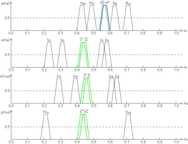
The candidate C2 includes two elements, the observation O2and the ruleR8, both of which need to be modified
simul-taneously in order to remove inconsistency. The modifications ofO2andR8are carried out based on the procedures given in Sections IV-A and IV-B, respectively. In particular, according to constraint number 1 of the observation modification process, the modified value ofO2 must satisfy:
b B∗≥B∗−1−0.6 2 (20−0) b B∗≤B∗+1−20.6(20−0) min(supp(Bb∗))≥0 max(supp(Bb∗))≤20.
Similar constraints are also applied to the modified result of the consequence of R8. As the modification procedure of
R8 is the same as that ofR3, as described above, the compu-tational details are omitted here. By solving the equalities and
inequalities, including those posed for consistency-ensuring, one solution is obtained as illustrated in Fig. 8. With the consistency restored, this concludes this illustrative example.
Fig. 8. One solution of the running example
E. Computational Complexity
As the generalisation of AFRI, it may be expected that the generalised AFRI will involve more computation than its original. In particular, as compared to the computational complexity of AFRI, that of the generalised version can be considered from the following two viewpoints:
• Impact of adding rules and observations as diagnosable candidate elements during candidate generation;
• Impact of the constraints led by these extra candidate elements during candidate modification.
The computational complexity of candidate generation mainly depends on the complexity of the ATMS. It is well known that the standard ATMS has a computational complexity of exponential order in the worst case [41], but the average-case complexity can be greatly improved during practice use [42], [43]. The introduction of observations and rules as diagnosable candidate elements certainly increases the processing time because of a more sophisticated problem is being addressed. However, this does not affect the general time complexity of the underlying ATMS. The complexity of the candidate modification stage is mainly determined by the constraint sat-isfaction mechanism which for the problem of FRI in general, can be resolved in polynomial time complexity [24]. Although the introduction of additional constraints may increase the
absolute computing time, the general time complexity will not be affected as the constraints introduced by the extra modifiable candidate elements are of the same type with those used in AFRI. Putting both aspects together, at the system level, the overall computational complexity of the generalised version does not deteriorate from that of the original AFRI approach.
V. APPLICATION ANDDISCUSSION
Disease burden may result from environmental changes [44]–[46]. An example study of this concerns how a previously roadless area in northern coastal Ecuador may be affected by the construction of a new road or railway in term of epidemiology of infectious diseases [47]. The causal relationship between the key factors driven by road construction has been established in the work of [47], which has been further quantitatively investigated using AFRI in [24]. As the theoretical development reported in this paper carries a substantial extension of [24], the application problem is reconsidered in this paper to facilitate direct comparison. For completeness, the sparse rule base is given below and the fuzzy values included in the rules are listed in Table I.
R1: IFx1=A1 andx2=B1, THENx3=C1 (0.9); R2: IFx1=A2 andx2=B2, THENx3=C2 (0.9); R3: IFx3=C3 andx4=D3, THENx5=E3 (0.7); R4: IFx3=C4 andx4=D4, THENx5=E4 (0.8); R5: IFx5=E5, THENx6=F5 (0.8); R6: IFx5=E6, THENx6=F6 (0.6); R7: IFx6=F7, THENx7=G7 (0.7); R8: IFx6=F8, THENx7=G8 (0.7); R9: IFx5=E9, THENx8=H9 (0.8); R10: IFx5=E10, THENx8=H10 (0.6); R11: IFx8=H11, THENx9=I11 (0.7); R12: IFx8=H12, THENx9=I12 (0.9); R13: IFx9=I13, THENx10=J13 (0.7); R14: IFx9=I14, THENx10=J14 (0.8); R15: IFx7=G15 andx10=J15, THENx11=K15 (0.6); R16: IFx7=G16 andx10=J16, THENx11=K16 (0.8). Suppose that four pieces of uncertain information are ob-served: O1 : x1 = A∗ = (0.16,0.18, 0.20,0.22)(0.7), O2 : x2 = B∗ = (0.34,0.36,0.38,0.40)(0.9), O4 : x4 = D∗ = (0.65,0.67,0.69, 0.71)(0.6), and O8 : x8 = H∗ =
(0.54,0.56,0.58,0.60)(0.7). These observations do not invoke any rule in the rule base (with only B∗ overlapping with the second antecedent attribute B2 of the rule R2). Thus, traditional fuzzy system techniques that are based on the use of compositional rule of inference cannot be employed to address the problem. However, fuzzy rule interpolation may help.
Assume that the set-theory-based similarity measure is utilised to compute the degree of contradiction, and letβ0=
0.5. β0-contradictions will result from most of the existing
interpolation methods [24]. In particular, the interpolated result using the scale and move transformation-based FRI, which the proposed work is built upon, leads to multiple (indeterminate)
β0-inconsistencies as shown in Fig. 9.
To obtain a consistent solution, the proposed adaptive fuzzy interpolation approach is applied. From the modifiable com-ponents (i.e., observations, rules and FICs) upon which the