Financial Vulnerability

299

F

inancial

v

ulnerability

Marcelo Fuenzalida

Jaime Ruiz-Tagle

Department of Economics, Universidad de Chile

Household indebtedness in Chile has received considerable attention in recent years because of the financial deepening process underway in the economy. Although various macroeconomic indicators show significant increases in the last decade, there are few tools for evaluating the real vulnerability of this sector from a financial stability perspective. One of these tools is stress testing using microeconomic information.

Although households may face a variety of financial risks from a range of sources, the household sector is most sensitive to changes in household income, such as those caused by unemployment (Debelle, 2004a, 2004b). Moreover, household vulnerability to aggregate shocks that raise the unemployment rate will depend on both debt distribution and household characteristics. The heterogeneity of indebtedness levels and income uncertainty calls for microeconomic analysis.

The main objective of this paper is to carry out a household stress test at the microeconomic level that allows quantifying household debt at risk when facing aggregate shocks. Evidence from debt issuers indicates that the main reason for households to default is unemployment, so we focus on labor income risk associated with the At the time of writing, Marcelo Fuenzalida was affiliated with the Central Bank of Chile.

We thank Dante Contreras, Kevin Cowan, and Eric Parrado for useful comments. Ruiz-Tagle also acknowledges financial support from the Central Bank of Chile and from the Iniciativa Científica Milenio of the Centro de Microdatos at the Universidad de Chile (Project P07S-023-F).

Financial Stability, Monetary Policy, and Central Banking, edited by Rodrigo A. Alfaro, Santiago, Chile. © 2010 Central Bank of Chile.

probability of job loss when the aggregate unemployment rate shifts. For this purpose, we use panel data survival analysis to estimate the probability of job loss at the individual level. We then run Monte Carlo simulations to assess household financial stress by estimating aggregate debt at risk under high unemployment rate scenarios.

Financial data at the household level are scarce, which is one of the reasons why there are so few household-level studies assessing household financial indebtedness. The recent Chilean Household Financial Survey (EFH) carried out by the Central Bank of Chile contributes novel information for this type of analysis.

Nordic countries have been leading this sort of analysis The Swedish Central Bank has published a series of simulations based on microeconomic data.1 _{They find that Swedish households are not}

particularly vulnerable to shifts in interest rates or unemployment rates. Specifically, 6.3 percent of households have what they call a negative margin, accounting for 5.6 percent of total household debt (debt at risk). Unemployment rate increases of 1–3 percentage points cause the share of households without a margin to rise to 6.7 percent and debt at risk to 6.3 percent. Vatne (2006) carries out a similar exercise, finding that 19 percent of households have a negative margin and that they account for 16 percent of total debt. The study concludes that low and median income groups hold the majority of the exposed debt and have increased their share over time.

Neither study, however, takes into account that aggregate unemployment does not have a uniform impact on agents across households. In fact, they consider that the probability of falling into unemployment is uniform for all workers. This is a very strong assumption and can bias the results depending on the distribution of debt among individuals. In Chile, there is evidence that unemployment is less frequent within high education groups and among middle-aged workers (Neilson and Ruiz-Tagle, 2007), supporting heterogeneous responses.

The remainder of the paper is organized as follows. Section 1 analyses the distribution of household indebtedness in Chile and discusses debt at risk using data from the 2007 Household Financial Survey. Section 2 estimates job loss probabilities based on data from the Social Protection Survey Panel, covering a ten-year period from 1995 to 2004. Nonparametric and semiparametric methods are used to 1. See Johansson and Persson (2006) and Gyntelberg, Johansson, and Persson (2007).

estimate the impact of aggregate unemployment rates on individual job loss probabilities. Section 3 carries out simulations of debt at risk under different scenarios. For this purpose, job loss probabilities are imputed into the EFH data, and then Monte Carlo simulations are run to assess the distribution of the stress test. Finally, section 4 concludes.

1. h

i

D

R

Household borrowing has grown considerably in Chile, both in absolute terms and relative to household income. In fact, the growth rate of debt has consistently surpassed that of real GDP over the last decades. This has raised concerns about the household sector’s vulnerability and possible implications for the stability of the financial system. Households’ ability to pay back debts and the amount of debt they hold determine how much of this debt could be considered at risk of not being recovered by credit issuers.

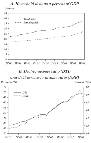
Bank debt represents more than 70 percent of total household debt (see figure 1) and grew almost 15 percent, on average, in real annual terms between 2003 and 2008. Real bank debt thus almost doubled during this period, while real GDP increased almost 30 percent. Moreover, the growth of total household debt surpassed the growth of households’ disposable income, causing the debt-to-disposable-income ratio to grow significantly over the last several years. In the fourth quarter of 2008, this aggregate indicator reached almost 69 percent, from 44 percent in the fourth quarter of 2003. Furthermore, the ratio of the household financial burden to disposable income also expanded, rising from 14 percent to 20 percent in the same period (figure 1).

Since bank debt is by far the most important household debt, the financial system’s exposure to the household sector is a matter of concern from a financial stability perspective. Bank exposure, measured as the share of total mortgage and consumer loans in total bank loans, increased from 15 percent at the beginning of the 1990s to more than 33 percent in 2008.

Although Chilean households are increasing their debt, the trend in Chile is not significantly different from other countries. In fact, the relationship between household debt to GDP and per capita GDP suggests that household debt is not a significant share of GDP. Nevertheless, the financial-burden-to-disposable-income ratio is not particularly low given the country’s economic development, measured as per capita GDP (see figure 2). This last observation

Figure 1. Chilean Household Indebtedness at the Macroeconomic Level

A. Household debt as a percent of GDP

B. Debt-to-income ratio (DTI) and debt-service-to-income ratio (DSR)

Source: Central Bank of Chile.

is related to the length of the loans and the high interest rates, relative to developed economies.2

Microeconomic analysis reveals an important heterogeneity among Chilean households. In particular, the vast majority of debt is held by high-income groups. This is particularly important in 2. There is a caveat about the financial burden. In some countries, debt service refers only to interest payments, while others (including Chile) define it to include both interest and principal payments.

Chile because of the high levels of income inequality. In fact, debt distribution maps rather well with income distribution.

Different microeconomic surveys find a similar pattern, though it may be changing slightly over time, suggesting a financial deepening process (see figure 3; see also figure A1 in the appendix). Moreover, households’ behavior in terms of their ability to pay back debts may vary considerably depending on their debt and income levels. This is an important reason to consider household heterogeneity when analyzing household financial vulnerability.

Figure 2. Household Debt: International Comparison

A. Household debt and economic developmenta

B. DSR and household debt

Source: IMF Global Financial Stability Report 2006.

a. The countries inside the circle are Argentina, Brazil, China, Colombia, India, Indonesia, Peru, Philippines, Romania, Russia, Turkey, and Venezuela.

Figure 3. Chilean Household Indebtedness at the Microeconomic Level

A. Distribution of debt by income quintile: 2007 EFH

B. DSR by income quintile

Source: Authors’ calculations, based on data from the 2004 EPS, 2006 CASEN, and 2007 EFH.

In the remainder of this section, we describe our data sets and discuss the debt-at-risk methodology used.

1.1 The Chilean Household Financial Survey

Assessing household financial vulnerability requires detailed financial data at the household level. The recent Chilean Household Financial Survey (Encuesta Financiera de Hogares, or EFH), contributes with novel information for this type of analysis.

The EFH was conducted by the Central Bank of Chile for the first time in 2007. This survey includes detailed questions about labor status, real estate ownership, financial assets, debt, perceptions of debt service, access to credit, pensions, insurance, and savings. The 2007 EFH covered 4,021 households and was representative at the national urban level. Furthermore, since a small fraction of the population holds a large share of assets, the survey oversampled wealthier households. This skew in the sample was possible thanks to the collaboration of the Chilean Internal Revenue Service. The 2007 EFH thus constitutes the only statistical source in Chile that provides complete information on household balance sheets and their ability to service financial commitments.3

1.2 Debt Distribution and Debt at Risk

There is no common definition of debt at risk. The Central Bank of Chile uses a definition based on the ratio of debt service over income (that is, the debt service ratio, or DSR).4 _{Norway and Sweden}

consider negative margins (that is, when total spending exceeds total income). They also include liquid and illiquid assets as debt backup. For household h, the margin is computed as

M_h = Y_h - DS_h - E_h, (1)

where Y_h is total household income, DS_h is debt service, and E_h is total household expenditures.

In this paper, the baseline scenario of debt at risk is built considering two dimensions: a negative financial margin and a high DSR. Data collection posses two problems for interpretation. First, there is a risk of double counting. For example, clothing expenditures could also appear as debt if purchased with a credit card. Second, if

3. For a description of the 2007 Chilean Household Financial Survey and a discussion of the methodology and results, see Central Bank of Chile (2009).

a significant share of total expenditures is made with credit cards (including supermarket expenditures, for example), the DSR indicator could actually overestimate the financial stress of the households.

Taking into account these caveats, we build our baseline scenario for debt at risk considering both a negative financial margin and a high DSR. The negative financial margin is set at 20 percent excess expenditure over income, and the DSR is considered high when it is above 50 and above 75. Table 2 presents results for the baseline scenario of debt at risk based on the debt service ratio and the financial margin. The table reveals that 13.6 percent of households exhibit a negative margin and a DSR larger than 50 percent, accounting for 20 percent of total debt. A more refined assessment of debt at risk, with the DSR above 75 percent, indicates that 9.5 percent of households are highly financial stressed and 16 percent of total debt is at risk (15 percent of secured debt and 19 percent of unsecured debt).

2. a

f

v

Household financial vulnerability in Chile is mainly due to income sources, since only a negligible share of household debt has a variable interest rate. Households’ main income source is the labor income of their members.5 _{Labor income can be lost if the job ends for any}

reason, whether voluntary or involuntary. At any time, workers face a given probability of losing their jobs. By imputing these job loss probabilities to working individuals, we can assess their financial vulnerability, provided the financial information is available. However, there are no available estimates of job loss probabilities in Chile.6

This section therefore provides estimates of job loss probabilities based on survival analysis using nonparametric and semiparametric methods. In particular, the interest is focused on the effect of aggregate unemployment rate on job loss probabilities.

The effects of aggregate unemployment are heterogeneous in both a static and dynamic framework. Given that the distribution of household debt is diverse, the impact of higher unemployment levels generates nonhomogeneous effects on debt at risk. The Norwegian and Swedish studies propose a simplified analysis assuming that unemployment

5. Neilson and others (2008) document that labor dynamics is the main factor driving entry and exit from income-stressing conditions. In the EFH, labor income accounts for more than 60 percent of total households income.

shocks affect all individuals in the same manner. Although limited, that methodology makes sense for them because the distribution of debt in those countries is much flatter than in Chile (particularly in Norway), and also because they have large unemployment benefits that cover a substantial part of lost income for a long period. In contrast, for Chile it is more appropriate to estimate disaggregated job loss probabilities to assess heterogeneous impacts.

2.1 Job Loss Probability

Estimating job loss probabilities requires survival analysis. In this case, job loss probability mirrors the probability of staying employed. What is estimated, then, is the probability of remaining employed (or surviving, in the analysis) at a given moment of time t.

Let T be a nonnegative random variable denoting the time to failure (in this case, failure is job loss). The survival function is the reverse of the cumulative distribution function of T[F(t)]:

S(t) = 1 -F(t) = Pr(T> t). (2)

It reports the probability of surviving beyond time t, where the density function is simply f(t) = -S'(t).

The cumulative hazard function is defined as

H(t) = -ln[S(t)], (3)

such that

f(t) = h(t)exp[-H(t)]. (4)

For the purpose of this paper, what is interesting is how some covariates affect the hazard function, which requires multivariate analysis. Nevertheless, simpler nonparametric analysis can be used to compare different groups’ hazard functions. This is done by estimating the survival function through the Kaplan-Meier (1958) estimator, given by ˆ _, | S t n d n j j j j t tj ( )=  -       ≤

∏

where n_j is the number of individuals at risk at time t_j and d_j is the number of failures at time t_j.

The Cox (1972) semiparametric model requires no parametric form of the survival function. It assumes that covariates shift multiplicatively the baseline hazard function. For the jth subject, the hazard function is:

h t( Xj t,)=h t0( )exp(Xj t x,β ), (6)

where Xj,t is a vector of variables, and the values of βx are estimated

from the data.

The baseline function h₀(t) is not parameterized (or even estimated), because the model is proposed in terms of ratios (individual j compared with individual m):

h t h t j t m t j t x m t x ( ) ( ) exp( ) exp( ) , , , , X X X X = β β . (7)

The Cox model is rather convenient for the purpose of this paper, because it is easy to compute and can provide predicted probabilities given the covariates.

Parametric methods require imposing a functional form to the baseline hazard function. The most common are the Weibull, exponential, lognormal, gamma and log-logistic models. These models are computationally costly, and they also have the disadvantage of bias in case of an inappropriate distributional assumption.

This papers combines different nonparametric, semiparametric, and parametric methods to accurately predict job loss probabilities.

2.2 The Data

The Social Protection Survey (Encuesta de Protección Social, EPS) has been carried out in Chile every two years since 2002. This panel survey was designed to assess the well-being of workers and nonworkers and their households.7 _{The EPS includes 16,727 observations,}

representing the population of Chile aged 18 and over in 2004.

7. The EPS was designed jointly by the Ministry of Labor and the Centro de Microdatos of the Universidad de Chile, with the close collaboration of the University of Pennsylvania.

In the 2002 wave, the individuals were asked to chronologically list every single labor experience since 1980. Each experience had a beginning date and an ending date. For each experience, the individuals were asked about their employment status, the characteristics of the job, and some qualitative questions. In the 2004 wave, individuals were asked to provide the missing history, that is, the experiences that occurred between 2002 and 2004.

The data are then organized into a monthly panel of individuals with the corresponding employment information in each period. This gives us the employment status of a sample that is representative of the Chilean population aged 18 and more in 2004. Representativeness in past years narrows to a varying age group. For instance, in 2004 the data are representative of people between 18 and 65 years old, in 2003, between 18 and 64 years old, and so on.

In this paper, we use a ten-year period from 1995 to 2004. This period comprises the Asian crisis and a relatively short mild recession in 1999 and 2000. Consequently, the unemployment rate rose significantly and remained high for a long period afterward. Given this timeframe, the sample covers 16,727 individuals over 120 months, which implies that the data set has around two million records.

2.3 Estimation Results

We estimate job loss probabilities using the labor experiences reported in the 2002 and 2004 EPS. The probabilities incorporate a set of individual characteristics, X_jt, and a set of time variant aggregate variables, Z_jt. The X_jt vector of variables includes gender, age, education, job contract, marital status, economic sector of the job, and size of the firm. The Z_jt vector considers the aggregate unemployment rate and monthly activity indexes.

We define job loss as any exit from a job resulting in unemployment of inactivity. This definition reflects our objective of assessing households’ ability to cope with their financial obligations, since any decay in income will increase household financial stress.

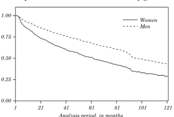
To assess survival heterogeneity, we first look at the Kaplan-Meier nonparametric estimates of the survival functions. Figure 4 presents estimates of the survival function by gender and educational level. Men are less likely to lose employment than women at any time: the mean estimator indicates that men remain employed 50 percent longer than women, and the probability of losing employment reaches 50 percent only after 80 months for both genders. Workers with tertiary

Figure 4. Job Loss Probabilities

A. Kaplan-Meier survival estimates by gender

B. Kaplan-Meier survival estimates by education level

Source: Authors’ calculations, based on data from the 2002 and 2004 EPS.

education have a much lower probability of losing employment than those with primary and secondary education. Workers with secondary education have a larger job loss probability than those with primary education at shorter employment durations and a lower job loss probability after 90 months.

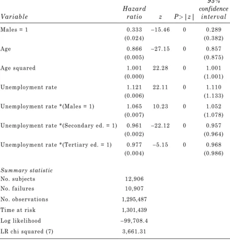
Next, we carried out multivariate analysis for multiple specifications using the Cox semiparametric estimates of the proportional hazard model. Table 1 presents our preferred model. A series of interesting results emerge from the data. First, the job loss probability of men is around 30 percent lower probability than women. The unemployment rate shifts that probability by 17 percent,

Table 1. Cox Estimations of Job Loss Probabilities

Variable Hazard ratio z P>|z|

95% confidence interval Males = 1 0.333 –15.46 0 0.289 (0.024) (0.382) Age 0.866 –27.15 0 0.857 (0.005) (0.875) Age squared 1.001 22.28 0 1.001 (0.000) (1.001) Unemployment rate 1.121 22.11 0 1.110 (0.006) (1.133)

Unemployment rate *(Males = 1) 1.065 10.23 0 1.052

(0.007) (1.078)

Unemployment rate *(Secondary ed. = 1) 0.961 –22.12 0 0.957

(0.002) (0.964)

Unemployment rate *(Tertiary ed. = 1) 0.977 –5.15 0 0.968

(0.004) (0.986) Summary statistic No. subjects 12,906 No. failures 10,907 No. observations 1,295,487 Time at risk 1,301,439 Log likelihood –99,708.4 LR chi squared (7) 3,661.31

Source: Authors’ calculations.

a. Coefficients are in exp(β) form. Standard errors are in parentheses.

but it seems to have a much larger effect on men than women (around 8 percent per unemployment percentage point).

Second, age has a decreasing negative effect on job loss probabilities. This means that younger workers are much more likely to lose employment at any given time than older workers, but the effect fades as age increases.

Third, workers with higher levels of education face a significantly lower probability of losing their jobs. Those with tertiary education have about a 30 percent lower probability than those with

primary education only. The effect of the unemployment rate is also heterogeneous among different education groups. Workers with tertiary education have a 5 percent lower probability per unemployment percentage point (implying about 45 percent lower probability, on average) than those with primary education only. Workers with secondary education face a 3 percent lower probability per unemployment percentage point (implying about 27 percent lower probability on average) than those with primary education only.

From the Cox estimates, we can predict job loss probabilities through the survival functions. Figures 5 and 6 show the survival function estimates for women and men, respectively. Age was set at mean values (around 41 years old), and unemployment shifts were set at 10 percent, 15 percent, and 20 percent. It is clear from the graphs that higher educational attainment diminishes job loss probabilities and, more importantly for our purposes, also diminishes the impact of an aggregate unemployment shift. Women exhibit higher probabilities of job loss (the survival functions are lower), but aggregate unemployment shifts affect men considerably more than women.

A. Survival function: Women with primary education

B. Survival function: Women with secondary education

C. Survival function: Women with tertiary education

A. Survival function: Men with primary education

B. Survival function: Men with secondary education

C. Survival function: Men with tertiary education

3. f

s

s

This section is devoted to the analysis of higher unemployment rates simulations and their effects on debt at risk. We ran Monte Carlo simulations on the probability of losing employment for each of the worker individuals in each household. We then imputed the employment loss probabilities determined earlier to the EFH data set.

The first problem for this exercise is that the EFH does not contain information about employment duration. Employment loss probabilities depend critically on the duration of the job, so we had to impute employment duration. To do so, we separated workers into cells by age group and educational attainment. For each cell, the whole distribution of employment duration was computed as ˆdc.

Then, every worker j in cell c was assigned a random employment duration following the actual distribution dc ~ ˆ . Hence, this is the dc

first source of randomization.8

We then ran the simulations as follows. First, we assigned a uniform random number u_jh to each worker in the EFH. For each worker in the EFH with an assigned employment duration dc with

characteristics X_jh and under the scenario given by Zt_{, we computed}

a job loss probability using the estimated parameters from the hazard function. If that probability is below the threshold given by the random number, the worker is considered to be employed. If not, the worker is considered to have lost his or her employment, so labor income in this case becomes zero.

ˆ _{ˆPr ( , ) .}

Yjht =Yjht ×1_ jht X Ztjh t >u_ (8)

The second source of randomization comes from the fact that the simulated employment loss probability contains the uncertainty with respect to the survival model estimate through the probability of losing the job.

After the worker’s employment condition of the worker is redefined and the corresponding labor income recomputed, overall household income is computed again. The DSR must also be refreshed to reflect the simulated total household income. Finally, aggregate indicators of debt at risk are computed again for the whole sample.

8. For the simulations, the actual cumulative density function, Φdˆc, was approximated by a nine-degree polynomial. Figures A2 and A3 in the appendix show those estimates.

In the baseline scenario, 61 percent of total households hold some sort of formal debt. Specifically, 16 percent of households hold secure debt, and 57 percent hold unsecured debt. Secure debt is 60 percent of total debt (unsecured debt is 40 percent). Moreover, 45 percent of total debt is held by the upper richest quintile (51 percent of secure debt and 36 percent of unsecured debt). The median DSR is 19.5 percent for all indebted households.

Table 2 presents the results of the simulations.9 _{In the baseline}

scenario, with the DSR above 75 percent and the negative margin above 20 percent, 9.5 percent of households are considered to have debt at risk. Those households accounts for 16.1 percent of total household debt.

We then use the underlying job loss probabilities to expand the current debt at risk to include households whose members could lose their jobs at any moment, thus falling into higher financial stress. This raises the number of households under financial stress to between 13 percent and 16 percent, while total debt at risk increases to between 20 percent and 25 percent, with a 95 percent confidence interval.10

Next, we increase the unemployment rate by 5 percent. This is a larger increase than occurred during the Asian crisis. Under this scenario, the number of households under high financial stress increases to between 16 percent and 19 percent, and debt at risk rises to between 22 percent and 28 percent. A 15 percent increase in unemployment increases the number of highly stressed households to between 25 percent and 28 percent, and debt at risk to between 31 percent and 38 percent. These results indicate that significant increases in the aggregate unemployment rate do not necessarily imply a significant increase in debt at risk relative to the current situation.

These results imply that higher levels of unemployment, similar to what was observed during the Asian crisis, do not necessarily generate a significant household default shock in the financial system. In this scenario, debt at risk only increases around 4 percentage points (compared with the baseline scenario including underlying job loss probabilities). Nevertheless, this 9. We used 500 Monte Carlo simulations. Exercises with 1,000 and 5,000 simulations did not produce significantly different results.

10. We built the 95 percent confidence intervals nonparametrically using simulation percentiles.

Table 2. Households with a Negative Margin

Scenario

and DSR threshold Households Secured debt Unsecured debt Total debt

Baseline scenario

DSR > 50 13.6 17.1 26.1 20.2

DSR > 75 9.5 14.5 18.8 16.1

Baseline scenario

+ underlying job loss probability

DSR > 50 18.2 – 20.8 20.3 – 26.3 30.8 – 36.5 24.3 – 29.4 DSR > 75 13.2 – 15.6 17.1 – 22.6 23.1 – 29.0 19.7 – 24.6 Delta+ 5% unemployment DSR > 50 21.5 – 24.4 22.9 – 30.2 34.1 – 40.4 27.1 – 33.0 DSR > 75 15.9 – 18.8 19.2 – 26.2 26.2 – 33.3 22.3 – 28.1 Delta+ 10% unemployment DSR > 50 26.1 – 29.5 26.7 – 35.3 38.7 – 45.6 31.2 – 38.3 DSR > 75 20.1 – 23.3 22.8 – 30.2 30.9 – 38.8 25.9 – 32.6 Delta+ 15% unemployment DSR > 50 31.0 – 34.6 31.9 – 40.9 44.3 – 51.4 36.6 – 44.3 DSR > 75 24.5 – 28.0 27.0 – 35.3 36.4 – 44.3 31.0 – 37.9

Source: Authors’ calculations.

a. The intervals for the simulations are p(2.5) to p(97.5), and are given in percent.

does not mean that the financial system can overlook household debt. Table 2 suggests that for a one-percentage-point increase in the unemployment rate, debt at risk expands between 0.6 and 0.8 percentage points.11

The DSR threshold of 75 percent is not very demanding for considering a household under high financial stress. Table 2 includes a 50 percent threshold, and figure 7 complements the analysis by presenting a range of DSR thresholds under an unemployment shift of 5 percent and with the negative margin at 1.2. The results are fairly stable, with no extreme shifts in debt at risk.12

11. Jappelli, Pagano, and di Maggio (2008) study a sample of eleven member countries of the European Union. They estimate 0.37 percentage points increase in arrears for each percentage point increase in the unemployment rate.

Figure 7. Debt at Risk Simulations at Different DSR Thresholdsa

A. Households with debt at risk B. Secured debt at risk

C. Unsecured debt at risk D. Total debt at risk

Source: Authors’ calculations.

a. Unemployment shift of 5 percent and a negative margin of 1.2.

We also look at the distribution of the effects by income quintiles. Figure 8 presents the baseline scenario plus the extreme scenarios (percentiles 2.5 and 97.5) under a 5 percent increase in the aggregate unemployment rate. When unemployment increases, debt at risk will only increase significantly if the households in the high income quintiles are affected. Our estimates of the job loss probabilities indicate that this is fairly unlikely under all circumstances. However, the bottom line is that income, high-debt households should be monitored.

A. Baseline scenario

B. Scenario: 5 percent increase in unemployment, p(2.5)

C. Scenario: 5 percent increase in unemployment, p(97.5)

Finally, several issues are not considered in this simulation exercise. First, as workers face nonnegative unemployment probabilities, unemployed (and inactive) workers face a nonnegative probability of becoming employed and then being able to contribute labor income to household financial resources. Second, workers who lose their jobs may have unemployment insurance, although in Chile this does not imply a significant source of income.13 _Third,

workers who retire to inactivity may have pension income. Fourth, households that experience unemployment may use other sources of income to face their financial obligations, making default less likely to occur. Fifth, households that experience unemployment may sell assets in order to avoid default. Finally, since household-level default data are not available, the increase in debt at risk after a shock should be interpreted as household debt that could come under financial strain, rather than an increase in nonperforming loans. All these caveats go in the same direction, which is to make this simulation exercise less stressing for households’ financial situation. Consequently, this exercise should be considered as an upper bound that is unlikely to occur.

4. C

The indebtedness of the household sector has increased significantly in recent years in Chile. However, no analysis had been carried out previously to assess how vulnerable households could be in terms of their financial stress under aggregate unemployment shifts. This paper contributes with a novel analysis aimed at quantifying the associated risks for financial stability.

Households display significant heterogeneity in terms of the fragility of their main income source, labor income, implying that microeconomic studies must be used to assess aggregate impacts of unemployment on financial stress. Gender, age, and education are the key factors that determine the size of the impact of unemployment shocks on the probability of losing a job.

We find that for a one-percentage-point increase in the unemployment rate, debt at risk increases between 0.6 and 0.8 percentage points. However, because household debt is concentrated in high income households, heterogeneous responses to unemployment may have important implications for financial stability. In fact, the

13. Unemployment insurance covers 30 percent of earnings for three months for a worker who has been employed at least 40 consecutive months.

simulations carried out on the different shock scenarios show that debt at risk is rather bounded.

Higher levels of unemployment do not necessarily generate a significant household default shock in the financial system. Nevertheless, this does not mean that the financial system can overlook household debt.

a

Supplemental Figures

Figure A1. Distribution of Chilean Household Indebtedness by Income Quintile

A. Based on the 2004 EPS

B. Based on the 2006 CASEN

A. Women aged 18–24 B. Women aged 25–34

C. Women aged 35–44 D. Women aged 45–54

E. Women aged 55–65

A. Men aged 18–24 B. Men aged 25–34

C. Men aged 35–44 D. Men aged 45–54

E. Men aged 55–65

A. Households with debt at risk B. Secured debt at risk

C. Unsecured debt at risk D. Total debt at risk

Source: Authors’ calculations based on 2002 and 2004 EPS. a. Unemployment shift of 5 percent and a negative margin of 1.1.

R

Central Bank of Chile. 2009. “Encuesta financiera de hogares: EFH 2007 metodología y principales resultados.” Santiago.

Cox, D.R. 1972. “Regression Models and Life-Tables (with discussion).”

Journal of the Royal Statistics Society Series B 34: 187–220. Cox, P., E. Parrado, and J. Ruiz-Tagle. 2006. “The Distribution

of Assets, Debt, and Income among Chilean Households.” In

Proceedings of the IFC Conference on “Measuring the Financial

Position of the Household Sector,” Basel, 30–31 August 2006, vol.

2. IFC bulletin 26. Basel: Bank for International Settlements. Debelle, G. 2004a. “Household Debt and the Macroeconomy.” BIS

Quarterly Review (March).

. 2004b. “Macroeconomic Implications of Rising Household Debt.” Working paper 153. Basel: Bank for International Settlements.

Gyntelberg, J., M.W. Johansson, and M. Persson. 2007. “Using Housing Finance Micro Data to Assess Financial Stability Risks.”

Housing Finance International 22(1): 3–8.

Jappelli, T., M. Pagano, and M. di Maggio. 2008. “Households’ Indebtedness and Financial Fragility.” Working paper 208. University of Naples, Centre for Studies in Economics and Finance (CSEF).

Johansson, M. and M. Persson. 2006. “Swedish Households’ Indebtedness and Ability to Pay: A Household Level Study.”

Sveriges Riksbank Economic Review 2006(3): 24–41.

Kaplan, E.L. and P. Meier. 1958. “Nonparametric Estimation from Incomplete Observations.” Journal of the American Statistical

Association 53: 457–81.

Neilson, C., D. Contreras, R. Cooper, and J. Hermann. 2008. “The Dynamics of Poverty in Chile.” Journal of Latin American Studies

40: 251–73.

Neilson, C. and J. Ruiz-Tagle. 2007. “Worker Flows and Labor Dynamics in Chile: A Retrospective Story.” University of Chile. Vatne, B.H. 2006. “How Large are the Financial Margins of

Norwegian Households? An Analysis of Micro Data for the Period 1987–2004.” Norges Bank. Economic Bulletin 4/06: 173–80.