MONETARY CONSERVATISM AND FISCAL POLICY
Klaus Adam and Roberto M. Billi
First version: September 29, 2004
This version: February 2007
RWP 07-01
Abstract:
Does an inflation conservative central bank à la Rogoff (1985) remain
desirable in a setting with endogenous fiscal policy? To provide an answer we study
monetary and fiscal policy games without commitment in a dynamic stochastic sticky
price economy with monopolistic distortions. Monetary policy determines nominal
interest rates and fiscal policy provides public goods generating private utility. We find
that lack of fiscal commitment gives rise to excessive public spending. The optimal
inflation rate internalizing this distortion is positive, but lack of monetary commitment
robustly generates too much inflation. A conservative monetary authority thus remains
desirable. When fiscal policy is determined before monetary policy each period, the
monetary authority should focus exclusively on stabilizing inflation, as this eliminates the
steady state biases associated with lack of monetary and fiscal commitment. It also leads
to stabilization policy that is close to if not fully optimal.
Keywords
: sequential non-cooperative policy games, discretionary policy, time consistent
policy, conservative monetary policy
JEL classification
: E52, E62, E63
We thank Marina Azzimonti, Helge Berger, V.V. Chari, Gauti Eggertsson, Jordi Galí,
Albert Marcet, Ramon Marimon, seminar participants at IGIER/Bocconi University,
participants at the Third Conference of the International Research Forum on Monetary
Policy and the 11th International Conference on Computing in Economics and Finance
for helpful comments and discussions. Errors remain ours. The views expressed herein
are solely those of the authors and do not necessarily reflect the views of the European
Central Bank, the Federal Reserve Bank of Kansas City or the Federal Reserve System.
Affiliations: Adam, European Central Bank, Kaiserstr. 29, 60311 Frankfurt, Germany;
Center for Economic Policy Research (CEPR), London; Billi, Federal Reserve Bank of
Kansas City, 925 Grand Blvd, Kansas City, MO 64198, United States.
1
Introduction
The di!culties associated with executing optimal but time-inconsistent policy plans have received much attention following the seminal work of Kydland and Prescott (1977) and Barro and Gordon (1983). Time inconsistency problems, however, have hardly been analyzed in a dynamic setting where monetary and fiscal policymakers are separate authorities engaged in a non-cooperative policy game. This may appear surprising given that the institutional setup in most developed countries suggests such an analysis to be of relevance.
In this paper we analyze non-cooperative monetary and fiscal policy games assuming that policymakers cannot commit to future policy choices. We start by identifying the policy biases emerging from sequential and non-cooperative decision making and show how these biases interact with each other. We then provide a normative analysis assessing the implications of installing a central bank that is conservative in the sense of Rogo(1985).1 In other terms, we
an-alyze the desirability of central bank conservatism in a setting with endogenous fiscal policy.
Presented is a dynamic stochastic general equilibrium model without capi-tal, along the lines of Rotemberg (1982) and Woodford (2003), featuring three sources of distortions: (1) the presence of monopolistically competitive firms, which cause equilibrium output to be ine!ciently low; (2) rigidities to price adjustment, which give rise to real eects of monetary policy; (3) policymakers than cannot credibly commit to a path for future policy, but instead determine policy sequentially, i.e., at the time of implementation.
In line with recent monetary policy models, we consider a monetary author-ity determining the short-term nominal interest rate. We add to this a fiscal authority deciding about the level of public goods provision. Public goods gen-erate utility for private agents and are financed by lump sum taxes, so as to balance the government’s intertemporal budget.
While all policymakers are assumed benevolent, i.e., they maximize the util-ity of the representative agent, lack of commitment gives rise to suboptimal policy outcomes. In particular, since output is ine!ciently low, both policy-makers are tempted to increase output, either via lowering real interest rates (monetary authority) or via increasing public spending (fiscal authority). Com-pared to a situation with policy commitment, this results in an inflationary bias and in overspending on public goods. The ine!ciency arises because both poli-cymakers fail to fully internalize the welfare cost of generating inflation today. The presence of nominal rigidities requires price setters to be forward-looking, i.e., their price setting decisions depend positively on expected future inflation. Policymakers that decide sequentially fail to perceive the implications of their 1Walsh (1995) and Svensson (1997) discuss alternative institutional arrangements for
current policy decisions on pricing decisions in the past, since past prices can be taken as given at the time policy is determined. As a result, sequentially deciding policymakers underestimate the welfare costs of generating inflation today and are tempted to move output closer to its first-best level.
In our setting monetary and fiscal policy interact in interesting ways. In particular, taking the lack of fiscal commitment as given, it becomes optimal for monetary policy to implement positive inflation rates.2 We show that positive
inflation rates reduce the fiscal spending bias and thereby increase agents’ utility. This suggests that - unlike in the standard case with exogenous fiscal policy - a conservative central bank may not be desirable. Yet, a quantitative assessment suggests that the optimal deviations from price stability tend to be small. And more importantly, in the non-cooperative Markov-perfect Nash equilibrium with sequential monetary and fiscal policy, the steady state inflation rate lies above the optimal inflation rate for a wide range of model parameterizations.3 This suggests that installing an inflation conservative central bank remains desirable with endogenous fiscal policy.
We then formally introduce a conservative central bank that maximizes a weighted sum of an inflation loss term and the representative agent’s utility. And we characterize the resulting Markov-perfect equilibria.
For the case where policies are determined simultaneously or the case where monetary policy is determined before fiscal policy each period, it fails to be possible to eliminate entirely the steady state distortions via monetary conser-vatism alone. There is either positive inflation or fiscal overspending or both. Nevertheless, we find that an appropriate degree of monetary conservatism is desirable, as it eliminates most of the steady state welfare losses arising from the lack of monetary and fiscal commitment.
Monetary conservatism is even more desirable if fiscal policy is determined before monetary policy each period (arguably the most relevant timing proto-col). In such a setting monetary conservatism is internalized by fiscal policy and this makes it possible to reduce the inflation bias as well as the public spending bias. In particular, a monetary authority that cares exclusively about stabiliz-ing inflation allows to recover the Ramsey steady state, i.e., fully eliminates the biases stemming from lack of monetary and fiscal commitment. The case for a conservative central bank may thus appear even stronger once endogenous fiscal policy is considered.
We also briefly address the issue of how the conduct of stabilization policy is aected by the presence of a conservative central bank. In particular, we 2In our setting, a monetary authority controlling nominal interest ratesUhas full control
over the steady state inflation rate, as it has to satisfyU=31, where denotes the
discount factor. See equation (9).
3Markov-perfect Nash equilibria, as defined in Maskin and Tirole (2001), are a standard
show that fiscal leadership in combination with a fully conservative central bank allows to implement the flexible price Ramsey policy response to technology and mark-up shocks. This suggests that monetary conservatism has also desirable stabilization properties.
The remainder of this paper is structured as follows. After discussing the re-lated literature in section 2, section 3 introduces the economic model and derives the implementability constraints characterizing private sector behavior. Section 4 considers monetary and fiscal policy with and without commitment, derives analytical results about the policy biases resulting from lack of commitment, and discusses how these biases interact with each other. In section 5 we provide a quantitative assessment of the steady state eects generated by sequential monetary and fiscal policymaking. Section 6 introduces a conservative central bank and analyzes the welfare gains associated with monetary conservatism. A conclusion briefly summarizes the results and provides an outlook for future work. Technical material is contained in the appendix.
2
Related Literature
Problems of optimal monetary and fiscal policy are traditionally studied within the optimal taxation framework introduced by Frank Ramsey (1927). In the so-called Ramsey literature, monetary and fiscal authorities are treated as a ‘single’ authority and decisions are taken at time zero, e.g., Chari and Kehoe (1999).4 In seminal contributions, Kydland and Prescott (1977) and Barro and Gordon (1983) show that time zero optimal choices might be time-inconsistent, i.e., reoptimization in successive periods would imply a dierent policy to be optimal than the one initially envisaged.
The monetary policy literature has extensively studied time-inconsistency problems in dynamic settings and potential solutions to it, e.g., Rogo(1985), Svensson (1997) and Walsh (1995). However, in this literature fiscal policy is typically absent or assumed exogenous to the model. Similarly, a number of contributions analyze sequential fiscal decisions and the time-consistency of optimal fiscal plans in dynamic general equilibrium models, e.g., Lucas and Stokey (1983), Chari and Kehoe (1990) or Klein, Krusell, and Ríos-Rull (2006). This literature typically studies models without money.
An important strand of the literature, developed by Sargent and Wallace (1981), Leeper (1991), and Woodford (2001), studies monetary and fiscal policy interactions using policy rules, e.g., Schmitt-Grohé and Uribe (2007) and Ferrero (2005). This literature, however, does not consider time-inconsistency problems, as it assumes policymakers to be fully committed to simple rules.
4Galí and Monacelli (2005) extend the Ramsey approach to the case of a monetary union,
A range of papers discusses monetary and fiscal policy interactions with and without commitment in a static framework where monetary and fiscal policy-makers interact only once, e.g., Alesina and Tabellini (1987). This paper goes beyond these earlier contributions by studying a fully dynamic and stochastic model where current economic outcomes are influenced also by expectations about the future. This is similar in spirit to a recent paper by Díaz-Giménez et al. (2006) which determines sequential optimal policy in a fully dynamic cash-in-advance economy with government debt. While they study a flexible price model in which interactions between monetary and fiscal policy operate through seigniorage and the government budget constraint, we abstract from seigniorage as a source of government revenue. Instead, we focus on the interactions arising from the presence of nominal rigidities.
3
The Economy
In the next sections we first introduce a sticky-price economy model, similar to the one studied in Schmitt-Grohé and Uribe (2004), then we derive the private sector equilibrium for dierent monetary and fiscal policy regimes.
3.1
Private Sector
There is a continuum of identical households with preferences given by
H0 4 X w=0 wx(f w> kw> jw) (1)
where fw denotes consumption of an aggregate consumption good, kw 5 [0>1]
labor eort,jwpublic goods provision by the government in the form of aggregate
consumption goods, and5(0>1)the subjective discount factor. Throughout the paper we assume:
Condition 1 x(f> k> j) is separable in f> k>and j. Moreover, xf A0,xff?0, xk?0,xkk0,xj A0,xjj ?0, and¯¯¯fxxfff ¯¯¯,¯¯¯kxxkkk¯¯¯are bounded for (f> k> j)5
[0>1]×[0>1]×[0>1].
Each household produces a dierentiated intermediate good. Demand for this intermediate good is given by
|wg à e Sw Sw !
where|wdenotes (private and public) demand for the aggregate good,Sewis the
nominal price of the good produced by the household, and Sw is the nominal
price of the aggregate good. The demand functiong(·)satisfies
g(1) = 1 g0(1) =w
where w5 (4>1) is the price elasticity of demand for the dierent goods.
This elasticity is assumed to be time-varying and induces fluctuations in the mo-nopolistic mark-up charged by firms. The assumed demand function is consis-tent with optimizing individual behavior when private and public consumption goods are a Dixit-Stiglitz aggregate of the goods produced by dierent house-holds.5 The household chooses Se
w, then hires the necessary amount of labor
eortekwto satisfy the resulting product demand, i.e., }wkew=|wg à e Sw Sw ! (2) where}wdenotes an aggregate technology shock. We assume the mark-up shock
and the technology shock to follow AR(1) stochastic processes, respectively,
w=(1) +w1+%w }w= (1}) +}}w1+%}w
where ?1 denotes the steady value of the price elasticity of demand, and the innovations%lw(l=> })are mean zero, independent both across time and
cross-sectionally, with small bounded support.
Following Rotemberg (1982), we describe sluggish nominal price adjustment by assuming that firms face quadratic resource costs for adjusting prices accord-ing to 2 Ã e Sw e Sw1 1 !2
where A0measures the degree of price stickiness. The flow budget constraint of the household is given by
Swfw+Ew=Uw1Ew1+Sw 5 7Sew Sw |wgw à e Sw Sw ! zwekw2 à e Sw e Sw1 1 !26 8+SwzwkwSwow (3) whereUwis the gross nominal interest rate,Ewdenotes nominal bonds that pay UwEw in periodw+ 1, zw is the real wage paid in a competitive labor market,
andoware lump sum taxes.
Although bonds are the only available financial instrument, assuming com-plete financial markets instead would make no dierence for the analysis, since households have identical incomes in a symmetric price setting equilibrium. One should note that we abstract from money holdings. This can be inter-preted as the ‘cashless limit’ of a model economy with money, see Woodford
5That is| w U l |l w 1+w w di w 1+w where|l
w denotes the input of the good produced by householdl.
(1998). Money thus imposes only a lower bound on the nominal interest rate, i.e.,Uw1, each period.6
Finally, we impose a no-Ponzi scheme borrowing constraint on household behavior lim m$4Hw w+Ym1 l=0 1 Ul Ew+m0 (4)
that has to hold each period and at all contingencies.
The household’s problem consists of choosing {fw> kw>ekw>Sew> Ew}4w=0 so as to maximize (1) subject to (2), (3) and (4) taking as given {|w> Sw> zw> Uw> jw> ow}4w=0. Using equation (2) to substituteekw in (3) and letting the multiplier on (3) be
w
Sw, the first order conditions of the household’s problem are then equations (2),
(3) and (4) holding with equality and also
xfw=w xkw xfw =zw (5) w Uw =Hw w+1 w+1 0 =w |wg(uw) +uw|wg0(uw) zw }w |wg0(uw) μ w uw uw1 1 ¶ w uw1 ¸ +Hww+1 μ uw+1 uw w+11 ¶ uw+1 u2w w+1
whereuw SShww denotes the relative price andw SSww1 is the gross consumer
price inflation rate. Furthermore, there is the transversality condition
lim
m$4Hw
w+mxfw+mEw+m Sw+m
= 0 (6)
which has to hold each period and at all contingencies.
3.2
Government
The government consists of two authorities, i.e., a monetary authority setting short-term nominal interest rates and a fiscal authority deciding on government expenditures and lump sum taxes.
6Abstracting from money entails that we ignore possible seigniorage revenues generated in
the presence of positive nominal interest rates. Since we allow for lump sum taxes, one can safely ignore the fiscal implications of such revenues.
Government expenditures consist of spending related to the provision of public goods jw and socially wasteful expenditure { that does not generate
utility for private agents. The level of public goods provision jw is a choice
variable, while{is taken to be exogenous. The government’s budget constraint is then given by
Ew=Uw1Ew1+Sw(jw+{ow) (7)
The availability of lump sum taxesowimplies that decisions regarding tax versus
debt financing do not matter for equilibrium determination. Ricardian equiva-lence applies as long as the implied paths for the debt level satisfy the no-Ponzi scheme borrowing constraint (4) and the transversality condition (6) at all con-tingencies. For sake of simplicity, we assume taxes to be set such that the level of real debtEw
Sw remains bounded from below and asymptotically grows at a rate
less than 1. Constraints (4) and (6) are then always satisfied and can be ignored from now on. Fiscal policy is thus ‘passive’ in the sense of Leeper (1991).
Note that equation (7) assumes government purchases are subject to the same monopoly mark-up as purchases by consumers. Assuming instead the government faces a dierent mark-up would not aect the resulting equilibrium allocations. The availability of lump sum taxes allows the government to raise additional income without generating distortions; profit income from sales to the government and taxes exactly oset each other in the households’ budget constraint.
3.3
Private Sector Equilibrium
In a symmetric price setting equilibrium the relative price is given byuw = 1
for all w. From the assumptions made in the previous section, it follows that the first order conditions of households behavior can be condensed into a price setting equation xfw(w1)w= xfw}wkw μ 1 +w+ xkw xfw w }w ¶ +Hwxfw+1(w+11)w+1 (8)
often referred to as a ‘Phillips curve’, and a consumption Euler equation
xfw Uw
=Hw xfw+1
w+1 (9)
A private sector rational expectations equilibrium is then a set of plans
{fw> kw> Ew> Sw} satisfying equations (8) and (9), the government budget
con-straint (7), and the market-clearing condition
}wkw=fw+
2(w1)2+jw+{ (10)
given the policies{jw> ow> Uw1}, the value of{, the exogenous stochastic processes
3.4
Time Inconsistency Problems
Under commitment policymakers determine the entire state-contingent sequence of future policies at the beginning of time. Instead, if policymakers cannot com-mit to future policy plans, they decide about policies at the time of implemen-tation, i.e., period by period. We refer to such behavior as sequential decision making. As we argue below, sequential policy leads to suboptimal outcomes.
Consider the price setting equation (8). As can be seen, firms’ profit max-imizing rate of price increase in periodw is a function of the expected rate of price increase fromwtow+1. Policymakers’ actions in periodw+ 1will influence the equilibrium price level inw+ 1, but from the perspective of periodw+ 1the prices in periodwcan be taken as given. Therefore, policymakers that determine policies in periodw+ 1 will fail to incorporate the impact of their policy deci-sions on periodw inflation rates. Yet, the private sector rationally anticipates the policy decisions in periodw+ 1. From the perspective of periodw, sequential decision making in periodw+ 1is therefore suboptimal.
Sequentially deciding policymakers fail to take fully into account the welfare implications of their policy choices. In the present setting, policymakers will underestimate the welfare costs of generating inflation today.
4
Monetary and Fiscal Policy Regimes
In this section we study the outcomes associated with dierent degrees of com-mitment in monetary and fiscal policy. The main focus in on the steady state implications of the dierent policy regimes. Consideration of the responses to mark-up and productivity shocks is deferred to section 6.
It turns out useful to start by analyzing the first-best allocation, i.e., the allocation that would be achieved in the absence of monopoly distortions and nominal rigidities. In a second step we consider the Ramsey allocation, which takes into account both distortions, but assumes commitment to policies at time zero. In a final step we relax the assumption of policy commitment.
4.1
First-Best Allocation
The first-best allocation solves
max {fw>kwjw} H0 4 X w=0 wx(fw> kw> jw) s.t. }wkw=fw+jw+{ (11)
where equation (11) is the resource constraint. The steady state first-order conditions deliver
showing, as expected, that it is optimal to equate the marginal utility of private and public consumption to the marginal disutility of labor eort. The next section shows that this ceases to be optimal once monopoly and price setting distortions are taken into account.
4.2
Ramsey Policy
Assuming commitment to policies at time zero and full cooperation between monetary and fiscal policymakers, the Ramsey allocation solves7
max {fw>kw>w>Uw1>jw} H0 4 X w=0 wx(fw> kw> jw) (12) s.t.
Equations (8)>(9)>(10)for allw
The Ramsey planner maximizes the utility function of the representative agent subject to the implementability constraints (8) and (9), which summarize the price setting and monopoly distortion in the economy, the feasibility constraint (10), and the lower bound on nominal interest rates.8 As shown in appendix
A.1, the Ramsey steady state is characterized by
= 1
U= 1
the feasibility constraint (10) and the marginal conditions
xf = 1 +xk (13) xj = 1 + 1+t 1 +t xk (14) wheret f kkxxkkk xf
fxff 0. Equation (13) shows that monopolistic competition
creates a wedge between the marginal utility of private consumption and the marginal disutility of work. This reflects the fact that labor fails to receive its marginal product when firms have monopoly power, which causes housholds to reduce consumption of produced goods and to increase consumption of leisure.9
7Since Ricardian equivalence holds we ignore the financing decisions of the fiscal authority
and the initial debt levelU31E31, which do not matter for equilibrium determination of the other variables. Since the initial conditionS31simply normalizes the implied price level path, it can equally be ignored.
8In what follows, we abstract from the non stationary component of time zero optimal
policies. In our numerical application we ascertain that the time zero commitment policies asymptotically approach the steady states values reported below and also verify that the non stationary component does not alter the welfare conclusions.
9From equations (5) and (13), it follows thatz=1+
?1in steady state, i.e., real wages fall short of their marginal product.
Forxkk?0, one hast A0and equation (14) implies that the optimal level of
public spending falls short of equating the marginal utility of public consumption to the marginal disutility of work, unlike in the first best allocation. At first, one might think that the optimal provision of public goods should not be aected by the presence of a monopolistic mark-up, since the availability of lump sum taxes implies that the government can finance the price mark-up without generating additional distortions. Yet, reduced public spending also reduces the marginal disutility of work and thereby helps to increase the ine!ciently low level of private consumption. To see how, note that reducing government spending and lump sum taxation correspondingly has no wealth eects on households, as household income and taxes are reduced by exactly the same amount. Reducing spending and taxes, therefore, aects the households’ problem only via a reduced marginal disutility of work.
4.3
Sequential Policymaking
We now consider separate monetary and fiscal authorities that cannot commit to future policy plans, instead they decide policies at the time of implemen-tation, i.e., period-by-period. To facilitate the exposition, we assume that a sequentially deciding policymaker takes as given the current policy choice of the other policymaker as well as all future policies and future private sector choices. We prove the rationality of this assumption at the end of this section.
4.3.1 Sequential Fiscal Policy
Consider sequential fiscal policymaking. Given the assumptions made above, the fiscal authority’s problem in periodwis
max {fw+m>kw+m>w+m>jw+m} Hw 4 X m=0 mx(fw+m> kw+m> jw+m) (15) s.t.
Equations (8)>(9)>(10)for allw
{fw+m> kw+m>w+m> Uw+m11> jw+m} given form1
As shown in appendix A.2, the first order conditions associated with problem (15) deliver the fiscal reaction function
xjw= xkw }w 2w1 2w1(w1) (1 +w+xxkwfw}ww +kwxxkkwfw }ww) (FRF) where the fiscal authority sets the level of public goods provision jwsuch that
FRF is satisfied, each period.
Consider a steady state in which = 1, i.e., with an inflation rate equal to the one chosen by the Ramsey planner. The fiscal reaction function then simplifies to
showing that fiscal policy equates the marginal utility of public consumption to the marginal disutility of labor eort. While such behavior is consistent with the first-best allocation, it is generally suboptimal in the presence of monopolis-tic distortions, see the discussion in section 4.2. Sequential fiscal policy implies a suboptimally high level of public spending, i.e., a ‘fiscal spending bias’. This spending bias causes the Ramsey allocation to be unattainable in the presence of sequential fiscal policy, because either inflation, fiscal spending, or both must deviate from their Ramsey values. This is summarized in the following propo-sition.
Proposition 1 For xkk ? 0, sequential fiscal policy implies excessive fiscal spending in the presence of price stability.
The economic intuition underlying this result is as follows. By taking future decisions and the current monetary policy choiceUwas given, the fiscal authority
considers private consumption fw to be determined by the Euler equation (9).
Given this, the fiscal authority perceives labor inputkwto move one-for-one with
government spendingjw. In a situation with price stability, the inflation costs
of public spending are zero (at the margin) and can be ignored. This causes the sequential spending rule (16) to appear optimal. In the general case6= 1, the marginal costs of inflation fail to be zero, leading to the more general expression given in FRF.
4.3.2 Sequential Monetary Policy
We now consider sequential monetary policy. Given the assumptions made above, the monetary authority’s problem in periodw is
max {fw+m>kw+m>w+m>Uw+m1} Hw 4 X m=0 mx(fw+m> kw+m> jw+m) (17) s.t.
Equations (8),(9),(10) for allw
{fw+m> kw+m>w+m> Uw+m1> jw+m1} given form1
As shown in appendix A.3, the first order conditions associated with problem (17) deliver the monetary reaction function
}wxfw xkw (w(w1)w)(w1)w μ 1 +kwxkkw xkw ¶ + 2w1 xffw xfw (w1) ((w1)w}wkw(1 +w)) = 0 (MRF)
where the monetary authority sets the nominal interest rateUwsuch that MRF
is satisfied, each period. Appendix A.4 proves the following result.
Proposition 2 Forsu!ciently close to 1, sequential monetary policy implies a strictly positive rate of inflation in steady state.
Sequential monetary policy thus generates an inflation bias as in the stan-dard case with exogenous fiscal policy, e.g., Svensson (1997). Intuitively, the monetary authority is tempted to stimulate demand by lowering nominal inter-est rates. Since price adjustments are costly, the price level will not fully adjust, real interest rates fall, stimulating demand. The real wage increase required to satisfy this additional demand generates inflation, but the welfare costs of inflation are not fully taken into account for reasons discussed before.
4.3.3 Sequential Monetary and Fiscal Policy
We now define a Markov-perfect Nash equilibrium with sequential monetary and fiscal policy. We start by verifying the rationality of our initial assumption that a sequentially deciding policymaker can take as given the current policy choice of the other policymaker, as well as all future policies and future private sector decisions.
The private sector’s optimality conditions (8) and (9), the feasibility con-straint (10), as well as the policy reactions functions (FRF) and (MRF), all depend on current and future variables only. This suggests the existence of an equilibrium where current play is a function of the current exogenous vari-ables}w and w only. Future play then depends on future exogenous variables
only, thereby justifying the assumption that future equilibrium play (and o -equilibrium play) is independent of current play. If each period, in addition, monetary and fiscal policy are determined simultaneously, Nash equilibrium re-quires taking the other players’ current decisions as given. This justifies the assumptions made in deriving (FRF) and (MRF) and motivates the following definition.
Definition 3 (SP) A stationary Markov-perfect Nash equilibrium with sequen-tial monetary and fiscal policy consists of time-invariant policy functionsf(}w> w)> k(}w> w)> (}w> w)> U(}w> w)> j(}w> w)solving equations (8),(9),(10), (FRF) and (MRF).
We now show that assuming Stackelberg leadership by one of the policy authorities, instead of simultaneous decision making, does not aect the equi-librium outcome. While the policy problem of the Stackelberg follower remains unchanged, the Stackelberg leader should take into account the reaction func-tion of the follower. Importantly, however, the Lagrange multipliers associated with additionally imposing either MRF in the sequential fiscal problem (15) or FRF in the sequential monetary problem (17) are zero. In fact, these reaction functions can be derived from the first order conditions of the leader’s policy problem even when the follower’s reaction function is not being imposed.
Intuitively, the leadership structure does not matter for the equilibrium out-come because the monetary and fiscal authorities are pursuing the same policy objective. Any departure of the equilibrium outcome from the Ramsey solution
is thus entirely due to the assumption of sequential decision making. However, the presence of dierent policymakers and the sequence of moves will matter in section 6 when we consider a monetary authority that is more inflation averse than the fiscal authority.
4.4
Monetary and Fiscal Policy Interactions
This section analyzes how the fiscal spending bias and agents’ utility is aected by the steady state inflation rate. Since steady state inflation depends on steady state nominal interest rates only, see equation (9), we implicitly analyze how the conduct of monetary policy aects fiscal policy and welfare. Appendix A.5 derives the following result.
Proposition 4 Assume xkk ? 0. In a steady state with sequential fiscal pol-icy, agents’ utility increases and fiscal spending decreases with the steady state inflation rate, locally at= 1.
The previous proposition implies that price stability ceases to be optimal once fiscal policy fails to commit to its spending plans and is described by FRF. Intuitively, inflation increases the perceived costs of public spending for the fiscal authority, thereby reduces the fiscal spending bias. This makes it optimal to implement positive inflation rates.
The optimal inflation rate that appropriately internalizes the sequential fiscal policy distortion is obtained as a solution to the following problem10
max {fw>kw>w>Uw1>jw} H0 4 X w=0 wx(fw> kw> jw) (OI) s.t.
Equations (8),(9),(10),(FRF) for allw
Here we assume that monetary policy can commit, but fiscal behavior is de-scribed by FRF. We will refer to this situation as the optimal inflation (OI) regime. If the optimal inflation rate is lower (higher) than the inflation bias generated in a Markov-perfect Nash equilibrium with sequential monetary and fiscal policy, an inflation conservative (liberal) central bank would appear desir-able. Whether the optimal inflation rate is above or below the inflation bias is ultimately a quantitative issue. We address it in the next section.
5
Quantitative Evaluation of Policy Biases
In this section we explore the quantitative importance of relaxing the assump-tion of monetary and fiscal policy commitment. In particular, we quantify the 1 0As before, we abstract from non-stationary components of time zero optimal policies in
welfare implications associated with the presence of steady state biases in in-flation and public spending. In addition, we compare the steady state outcome under sequential policy (SP) to that achieved under the optimal inflation (OI) regime.
5.1
Parameterization
We assume the following preference specification, which satisfies condition 1 and is consistent with balanced growth,
x(fw> kw> jw) = log (fw)$k k1+w *
1 +*+$jlog (jw) (18)
with$kA0,$j 0and *0denoting the inverse of the Frisch labor supply
elasticity.
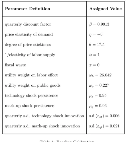
The baseline calibration of the model is summarized in table 1. The quarterly discount factoris chosen to match the average ex-post U.S. real interest rate during the period 1983:1-2002:4, i.e.,3=5%. The steady state value for the price elasticity of demand is set at 6, implying a mark-up over marginal cost of 20%. The degree of price stickiness is chosen to be 17=5, such that the log-linearized version of the Phillips curve (8) is consistent with the estimates of Sbordone (2002), as in Schmitt-Grohé and Uribe (2004). The elasticity of labor eort is assumed to be one (*= 1) and we abstract from wasteful fiscal spending, i.e.,{= 0. The utility weights$kand$j are chosen such that in the
Ramsey steady state agents work 20% of their time(k= 0=2)and spend 20% of output on public goods (j= 0=04).11 The process for the technology shock }
w
is taken from Schmitt-Grohé and Uribe (2004).12 The parameterization for the mark-up shock processwis taken from Ireland (2004).13
To test the robustness of our results, we consider also a wide range of alter-native model parameterizations. For comparability, the utility weights$k and $j are adjusted so as to leave the Ramsey steady state unchanged.
The actual computational method we employ to numerically solve for the Markov-perfect Nash equilibrium with sequential monetary and fiscal policy is described in appendix A.7. A useful by-product of this approach is that it delivers second-order accurate welfare expressions for economies with a distorted steady state, while relying on linear-quadratic approximation only.
1 1The values of$
kand$jare set according to equations (47) and (48), respectively, derived in appendix A.6.
1 2To transform the annual values reported in table 1 of Schmitt-Grohé and Uribe (2004),
we raise the AR-coe!cient of the technology shock to the power 1/4 and divide the standard deviation of the shock innovation by 4.
1 3Table 1 in Ireland (2004) presents estimates for the scaled mark-up shock process w . Multiplying his estimate for the standard deviation by our price adjustment cost= 17=5
yields the standard deviation in our table 1. Ireland’s estimate for the technology shock process is similar to the one used in this paper.
5.2
Steady State Implications
Employing the baseline calibration summarized in table 1, we now investigate the quantitative impact of relaxing monetary and fiscal policy commitment. In addition, we compare the outcome under sequential policy (SP) to that achieved under the optimal inflation (OI) regime. Finally, we analyze the robustness of the quantitative findings to dierent model parameterizations.
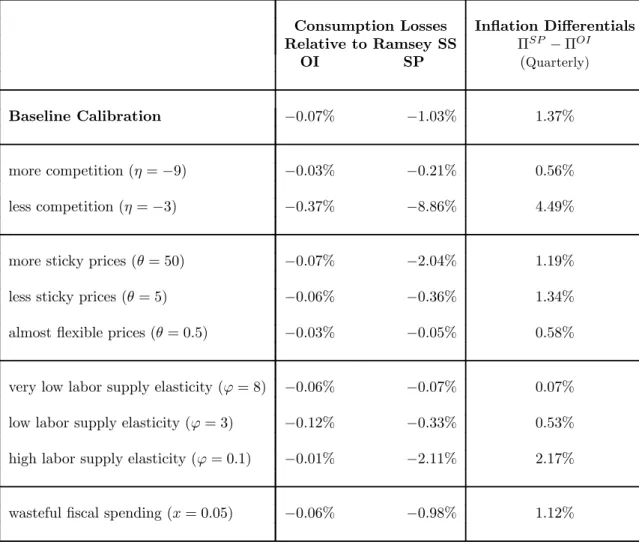
The first row of table 2 presents information on the steady state in the SP regime. All variables are expressed as percentage deviations from their corre-sponding Ramsey steady state values.14 The last column of the table reports the steady state welfare loss, expressed in terms of the permanent reduction in private consumption that would imply the Ramsey steady state to be welfare equivalent to the considered policy regime.15 In line with proposition 2, the sequential policy outcome is characterized by an inflation bias, which turns out to be sizable. In addition, there is a small fiscal spending bias. Overall, the welfare losses generated by the sequential conduct of policy are fairly large, in the order of 1% of steady state consumption per period.
The second row of table 2 shows the outcome under the OI regime. The optimal inflation rate turns out to be not only lower than the one in the SP regime but also very close to the Ramsey value. Note that reducing inflation from the level of the SP regime to the optimal level increases the fiscal spending bias, as suggested by proposition 4. While the fiscal spending increase associated with reduced inflation is fairly large, implementing the optimal inflation rate nevertheless eliminates large part of the welfare losses associated with the SP regime. This suggests that the fiscal spending bias, despite being sizable in absolute value, is not very detrimental in welfare terms. Clearly, this result hinges partly on the assumed availability of lump sum taxes.
The results from table 2 suggest that - for the particular parameterization considered thus far - installing a conservative monetary authority is desirable in a situation where lack of fiscal commitment is described by FRF. The op-timal inflation rate is well below the one emerging in the SP regime. Also, a conservative monetary authority may eliminate large part of the welfare losses associated with sequential monetary and fiscal policymaking.
Table 3 explores the robustness of the previous findings to a wide range of changes in the model parameterization.16 The table reports the steady state
welfare losses associated with the dierent policy regimes in the middle column and suggests that the previous findings are robust. In particular, significant
1 4In the Ramsey steady statef= 0=16,k= 0=2,j= 0=04and= 1. 1 5Appendix A.8 explains how to compute these welfare losses. 1 6For all parametrizations considered in table 3, the utility weights$
kand$jare adjusted to leave the Ramsey steady state unchanged. When considering wasteful fiscal expenditure
welfare gains can be realized from implementing the optimal inflation rate. Ex-ceptions are the flexible price limit($0) and the cases with inelastic labor supply (large values for*). For these cases the time-inconsistency problems of monetary and fiscal policy disappear and real allocations approach the Ramsey steady state under SP. Table 3 also reports the dierence between inflation in the SP regime and the optimal inflation rate (right column). For all parame-terizations the optimal inflation rate (OI) is below the one emerging in the SP regime. This suggests an inflation conservative monetary authority to be desir-able in all these settings, provided FRF describes fiscal behavior. We investigate this issue in detail in the next section.
6
Conservative Monetary Authority
This section analyzes whether the distortions stemming from sequential mone-tary and fiscal policy decisions can be reduced by installing a central bank that is more inflation averse than society. Rogo (1985) and Svensson (1997) have shown this to be the case if fiscal policy is treated as exogenous.
Following Rogo (1985), we consider a ‘weight conservative’ monetary au-thority with period utility function
(1)x(fw+m> kw+m> jw+m)
(w1)2
2
where5[0>1] is a measure of monetary conservatism. For A0the mone-tary authority dislikes inflation (and deflation) more than society; if= 1the policymaker cares about inflation only. The preferences of the fiscal authority remain unchanged.
With monetary and fiscal authorities now pursuing dierent policy objec-tives, the equilibrium outcome will depend on the timing of policy moves, i.e., on whether fiscal policy is determined before, after, or simultaneously with monetary policy each period. Casual observation suggests that it takes longer to enact fiscal decisions, which would imply that fiscal policy is determined before monetary policy. At the same time, the time lag between a monetary policy decision and its eects on the economy may also be substantial. It thus remains to be ascertained, which of these timing structures is the most relevant for actual economies. For these reasons, we consider Nash as well as leadership equilibria.
6.1
Nash and Leadership Equilibria
This section defines the various Markov-perfect equilibria in the presence of a conservative monetary authority. As will be clarified below, with simultaneous monetary and fiscal decisions (Nash case) and with monetary policy determined before fiscal policy (monetary leadership), sequential fiscal behavior remains
described by FRF, i.e., by the reaction function in the absence of a conservative central bank. This diers from the situation where fiscal policy is determined before monetary policy (fiscal leadership), because the fiscal authority takes into account the conservative monetary authority’s reaction function. Monetary policy can then use ‘o-equilibrium’ behavior to discipline the behavior of the fiscal authority along the equilibrium path. Fiscal leadership thus opens the possibility for outcomes that are welfare superior to those achieved in the OI regime.
First, consider the case with simultaneous decisions. While the policy prob-lem of the fiscal authority remains unchanged, the monetary authority now solves max {fw+m>kw+m>w+m>Uw+m1} Hw 4 X m=0 m³(1)x(fw+m> kw+m> jw+m) 2(w1)2 ´ (19) s.t.
Equations (8),(9),(10) for allw
{fw+m> kw+m>w+m> Uw+m1> jw+m1} given form1
As shown in appendix A.9, the first order conditions associated with problem (19) deliver the conservative monetary authority’s reaction function
}wxfw xkw (w(w1)w)(w1)w μ 1 +kwxkkw xkw ¶ + 2w1xffw xfw (w1) ((w1)w}wkw(1 +w)) ¸(1)}w xkw (1)+x1 fw = 0 (CMRF) For= 0, CMRF reduces to the monetary reaction function without conser-vatism (MRF).17 This motivates the following definition.
Definition 5 (CSP-Nash) A stationary Markov-perfect Nash equilibrium with sequential and conservative monetary policy, sequential fiscal policy and simul-taneous policy decisions consists of policy functionsf(}w> w)> k(}w> w)>(}w> w)> U(}w> w)> j(}w> w)solving equations (8), (9), (10), (FRF) and (CMRF).
Next, we consider the case of monetary leadership (ML). The conservative monetary authority must take into account how the fiscal authority will react to its own decisions, i.e., FRF needs to be imposed as an additional constraint. 1 7As before, CMRF implies that current interest rates depend on current economic
condi-tions only, validating the conjecture in (19) that in a Markov-perfect equilibrium future policy choices can be taken as given.
The monetary authority’s policy problem at timew is thus given by max {fw+m>kw+m>w+m>Uw+m1>jw+m} Hw 4 X m=0 m³(1)x(fw+m> kw+m> jw+m)2(w+m1)2 ´ (20) s.t.
Equations (8),(9),(10),(FRF) for allw
{fw+m> kw+m>w+m> Uw+m 1> jw+m} given form1
The first order conditions associated with problem (20) deliver the conserva-tive monetary reaction function with monetary leadership, that we denote by CMRF-ML. This gives rise to the following definition.
Definition 6 (CSP-ML) A stationary Markov-perfect equilibrium with sequen-tial and conservative monetary policy, sequensequen-tial fiscal policy and monetary pol-icy deciding before fiscal polpol-icy consists of polpol-icy functions f(}w> w)> k(}w> w)> (}w> w)> U(}w> w)> j(}w> w)solving equations (8), (9), (10), (FRF) and (CMRF-ML).
Finally, we consider the case of fiscal leadership (FL). The fiscal authority must now take into account the conservative monetary authority’s reaction, i.e., CMRF. The fiscal authority’s policy problem at timewis thus given by
max {fw+m>kw+m>w+m>Uw+m1>jw+m} Hw 4 X m=0 mx(fw+m> kw+m> jw+m) (21) s.t.
Equations (8),(9),(10), (CMRF) for allw
{fw+m> kw+m>w+m> Uw+m 1> jw+m} given form1
The first order conditions associated with problem (21) deliver the corresponding fiscal reaction function that we denote by CFRF-FL. We propose the following definition.
Definition 7 (CSP-FL) A stationary Markov-perfect equilibrium with sequen-tial and conservative monetary policy, sequensequen-tial fiscal policy, and fiscal policy deciding before monetary policy consists of policy functions f(}w> w)> k(}w> w)> (}w> w)> U(}w> w)> j(}w> w) solving equations (8), (9), (10), (CFRF-FL) and (CMRF).
6.2
Steady State Implications
We characterize the steady state implications for the various timing arrange-ments in the presence of an inflation conservative central bank. The subsequent propositions summarize our main findings.
Proposition 8 The Ramsey steady state is consistent with sequential policy-making in a regime with fiscal leadership, if the monetary authority is fully conservative (= 1).
The proof is provided in appendix A.10.
Proposition 9 For xkk ? 0, the Ramsey steady cannot be achieved with se-quential policymaking in a regime with monetary leadership or simultaneous moves, for any degree of monetary conservatism.
Proof. With monetary leadership or simultaneous moves the fiscal reaction function (FRF) describes the behavior of the fiscal authority, see definitions 5 and 6. Proposition 1 implies that either inflation or fiscal spending or both must deviate from their Ramsey steady state values.
Fiscal leadership and a fully conservative central bank allow to implement the Ramsey steady state, but with simultaneous decisions or monetary leadership this fails to be possible. Fiscal leadership diers from the other arrangements because the fiscal authority anticipates the within period reaction of the mon-etary authority. In particular, for= 1the monetary authority is determined to implement price stability at all costs. A fiscal expansion above the Ramsey spending level generates inflationary pressures and thus triggers an increase in interest rates so as to restrain private consumption. The fiscal authority inter-nalizes that fiscal spending crowds out private consumption, unlike in the Nash case or the case with monetary leadership. This disciplines fiscal behavior and allows the implementation of the Ramsey steady state.
Proposition 9 shows that it fails to be possible to fully recover the Ramsey steady state in the Nash case or in the case with monetary leadership. The findings from section 5 suggest, however, that a conservative monetary authority remains nevertheless desirable under these timing arrangements in which fiscal behavior is described by FRF. The optimal inflation rate (OI) was found to be below the one emerging under sequential policy (SP) for a wide range of model paramterizations. Moreover, most of the steady state welfare losses arising with a SP regime are eliminated in the OI regime.
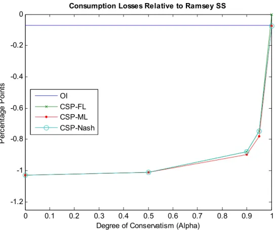
We illustrate this point in figure 1, for the baseline calibration of section 5. The figure displays the steady state welfare gains associated with intermediate degrees of monetary conservatism 5 [0>1], for all the timing arrangements. The upper horizontal line shown in the figure indicates the welfare losses of the OI regime. For the Nash and monetary leadership (ML) regimes, a fully conservative monetary authority (= 1) approximately implements the steady state welfare level associated with the OI regime.18 Thus, even in a situation
with simultaneous decisions or monetary leadership, it remains possible to re-cover the significant welfare losses resulting from lack of monetary commitment 1 8As will become clear from figure 2 below, the welfare level of the OI regime is actually
through an appropriate degree of monetary conservatism. Interestingly, most of the welfare gains are achieved for values ofabove 0.9, i.e., by a su!ciently conservative central bank caring almost exclusively about inflation.
Using again the baseline calibration, figure 2 illustrates how the steady state values of private consumption, labor eort, inflation and public spending de-pend on the degree of monetary conservatism. While an increase in monetary conservatism reduces the inflation bias for all timing protocols, its eect on the fiscal spending bias depends on whether or not fiscal policy takes into account the monetary policy reaction. If fiscal policy takes monetary decisions as given, monetary conservatism results in an increased fiscal spending bias. Nevertheless, the figure shows that an inflation conservative central bank remains desirable in the Nash and ML regimes, as a value ofslightly below one recovers the OI outcome.
6.3
Implications for Stabilization Policy
Up to this point we restricted attention to steady state outcomes. This section extends the analysis to a stochastic economy, considering stabilization policy in response to technology and mark-up shocks. We thereby restrict attention to the sequential policy regime that implements the Ramsey steady state, i.e., fiscal leadership and full monetary conservatism ( = 1).19 We compare the
impulse responses for this policy regime with the Ramsey response to shocks. We start by deriving conditions under which the Ramsey response can be implemented by the sequential policy regime. Clearly, full monetary conser-vatism implies that the central bank will implement stable prices at all times. Therefore, a necessary condition for the optimality of the impulse response un-der the consiun-dered policy arrangement is that the Ramsey allocation can be implemented with a stable price path. The next proposition states that this is also a su!cient condition:
Proposition 10 If the Ramsey response to shocks can be implemented with a stable path for prices, then it is consistent with sequential policymaking in a regime with fiscal leadership and fully conservative monetary policy (= 1).
The proof is given in appendix A.11; it involves showing that the first or-der conditions of the Ramsey problem with stable prices are identical to those implied by fiscal leadership and a fully conservative monetary authority.
Given the result of proposition 10 the next question is then under which conditions the Ramsey policy response may involve a stable price path in re-sponse to shocks. The following proposition provides su!cient conditions for the response to a technology shock.
1 9Since it is not obvious how to compare impulse responses across policy regimes involving
Proposition 11 Assume preferences over fw> kw andjw are of the constant rel-ative risk class. If private and public consumption have the same coe!cient of relative risk aversion and{= 0, then the Ramsey response to a technology shock involves no deviation from price stability.
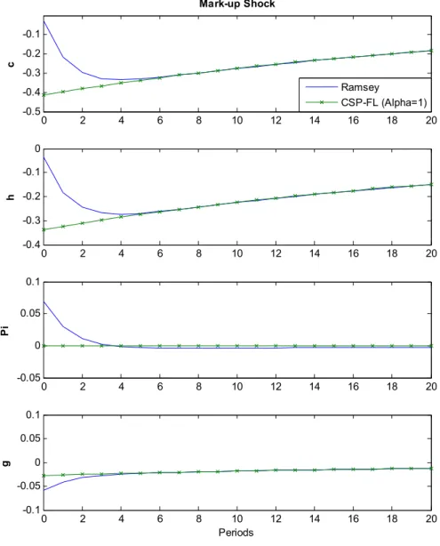
The proof is given in appendix A.12. The proof shows that price stability is optimal if the Ramsey response implies a stable private consumption to output ratio as well as a stable public consumption to output ratio. Maintaining both ratios constant is not possible in the presence of a positive and constant level of fiscal waste ({ A0), because total output responds to technology shocks. Thus, sequential policymaking with fiscal leadership and a fully conservative central bank will generally fail to implement the Ramsey response to a technology shock. We now turn to the case of a mark-up shock. The Ramsey response then generally involves deviations from price stability, even if the assumptions of proposition 11 are satisfied. We illustrate this point in figure 2 for the baseline parametrization of section 5. The figure depicts the impulse responses to a positive mark-up shock under the Ramsey policy, as well as for the case with fiscal leadership and a fully conservative central bank.20 While the Ramsey response involves an initial increase in inflation followed by a small but persistent amount of deflation, the sequential policy regime implements stable prices at all times. Overall, the deviations from price stability under the Ramsey policy seem small (in the order of less than 0.1% per quarter) and the responses dier across regimes only for the early periods following a shock.
The following proposition provides an explanation for why the response un-der sequential policy turns out to be so similar to the Ramsey response. The proof is given in appendix A.13.
Proposition 12 Sequential policymaking in a regime with fiscal leadership and fully conservative monetary policy ( = 1) is consistent with the Ramsey re-sponse to shocks under flexible prices.
A regime with fiscal leadership and full monetary conservatism eliminates all gaps to the Ramsey equilibrium with flexible prices. The presence of sticky prices, however, may allow the Ramsey planner to improve somewhat upon the flexible price response, see Adao et al. (2003). While the stabilization policy associated with fiscal leadership and full monetary conservatism may not be always fully optimal, the previous proposition suggests that such a policy arrangement remains close to fully optimal as it implements the optimal flexible price equilibrium.
2 0Responses are for a positive three standard deviation of the mark-up shock, and presented
7
Conclusions
This paper analyzes the policy biases associated with sequential monetary and fiscal policymaking in a stylized dynamic stochastic general equilibrium model. The paper also asks whether installing an inflation conservative central bank remains desirable in a setting with endogenous fiscal policy.
While the lack of fiscal commitment can make it optimal to implement pos-itive inflation rates (for simultaneous decision making or monetary leadership), the optimal deviations from price stability turn out to be quantitiatively small. In addition, the inflation bias resulting from lack of monetary commitment tends to generate too much inflation for a wide range of model parameterizations. In-stalling a conservative central bank is therefore welfare improving.
In a setting with fiscal leadership, arguably the most relevant case, installing a fully conservative central bank focusing exclusively on stabilizing inflation eliminates not only the inflation bias but also the fiscal spending bias in steady state. The case for monetary conservatism may thus be even stronger in a setting with endogenous fiscal policy. Moreover, fiscal leadership with full conservatism implements the optimal stabilization policy under flexible prices, which tends to be close to optimal if not fully optimal.
A number of important questions remain to be addressed in further research. In particular, for a positive description of monetary and fiscal policy interactions, it seems important to consider also distortionary taxation and government debt dynamics. These elements introduce additional interactions between monetary and fiscal policymakers that may have a major impact on the desirability of an inflation conservative monetary authority. We plan to extend the analysis to such richer settings in future work.
A
Appendix
A.1
Ramsey Steady State
The Lagrangian of the Ramsey problem (12) is
max {fw>kw>w>Uw>jw} H0 4 X w=0 wnx(fw> kw> jw) +w1 xfw(w1)w xfw}wkw μ 1 +w+ xkw xfw w }w ¶ xfw+1(w+11)w+1 ¸ +w2 xfw Uw xfw+1 w+1 ¸ +w3 }wkwfw 2(w1)2jw{ ¸¾
The first-order conditions w.r.t. (fw> kw>w> Uw> jw), respectively, are given by xfw+w1 μ xffw(w1)w xffw}wkw (1 +w) ¶ w1 1xffw(w1)w+w2 xffw Uw w2 1xffw w 3w = 0 (22) xkww1 xfw}w μ 1 +w+xkw xfw w }w +kwxkkw xfw w }w ¶ +w3}w= 0 (23) ¡ w11w1¢xfw(2w1) +w2 1 xfw 2w 3 w(w1) = 0 (24) w2xfw U2w = 0 (25) xjw3w = 0 (26)
where m1 = 0for m = 1>2. We denote the Ramsey steady state by dropping time subscripts. Equation (25),xfwA0andUw1imply
2= 0
Equations (26) delivers
3=xjA0
This and equation (24) gives
= 1
From (9) it then follows
U= 1
Then equation (8) delivers
1 ++xk xf
This delivers (13) shown in the main text. Using the previous results, equation (23) simplifies to
xk1 k
xkk+xj= 0 (28)
From (22) one obtains
1k
=
xfxj xff(1 +)
(29) Substituting (29) into (28) delivers
xk
xfxj xff(1 +)
xkk+xj= 0
Using (27) to substitute forxf one gets
xj=xk 1 +³ 1+ ´2x kk xff 1 + 1+xxkkff
Using (27) again to substitute 1+ delivers (14) shown in the main text.
A.2
Sequential Fiscal Reaction Function
The fiscal problem (15) is
max {fw+m>kw+m>w+m>jw+m} Hw 4 X m=0 mnx(f w+m> kw+m> jw+m) +w1+m xfw+m(w+m1)w+m xfw+m}w+mkw+m μ 1 +w+m+ xkw+m xfw+m w+m }w+m ¶ xfw+m+1(w+m+11)w+m+1 i +w2+m xfw+m Uw+m xfw+m+1 w+m+1 ¸ +3w+m }w+mkw+mfw+m 2(w+m1)2jw+m{ ¸¾
taking as givenUw+m1and other variables datedw+m form1. The first order conditions w.r.t. (fw> kw>w> jw), respectively, are given by
xfw+1w μ xffw(w1)w xffw}wkw (1 +w) ¶ +w2xffw Uw w3= 0 (30) xkw1w xfw}w μ 1 +w+ xkw xfw w }w +kw xkkw xfw w }w ¶ +w3}w= 0 (31) w1xfw(2w1)w3(w1) = 0 (32) xjww3= 0 (33)
From equations (32) and (33) one gets
w1=xjw(w1) xfw(2w1)
Using the previous result and (33) to substitute the Lagrange multipliers in (31) delivers FRF shown in the main text.
A.3
Sequential Monetary Reaction Function
The monetary problem (17) is
max {fw+m>kw+m>w+m>Uw+m} Hw 4 X m=0 mnx(fw+m> kw+m> jw+m) +w1+m xfw+m(w+m1)w+m xfw+m}w+mkw+m μ 1 +w+m+ xkw+m xfw+m w+m }w+m ¶ xfw+m+1(w+m+11)w+m+1 i +w2+m xfw+m Uw+m xfw+m+1 w+m+1 ¸ +3w+m }w+mkw+mfw+m2(w+m1)2jw+m{ ¸¾
taking as givenjw+m1and other variables datedw+m form1. The first order conditions w.r.t. (fw> kw>w> Uw)are given by
xfw+1w μ xffw(w1)w xffw}wkw (1 +w) ¶ +w2xffw Uw w3= 0 (34) xkw1w xfw}w μ 1 +w+xkw xfw w }w +kwxkkw xfw w }w ¶ +w3}w= 0 (35) w1xfw(2w1)w3(w1) = 0 (36) w2xfw U2w = 0 (37)
Equation (37),xfwA0andUw1imply w2= 0
Then solving (34), (35) and (36) forw3 delivers, respectively,
w3=xfw+w1 μ xffw(w1)w xffw}wkw (1 +w) ¶ (38) w3=xkw }w +1wxfw μ 1 +w+ xkw xfw w }w +kw xkkw xfw w }w ¶ (39) w3=w1xfw(2w1) (w1) (40)
Equations (38) and (40) imply w1= 2 w1 w1 xffw xfw ((w1)w}wkw(1 +w)) (41) While equations (39) and (40) give
1w = }wxfw xkw ³ 1 +w2ww11+xxkwfw }ww +kwxxkkwfw }ww ´ (42)
From (41) and (42) one obtains MRF shown in the main text.
A.4
Proof of Proposition 2
We first show that MRF cannot hold in the neighborhood of= 1. In steady state one can rewrite MRF as
μ 1 + xf xk ¶ +R(1) = 0 (43)
whereR(1)summarizes terms that converge to zero as (1) $0. In a steady state with= 1equation (8) delivers 1 ++xk
xf = 0and thus xf xk ?
1+ ?1. Since the implicit function xf
xk()defined by (8) exists, this implies
that xf
xk is bounded away from 1 also in a su!ciently small neighborhood
around = 1. Therefore, (43) cannot hold in the neighborhood of = 1. Moreover, fromU1and (9) we havein steady state. Forsu!ciently close to 1, it then follows that MRF can only hold ifA1.
A.5
Proof of Proposition 4
The eect of inflation on steady state utility is given by
gx g =xf Cf C+xk Ck C+xj Cj C (44)
where f()> k()> j() denote the steady state levels emerging under sequen-tial fiscal policy when monetary policy implements inflation rate , and the derivativesxm (m =f> k> j)are evaluated at this steady state. We first evaluate
equation (44) at= 1. Equation (8) simplifies to
xf=
1 +xk (45)
Totally dierentiating equation (10) and evaluating at= 1 gives
Cf C = Ck C Cj C
Using this result and (16), equation (44) can be rewritten as
gx
g = (xfxj)
Cf C
Equations (16) and (45) implyxfA xj, thus vljq μ gx g ¶ =vljq μ Cf C ¶ (46) To determine the sign of Cf@C we totally dierentiate equations (FRF), (8), (10) and evaluate at= 1, this delivers
3 C 0 xkk xjj k xkxx2ff f k xxkkf 0 1 1 1 4 D 3 C Cf C Ck C Cj C 4 D= 3 C kxkxkk xf 0 0 4 D
Solving for CCf and CCj gives
Cf C = xfxkk xfxkkxjjxffxkxjjxffxkxkk kxkxkk xf Cj C = xfxkk+xffxk xfxkkxjjxffxkxjjxffxkxkk kxkxkk xf
Assumingxkk ?0, signing these expression delivers CCf A 0 and CCj ? 0, as
claimed. The former inequality and equation (46) imply ggx A 0, locally at
= 1.
A.6
Utility Weights
For the period utility specification (18), the Ramsey policy marginal conditions (13) and (14), respectively, deliver
$k= 1 fk* 1 + (47) $j=$kjk* 1 + 1+kf* 1 + f k* (48) Assuming f = 0=16, k = 0=2, j = 0=04, = 6 and * = 1 one obtains the parameter values in table 1.
A.7
Solving for the Equilibrium with Sequential
Mone-tary and Fiscal Policy
The Markov-perfect Nash equilibrium with sequential monetary and fiscal policy solves the following problem
max {fw+m>kw+m>w+m>Uw+m>jw+m} Hw 4 X m=0 mx(fw+m> kw+m> jw+m) (49) s.t.
Equations (8),(9),(10) for allw
Hw(fw+m> kw+m>w+m> Uw+m> jw+m) given form1
One should note that FRF and MRF need not be imposed, since they can already be derived from the first order conditions of this problem, see sections 4.3.1 and 4.3.2, respectively. Therefore, the solution of problem (49) will always satisfy FRF and MRF.
Then, the recursive formulation of the Lagrangian of problem (49) is
Z(}w> w) = min (w1>2w>w3) max (fw>kw>w>Uw>jw){ i(·) +HwZ(}w+1> w+1)} (50) s.t. }w+1= (1}) +}}w+%}w+1 w+1=(1) +w+%w+1 where the one-period return is
i(·) =x(fw> kw> jw) +w1 xfw(w1)wxfw}wkw μ 1 +w+xkw xfw w }w ¶ HDVw ¸ +w2 xfw Uw H LV w ¸ +w3 }wkwfw 2(w1)2jw{ ¸
with the expectations functions
HDV
w Hwxfw+1(w+11)w+1 (51)
HwLV Hw xfw+1
w+1 (52)
taken as given. The additional control variablesw1, w2, w3 are the Lagrange multipliers associated with the implementability constraints (8) and (9), and the feasibility constraint (10), respectively.
We then solve for the steady state using the first order conditions of the recursive formulation (50). Thereafter, we compute a quadratic approximation
of the one-period returni(·) around this steady state. This involves quadrat-ically approximating the implementability and feasibility constraints. Instead, the expectation functionsHDV
w andHwLV are linearly approximated as
HwDV d10+d11(}w1) +d12(w) (53) HwLV d20+d21(}w1) +d22(w) (54)
Importantly, postulating linear expectation functions is su!cient to obtain a first order approximation to the equilibrium dynamics and policy functions. The policymaker takes expectations functions as given, therefore, they do not show up in dierentiated form in the first order conditions. Moreover, linear expectations functions are su!cient to evaluate the Lagrangian, i.e., utility, up to second order. This is the case since either the implementability constraints or the associated Lagrange multipliers are zero in a su!ciently small neighborhood around the steady state. As a result, no first order terms appear when evaluating the quadratic approximation ofi(·) at the solution. Obviously, this is just a restatement of the fact that (50) is an unconstrained optimization problem.
We now explain how we compute the expectation functions (53) and (54). We start with an initial guess for dml (m = 1>2; l = 0>1>2), then we solve (50) withi(·)replaced by its quadratic approximation. We updateml, as explained below, and continue iterating until the maximum absolute change of the policy functions drops below the square root of machine precision, i.e.,1=49·108.
Let the solution for the policy functionsf(·)and(·)be given by
fw+1f=f}(}w+11) +f(w+1) (55)
w+1=}(}w+11) +(w+1) (56)
where variables without time subscript denote steady state values. A first order approximation of the expectation functions (51) and (52) then delivers
HwDV HDVw ¯¯vv+ CH DV w Cfw+1 ¯¯ ¯¯ vv Hw(fw+1f) + CH DV w Cw+1 ¯¯ ¯¯ vv Hw(w+1) HwLV HLVw ¯¯vv+ CH LV w Cfw+1 ¯¯ ¯¯ vv Hw(fw+1f) + CH LV w Cw+1 ¯¯ ¯¯ vv Hw(w+1)
where|vv indicates expressions evaluated at steady state. These together with
(55), (56) and
Hw(}w+11) =}(}w1) Hw(w+1) =(w)
deliver the expectations functions consistent with the approximated policy func-tions
d10=xf(1) d11=}[(1)xfff}+xf(21)}] d12=[(1)xfff+xf(21)] d20=xf d21=} £ xfff}xf} ¤ d22= £ xfffxf ¤
A.8
Consumption Losses Relative to Ramsey
Let x(f> k> j) denote the period utility for the Ramsey steady state and let
x¡fD> kD> jD¢represent the period utility for the steady state of an alternative
policy regime. The permanent reduction in private consumption that would imply the Ramsey steady state to be welfare equivalent to the alternative policy regimeD0is implicitly defined by
1 1x ¡ fD> kD> jD¢=1 1 x ¡ f(1 +D)> k> j¢ = 1 1 £ x(f> k> j) + log¡1 +D¢¤
where the second equality uses equation (18). Therefore, one obtains
D= exp£x¡fD> kD> jD¢x(f> k> j)¤1
A.9
Conservative Monetary Reaction Function
The conservative monetary problem (19) is
max {fw+m>kw+m>w+m>Uw+m} Hw 4 X m=0 mn(1)x(fw+m> kw+m> jw+m)2(w1)2 +w1+m xfw+m(w+m1)w+m xfw+m}w+mkw+m μ 1 +w+m+ xkw+m xfw+m w+m }w+m ¶ xfw+m+1(w+m+11)w+m+1 i +w2+m xfw+m Uw+m xfw+m+1 w+m+1 ¸ +3w+m }w+mkw+mfw+m 2(w+m1)2jw+m{ ¸¾
taking as given jw+m1 and variables dated w+m for m 1. The first order conditions w.r.t. (fw> kw>w> Uw), respectively, are given by
(1)xfw+w1 μ xffw(w1)wxffw}wkw (1 +w) ¶ +w2xffw Uw 3 w = 0 (57) (1)xkww1 xfw}w μ 1 +w+ xkw xfw w }w +kw xkkw xfw w }w ¶ +3w}w= 0 (58) w1xfw(2w1)w3(w1)(w1) = 0 (59) w2xfw U2w = 0 (60)
Equation (60),xfwA0andUw1imply w2= 0
Then solving (57), (58) and (59) forw3 delivers, respectively,
w3= (1)xfw+w1 μ xffw(w1)wxffw}wkw (1 +w) ¶ (61) w3=(1)xkw }w +w1xfw μ 1 +w+ xkw xfw w }w +kw xkkw xfw w }w ¶ (62) w3=1wxfw(2w1) (w1) (63)
Equations (61) and (63) imply
w1= ³1+x1 fw ´ 2w1 w1 xffw xfw ((w1)w}wkw(1 +w)) (64) While equations (62) and (63) give
1w = ³1 }w xkw ´ }wxfw xkw ³ 1 +w2ww11+xxkwfw }ww +kwxxkkwfw }ww ´ (65)
From (64) and (65) one obtains CMRF shown in the main text.
A.10
Proof of Proposition 8
Full monetary conservatism implies that w 1, see CMRF. Substituting w1for (CMRF), noting that (9) can be dropped as it only definesUw, and
using (10) to substitutekw, one can rewrite problem (21) as max {fw+m>jw+m} Hw 4 X m=0 mx(fw+m>fw+m +jw+m+{ }w+m > jw+m) s.t. xk ³ fw+jw+{ }w ´ xf(fw) =}w 1 +w w for allw (66) {fw+m> kw+m> jw+m} given form1
Lettingw denote the Lagrange multiplier on (66), the FOCs w.r.t. (fw> jw> w),
respectively, are given by
xfw+ xkw }w +w xkkw }w xfwxkwxffw (xfw)2 = 0 xkw }w +xjw+w xkkw }w xfw = 0 }w 1 +w w +xkw xfw = 0
Eliminatingwfrom the first FOCs delivers xfw+ xkw }w μ xkw }w +xjw ¶ μ 1}w xkw xkkw xffw xfw ¶ = 0
Using the last FOC above to substitute the term xfw on the left-hand side of
the previous equation gives
xjw= xkw }w 1 w 1+w xkkwxfw }wxkwxffw 1 xkkwxfw }wxkwxffw (67) The sequential equilibrium under fiscal leadership and full monetary conser-vatism is thus described by the solution to (66), (67), (10), w = 1, and (9).
Steady state versions of these equations characterize the Ramsey steady state, see section 4.2.
A.11
Proof of Proposition 10
Appendix A.10 has shown that the equilibrium with fiscal leadership and full monetary conservatism is described by (66), (67), (9), (10), andw1. We now
show that the same equations characterize the Ramsey equilibrium, provided
w1is optimal. Equations (9), (10) and (66) are also constraints imposed on
the Ramsey problem forw1. It thus remains to be shown that the Ramsey
problem also implies (67). Forw1the FOCs of the Ramsey problem
xfw+w1 μ xffw}wkw (1 +w) ¶ xjw= 0 (68) xkw1w xfw}w μ kw xkkw xfw w }w ¶ +xjw}w= 0 (69)
where we used also (66). From (68) we get
w1kw
=
xfwxjw xffw}w(1 +w)
Using this to eliminate1w in (69) and employing again (66) delivers (67).
A.12
Proof of Proposition 11
The FOCs of the Ramsey problem consist of equations (22)-(26), (8), (9), and (10). Using w2 = 0 and w3 = xjw, noting that the Euler equation can be
dropped as it only defines Uw, and setting w = (we are interested in the
impulse response to a technology shock) reduces the FOCs to the following:
xfw+ ¡ w1w1 1¢xffw(w1)ww1 xffw}wkw (1 +)xjw= 0 (70) xkww1 xfw}w μ 1 ++xkw xfw }w +kw xkkw xfw }w ¶ +xjw}w= 0 (71) ¡ w1w1 1¢xfw(2w1)xjw(w1) = 0 (72) xfw(w1)w xfw}wkw μ 1 ++xkw xfw }w ¶ xfw+1(w+11)w+1= 0 (73) }wkwfw2(w1)2jw{= 0 (74)
We now show that these FOCs are satisfied for a stable price path under the assumptions stated in the proposition. (73) holds forw= 1if
xkw xfw 1 }w = xk xf =1 + (75)
where expressions without time subscript denote steady state values. From (72) follows thatw= 1 also requires
w1=1 (76)
Equation (71) and the previous two results then deliver
11