NEHRP Seismic Design Technical Brief No. 4
Nonlinear Structural Analysis
For Seismic Design
A Guide for Practicing Engineers
NIST GCR 10-917-5
Gregory G. Deierlein
Andrei M. Reinhorn
Michael R. Willford
About The Authors
Gregory G. Deierlein, Ph.D., P.E., is a faculty member at Stanford University where he specializes in the design and behavior of steel and concrete structures, nonlinear structural analysis, and performance-based design of structures for earthquakes and other extreme loads. Deierlein is the Director of the John A. Blume Earthquake Engineering Center at Stanford. He is active in national technical committees involved with developing building codes and standards, including those of the American Institute of Steel Construction, the Applied Technology Council, and the American Society of Civil Engineers.
About the Review Panel
The contributions of the three review panelists for this publication are gratefully acknowledged.
Graham H. Powell, Ph.D., is Emeritus Professor of Structural Engineering, University of California at Berkeley and was a lecturer in Civil Engineering, University of Cantebury, New Zealand, 1961-1965. He is a consultant to Computers and Structures Inc., publisher of his text Modeling for Structural Analysis. He has special expertise in seismic resistant design and the modeling of structures for nonlinear analysis. Finley A. Charney, Ph.D., P.E., is an Associate Professor in the Department of Civil and Environmental Engineering at Virginia Polytechnic Institute, Blacksburg, Virginia, and is President of Advanced Structural Concepts, Inc., also located in Blacksburg. Prior to joining Virginia Tech in 2001, Charney accumulated twenty years of experience as a practicing structural engineer. He is the author of many publications on the application of structural analysis methods in seismic design. Mason Walters, S.E., is a practicing structural engineer and a principal with Forell/Elsesser Engineers, Inc. in San Francisco. Walters has been in private practice for over 30 years, focusing on the application of the seismic protective systems for numerous significant buildings and bridge projects. Examples of these projects include the elevated BART/Airport Light Rail Station at San Francisco International Airport, and the seismic isolation retrofit of the historic Oakland City Hall. Many of Mr. Walters’ projects have incorporated nonlinear dynamic and static analysis procedures.
National Institute of
Standards and Technology
The National Institute of Standards and Technology (NIST) is a federal technology agency within the U.S. Department of Commerce that promotes U.S. innovation and industrial competitiveness by advancing measurement science, standards, and technology in ways that enhance economic security and improve our quality of life. It is the lead agency of the National Earthquake Hazards Reduction Program (NEHRP). Dr. John (Jack) R. Hayes is the Director of NEHRP, within NIST’s Building and Fire Research Laboratory (BFRL). Dr. Kevin K. F. Wong managed the project to produce this Technical Brief for BFRL.NEHRP Consultants Joint Venture
This NIST-funded publication is one of the products of the work of the NEHRP Consultants Joint Venture carried out under Contract SB 134107CQ0019, Task Order 69195. The partners in the NEHRP Consultants Joint Venture are the Applied Technology Council (ATC) and the Consortium of Universities for Research in Earthquake Engineering (CUREE). The members of the Joint Venture Management Committee are James R. Harris, Robert Reitherman, Christopher Rojahn, and Andrew Whittaker, and the Program Manager is Jon A. Heintz. Assisting the Program Manager is ATC Senior Management Consultant David A. Hutchinson, who on this Technical Brief provided substantial technical assistance in the development of the content.
Consortium of Universities for Research in Earthquake Engineering (CUREE) 1301 South 46th Street - Building 420 Applied Technology Council (ATC)
201 Redwood Shores Parkway - Suite 240 Redwood City, California 94065
NEHRP Seismic Design
Technical Briefs
NEHRP (National Earthquake Hazards Reduction Program) Technical Briefs are published by NIST, the National Institute of Standards and Technology, as aids to the efficient transfer of NEHRP and other research into practice, thereby helping to reduce the nation’s losses from earthquakes.
Andrei Reinhorn, Ph.D., S.E., is a professor at the University at Buffalo. He has published two books and authored two computer platforms (IDARC and 3D-BASIS) for nonlinear analysis of structures and for base isolation systems. He has served as Director of the Structural Engineering and Earthquake Engineering Laboratory at the University at Buffalo.
Michael R. Willford, M.A., C.Eng. is a Principal of the global consulting firm Arup with 35 years experience of design of structures for buildings, civil, and offshore projects in many parts of the world. A specialist in structural dynamics, he is leader of Arup’s Advanced Technology and Research practice, specializing in the development and application of innovative design techniques using performance-based methods.
By Gregory G. Deierlein, Ph.D., P.E. Stanford University Stanford, California Andrei M. Reinhorn, Ph.D., S.E. University at Buffalo, SUNY Buffalo, New York Michael R. Willford, M.A., C.Eng. Arup San Francisco, California
October 2010 Prepared for
U.S. Department of Commerce Building and Fire Research Laboratory National Institute of Standards and Technology Gaithersburg, MD 20899-8600
Nonlinear Structural Analysis
For Seismic Design
A Guide for Practicing Engineers
NIST GCR 10-917-5
U.S. Department of Commerce
Gary Locke, Secretary
National Institute of Standards and Technology
Disclaimers
The policy of the National Institute of Standards and Technology is to use the International System of Units (metric units) in all of its publications. However, in North America in the construction and building materials industry, certain non-SI units are so widely used instead of SI units that it is more practical and less confusing to include measurement values for customary units only in this publication. This publication was produced as part of contract SB134107CQ0019, Task Order 69195 with the National Institute of Standards and Technology. The contents of this publication do not necessarily reflect the views or policies of the National Institute of Standards and Technology or the US Government.
This Technical Brief was produced under contract to NIST by the NEHRP Consultants Joint Venture, a joint venture of the Applied Technology Council (ATC) and the Consortium of Universities for Research in Earthquake Engineering (CUREE). While endeavoring to provide practical and accurate information in this publication, the NEHRP Consultants Joint Venture, the authors, and the reviewers do not assume liability for, nor make any expressed or implied warranty with regard to, the use of its information. Users of the information in this publication assume all liability arising from such use.
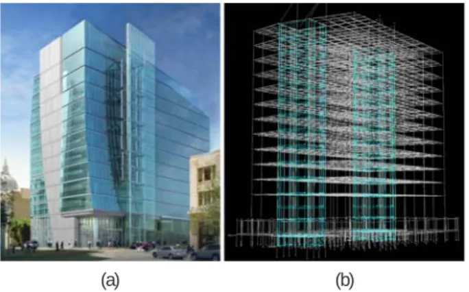
Cover photo – Nonlinear analysis model for a seismic retrofit study of an existing building with concrete shear walls.
How to Cite This Publication
Deierlein, Gregory G., Reinhorn, Andrei M., and Willford, Michael R. (2010). “Nonlinear structural analysis for seismic design,” NEHRP Seismic Design Technical Brief No. 4, produced by the NEHRP Consultants Joint Venture, a partnership of the Applied Technology Council and the Consortium of Universities for Research in Earthquake Engineering, for the National Institute of Standards and Technology,
Introduction...1
Nonlinear Demand Parameters and Model Attributes...4
Modeling of Structural Components...12
Foundations and Soil Structure Interaction...19
Requirements for Nonlinear Static Analysis...21
Requirements for Nonlinear Dynamic Analysis...23
References...27
Notations and Abbreviations...30
Credits...32
1.
2.
3.
4.
5.
6.
7.
8.
9.
Contents
1.1 The Role and Use of Nonlinear
Analysis in Seismic Design
While buildings are usually designed for seismic resistance using elastic analysis, most will experience significant inelastic deformations under large earthquakes. Modern performance-based design methods require ways to determine the realistic behavior of structures under such conditions. Enabled by advancements in computing technologies and available test data, nonlinear analyses provide the means for calculating structural response beyond the elastic range, including strength and stiffness deterioration associated with inelastic material behavior and large displacements. As such, nonlinear analysis can play an important role in the design of new and existing buildings.
Nonlinear analyses involve significantly more effort to perform and should be approached with specific objectives in mind. Typical instances where nonlinear analysis is applied in structural earthquake engineering practice are to: (1) assess and design seismic retrofit solutions for existing buildings; (2) design new buildings that employ structural materials, systems, or other features that do not conform to current building code requirements; (3) assess the performance of buildings for specific owner/stakeholder requirements (Figure 1-1). If the intent of using a nonlinear analysis is to justify a design that would not satisfy the prescriptive building code requirements, it is essential to develop the basis for acceptance with the building code authority at the outset of a project. The design basis should be clearly defined and agreed upon, outlining in specific terms all significant performance levels (Sidebar 1)
and how they will be evaluated.
1. Introduction
Sidebars in the guide
Sidebars are used in this Guide to illustrate key points, and to provide additional guidance on good practices and open issues in analysis, design, and construction.
Sidebar 1
Performance Levels and Acceptance Criteria The earthquake performance of buildings generally relates to damage incurred to the building’s structure, envelope, partitions, ceilings, mechanical/electrical systems, and contents. While the building performance is a continuum, for design purposes it is convenient to identify discrete performance levels for the major
structural and other building components that significantly
affect building function, property protection, and safety. ASCE 41 (ASCE 2007) and other standards generally provide guidance on three performance levels:
Immediate Occupancy – Achieve essentially elastic behavior by limiting structural damage (e.g., yielding of steel, significant cracking of concrete, and nonstructural damage.)
Life Safety - Limit damage of structural and nonstructural components so as to minimize the risk of injury or casualties and to keep essential circulation routes accessible.
Collapse Prevention – Ensure a small risk of partial or complete building collapse by limiting structural
deformations and forces to the onset of significant
strength and stiffness degradation.
ASCE 41 provides acceptance criteria in terms of deformation and force demands on individual structural components. Other demand parameters (especially
story drifts and floor accelerations) are also important
indicators of damage to nonstructural components and overall building performance (PEER 2010; Willford et al. 2008; PEER/ATC 2010; ATC 2009). Moreover, there
may be other significant performance limits (such as
onset of damage to the building envelope) that have major implications on lifecycle cost and functionality. While the risk (or likelihood) of exceeding the damage
specified in performance levels is predicated by building
occupancy and other factors, for typical buildings, i.e., Occupancy Category II in ASCE 7 (ASCE 2010), it is generally accepted to check the Collapse Prevention performance level for the Maximum Considered Earthquake ground motion intensity and Life Safety
for the Design Basis Earthquake (defined as 2/3 of the
Maximum Considered Earthquake intensity in ASCE 7). The appropriate ground motion intensity for checking
Immediate Occupancy is less well-defined, since this
performance level is not typically addressed in building codes.
•
•
•
Figure 1-1 – New headquarters of San Francisco Public Utility Commission Building designed using nonlinear response history analysis
to meet stringent immediate occupancy performance criteria. (b)
Once the goals of the nonlinear analysis and design basis are defined, the next step is to identify specific demand parameters and appropriate acceptance criteria to quantitatively evaluate the performance levels. The demand parameters typically include peak forces and deformations in structural and nonstructural components, story drifts, and floor accelerations. Other demand parameters, such as cumulative deformations or dissipated energy, may be checked to help confirm the accuracy of the analysis and/or to assess cumulative damage effects.
In contrast to linear elastic analysis and design methods that are well established, nonlinear inelastic analysis techniques and their application to design are still evolving and may require engineers to develop new skills. Nonlinear analyses require thinking about inelastic behavior and limit states that depend on
Sidebar 2
Capacity Design
Capacity design is an approach whereby the designer establishes which elements will yield (and need to be ductile) and those which will not yield (and will be
designed with sufficient strength) based on the forces
imposed by yielding elements. The advantages of this strategy include:
Protection from sudden failures in elements that cannot be proportioned or detailed for ductile response.
Limiting the locations in the structure where expensive ductile detailing is required.
Greater certainty in how the building will perform
under strong earthquakes and greater confidence in
how the performance can be calculated.
Reliable energy dissipation by enforcing deformation modes (plastic mechanisms) where inelastic deformations are distributed to ductile components. The well known “strong column/weak beam” requirement is an example of a capacity design strategy, where the intent is to avoid inelastic hinging in columns that could lead to premature story mechanisms and rapid strength degradation in columns with high axial loads. The design of yielding links and elastic braces in eccentrically braced frames is another example of capacity design. Where inelastic analysis is used, capacity design can be
implemented by modeling the specified yielding elements
with their “expected” strengths and the protected elements as elastic. This permits the determination of and design for the maximum expected force demands in the protected elements.
deformations as well as forces. They also require definition of component models that capture the force-deformation response of components and systems based on expected strength and stiffness properties and large deformations. Depending on the structural configuration, the results of nonlinear analyses can be sensitive to assumed input parameters and the types of models used. It is advisable to have clear expectations about those portions of the structure that are expected to undergo inelastic deformations and to use the analyses to (1) confirm the locations of inelastic deformations and (2) characterize the deformation demands of yielding elements and force demands in non-yielding elements. In this regard, capacity design concepts are encouraged to help ensure reliable performance (Sidebar 2).
While nonlinear analyses can, in concept, be used to trace structural behavior up to the onset of collapse, this requires sophisticated models that are validated against physical tests to capture the highly nonlinear response approaching collapse. Since the uncertainties in calculating the demand parameters increase as the structure becomes more nonlinear, for design purposes, the acceptance criteria should limit deformations to regions of predictable behavior where sudden strength and stiffness degradation does not occur.
This Technical Brief is intended to provide a summary of the important considerations to be addressed, considering the current capabilities of nonlinear analysis technologies and how they are being applied in practice. The scope includes both nonlinear static (pushover) and dynamic (response history) analyses, but with the emphasis towards the latter. This guide is intended to be consistent with building codes and standards, however, as the use of nonlinear analysis for design is still evolving, there are many areas where details of the implementation are open to judgment and alternative interpretations. Finally, while this technical brief is concerned primarily with buildings, the guidance can generally apply to nonlinear analysis of other types of structures.
1.2 Background on Use of Nonlinear
Analysis in Building Design in the USA
The first widespread practical applications of nonlinear analysis in earthquake engineering in the USA were to assess and retrofit existing buildings. The first significant guidelines on the application of nonlinear analysis were those published in FEMA 273 NEHRP Guidelines for the Seismic Rehabilitation of Buildings (FEMA 1997) and ATC 40 Seismic Evaluationand Retrofit of Concrete Buildings (ATC 1996). Owing to the state of knowledge and computing technologies at the time of their publication (mid-1990s), these documents focus primarily on nonlinear static (pushover) analysis. They have since been carried forward into ASCE 41 Seismic Rehabilitation of Existing Buildings (ASCE 2007), and improvements have been proposed in FEMA 440 Improvement of Nonlinear Static Seismic Analysis Procedures (FEMA 2005) and FEMA P440A Effects of Strength and Stiffness Degradation on Seismic Response (FEMA
•
• •
2009a). Note that while ASCE 41 and related documents have a primary focus on renovating existing buildings, the nonlinear analysis guidance and component modeling and acceptance criteria in these documents can be applied to new building design, provided that the chosen acceptance criteria provide performance levels expected for new building design in ASCE 7 (Sidebar 1).
About the same time that FEMA 273 and ATC 40 were under development, nonlinear analysis concepts were also being introduced into methods for seismic risk assessment, the most widely known being HAZUS (Kircher et al. 1997a; Kircher et al. 1997b; FEMA 2006). In particular, the building-specific loss assessment module of HAZUS employs nonlinear static analysis methods to develop earthquake damage fragility functions for buildings in the Earthquake Loss Estimation Methodology, HAZUS99-SR2, Advanced Engineering Building Module (FEMA 2002).
More recently, the role of nonlinear dynamic analysis for design is being expanded to quantify building performance more completely. The ATC 58 Guidelines for Seismic Performance Assessment of Buildings (ATC 2009) employ nonlinear dynamic analyses for seismic performance assessment of new and existing buildings, including fragility models that relate structural demand parameters to explicit damage and loss metrics. Nonlinear dynamic analyses are also being used to assess the performance of structural systems that do not conform to prescriptive seismic force-resisting system types in ASCE 7 Minimum Design Loads for Buildings and Other Structures
(ASCE 2010). A significant impetus for this is in the design of tall buildings in high seismic regions, such as outlined in the following documents: Seismic Design Guidelines for Tall Buildings (PEER 2010), Recommendations for the Seismic Design of High-rise Buildings (Willford et al. 2008), and the PEER/ATC 72-1 Modeling and Acceptance Criteria for Seismic
Design and Analysis of Tall Buildings (PEER/ATC 2010).
1.3 Definitions of Terms in this Guide
While structural engineers familiar with the concept of nonlinear analysis for seismic design have been exposed to the following terms in a number of publications, the meanings of these terms have sometimes varied. The following definitions are used in this Guide.
Backbone Curve: Relationship between the generalized force and deformation (or generalized stress and strain) of a structural component or assembly that is used to characterize response in a nonlinear analysis model.
Cyclic Strength Degradation: Reduction in strength, measured
at a given displacement loading cycles, due to reduction in yield strength and stiffness that occurs during the cyclic loading.
Cyclic Envelope: Curve of generalized force versus
deformation that envelopes response data obtained from cyclic loading of a structural component or assembly.
In-Cycle Degradation: Reduction in strength that is associated with negative slop of load versus deflection plot within the same cycle in which yielding occurs.
Monotonic Curve: Curve of generalized force versus
deformation data obtained from monotonic loading of a structural component or assembly.
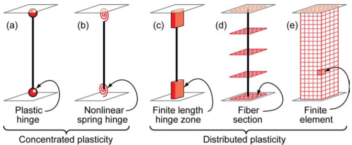
Figure 2-1 – Idealized models of beam-column elements.
2.1 Demand Parameters
Modern performance-based seismic design entails setting performance levels and checking acceptance criteria for which a building is to be designed. Performance levels under defined intensities of ground shaking should be checked using appropriate demand parameters and acceptance criteria. The performance acceptance criteria may be specified for the overall systems, substructures, or components of a building. For a given building and set of demand parameters, the structure must be modeled and analyzed so that the values of the demand parameters are calculated with sufficient accuracy for design purposes. The performance is checked by comparing the calculated values of demand parameters (in short the “demands”) to the acceptance criteria (“capacities”) for the desired performance level. The calculated demands and acceptance criteria are often compared through “demand-capacity” ratios. The acceptance criteria for seismic performance may vary depending on whether static or dynamic nonlinear analysis is used and how uncertainties associated with the demands and acceptance criteria are handled. For example, the component models, demand parameters, and acceptance criteria used in nonlinear static procedures need to implicitly account for cyclic degradation effects that are not modeled in the static analysis. On the other hand, some dynamic analysis models may directly incorporate degradation due to cyclic loading, in which case different models and acceptance criteria may be used. Acceptance criteria for structural components generally distinguished between “deformation-controlled” (ductile components that can tolerate inelastic deformations) and “force-controlled” (non-ductile components whose capacities are governed by strength). In reality, most components exhibit some amount of inelastic deformation, and the distinction between force- and deformation-controlled components
2. Nonlinear Demand Parameters and Model Attributes
is not absolute. Nevertheless, the distinction provides a practical approach to establish requirements for the analysis and design. Deformation-controlled components must be modeled as inelastic, whereas force-controlled components may be modeled as elastic, provided that the force demands do not imply significant yielding in the components. ASCE 41 defines deformation and strength acceptance criteria for Immediate Occupancy, Life Safety, and Collapse Prevention performance levels, and PEER/ATC 72-1 provides guidance on criteria for the onset of structural damage and significant strength/stiffness degradation.
Displacements, velocities, and accelerations are additional demand parameters that can provide insights into the overall building response and damage to nonstructural components and contents. Story racking deformations (which can often be approximated as story drift ratios) provide a good measure of overall structural response, including the vertical distribution of deformations and global torsion of the building, and demands in deformation-sensitive components, such as the building façade, interior partitions, or flexible piping systems. Peak floor accelerations and velocities are commonly used to design and assess performance of stiff acceleration-sensitive building components, such as rigidly anchored equipment, raised floor systems, braced ceiling systems, and rigid piping systems.
2.2 Structural Analysis Model Types
Inelastic structural component models can be differentiated by the way that plasticity is distributed through the member cross sections and along its length. For example, shown in
Figure 2-1 is a comparison of five idealized model types for
simulating the inelastic response of beam-columns. Several types of structural members (e.g., beams, columns, braces, and some flexural walls) can be modeled using the concepts illustrated in Figure 2-1:
The simplest models concentrate the inelastic deformations at the end of the element, such as through a rigid-plastic hinge (Figure 2-1a) or an inelastic spring with hysteretic
properties (Figure 2-1b). By concentrating the plasticity in zero-length hinges with moment-rotation model parameters, these elements have relatively condensed numerically efficient formulations.
The finite length hinge model (Figure 2-1c) is an efficient
distributed plasticity formulation with designated hinge zones at the member ends. Cross sections in the inelastic hinge zones are characterized through either nonlinear moment-curvature relationships or explicit fiber-section integrations that enforce the assumption that plane sections remain plane. The inelastic hinge length may be fixed or variable, as determined from the moment-curvature characteristics of the section together with the concurrent moment gradient and axial force. Integration of deformations along the hinge length captures the spread of yielding more realistically than the concentrated hinges, while the finite hinge length facilitates calculation of hinge rotations.
The fiber formulation (Figure 2-1d) models distribute
plasticity by numerical integrations through the member cross sections and along the member length. Uniaxial material models are defined to capture the nonlinear hysteretic axial stress-strain characteristics in the cross sections. The plane-sections-remain-plane assumption is enforced, where uniaxial material “fibers” are numerically integrated over the cross section to obtain stress resultants (axial force and moments) and incremental moment-curvature and axial force-strain relations. The cross section parameters are then integrated numerically at discrete sections along the member length, using displacement or force interpolation functions (Kunnath et al. 1990, Spacone et al. 1996). Distributed fiber formulations do not generally report plastic hinge rotations, but instead report strains in the steel and concrete cross section fibers. The calculated strain demands can be quite sensitive to the moment gradient, element length, integration method, and strain hardening parameters on the calculated strain demands. Therefore, the strain demands and acceptance criteria should be benchmarked against concentrated hinge models, for which rotation acceptance criteria are more widely reported. The most complex models (Figure 2-1e) discretize the
continuum along the member length and through the cross sections into small (micro) finite elements with nonlinear hysteretic constitutive properties that have numerous input parameters. This fundamental level of modeling offers the most versatility, but it also presents the most challenge in terms of model parameter calibration and computational resources. As with the fiber formulation, the strains calculated from the finite elements can be difficult to
Sidebar 3:
Distributed Versus Concentrated Plasticity Elements
While distributed plasticity formulations (Figures 2-1c to 2-1e) model variations of the stress and strain through the section and along the member in more detail, important local behaviors, such as strength degradation
due to local buckling of steel reinforcing bars or flanges, or the nonlinear interaction of flexural and shear, are difficult to capture without sophisticated and numerically
intensive models. On the other hand, phenomenological concentrated hinge/spring models (Figure 2-1a and 2-1b), may be better suited to capturing the nonlinear degrading response of members through calibration using member test data on phenomenological moment-rotations and hysteresis curves. Thus, when selecting analysis model types, it is important to understand (1)
the expected behavior, (2) the assumptions, and (3) the
approximations inherent to the proposed model type. While more sophisticated formulations may seem to offer better capabilities for modeling certain aspects of
behavior, simplified models may capture more effectively
the relevant feature with the same or lower approximation.
It is best to gain knowledge and confidence in specific
models and software implementations by analyzing
small test examples, where one can interrogate specific
behavioral effects.
interpret relative to acceptance criteria that are typically reported in terms of hinge rotations and deformations. Concentrated and finite length hinge models (Figures 2-1a
through Figure 2-1c) may consider the axial force-moment
(P-M) interactions through yield surfaces (see Figure 2-2). On the other hand, fiber (Figure 2-1d) and finite element (Figure 2-1e) models capture the P-M response directly. Note that while the detailed fiber and finite element models can simulate certain behavior more fundamentally, they are not necessarily capable of modeling other effects, such as degradation due to reinforcing bar buckling and fracture that can be captured by simpler phenomenological models (Sidebar 3).
Some types of concentrated hinge models employ axial load-moment (P-M) yield surfaces. Whereas these models generally do a good job at tracking the initiation of yielding under axial load and bending, they may not capture accurately the post-yield and degrading response. On the other hand, some hinge elements with detailed moment-rotation hysteresis models (Figure 2-3) may not capture P-M interaction, except to the extent that the moment-rotation response is defined based on average values of axial load and shear that are assumed to be present in the hinge. A simple check on the model capabilities •
•
•
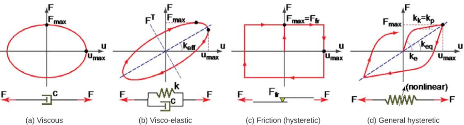
Figure 2-3 – Types of hysteretic modeling.
Figure 2-2 – Idealized axial-force-moment demands and strength interaction surfaces.
(a) Steel columns (b) Concrete walls and columns
(a) Hysteretic model
without deterioration (b) Model with stiffness degradation strength degradation(c) Model with cyclic
(d) Model with fracture
is to analyze a concrete column under a low and high value of axial load (above and below the compression failure balance point) to examine whether the model tracks how the axial load affects the differences in rotation capacity and post-peak degradation. A further check would be to vary the axial loading during the analysis to see how well the effect of the changing axial load is captured.
Sidebar 4
Monotonic Versus Cyclic Envelope Curve
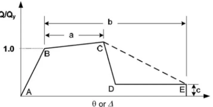
ASCE 41 and other documents provide standardized backbone relationships (Figure 2-7) between characteristic
forces and deformations of structural components to define component behavior, demand parameters, and
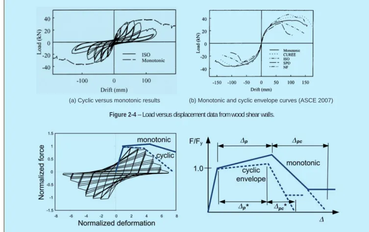
acceptance criteria. For use in nonlinear analysis, it is important to distinguish between so-called “monotonic” and “cyclic envelope” curves. The monotonic curve represents the response that would be observed for a component tested under monotonic loading, and the cyclic envelope encloses the forces and displacements under cyclic loading. As shown below (Figures 2-4 and 2-5), the cyclic envelope varies depending on the applied cyclic loading history, and backbone curves derived from cyclic envelopes are typically based on standardized loading protocols. For nonlinear static analysis, where the cyclic effects of earthquake loading are not modeled directly
in the analysis, the nonlinear component models should be defined based on the degraded cyclic envelope. For
nonlinear dynamic analysis, the choice of component curves depends on how cyclic degradation is modeled. Direct modeling of cyclic degradation begins with a monotonic backbone curve and degrades this relationship as the analysis proceeds (Ibarra et al. 2005). Indirect modeling does not degrade the component backbone curve.
Instead, it uses the cyclic envelope (with an implied amount of cyclic degradation) to define the component backbone
curve in analysis. Whichever technique is used (direct or indirect), the nonlinear analysis should be exercised under cyclic loading to ensure that the model can represent the degradation observed in tests and implied by model parameters in ASCE 41 or other sources.
To develop flexural mechanisms, the member shear strength must be larger than the flexural strength, which is typically required in capacity design provisions for seismic design. Where the shear strength is not sufficient to preclude shear yielding and failure (such as in some existing buildings), shear effects must be considered in the analysis model in addition to flexural and axial load effects. A fairly straightforward way
Figure 2-4 – Load versus displacement data from wood shear walls.
Figure 2-5 – Idealized model backbone curves derived from monotonic and cyclic envelope curves (PEER/ATC 2010).
(b) Monotonic and cyclic envelope curves (ASCE 2007) (a) Cyclic versus monotonic results
Sidebar 5
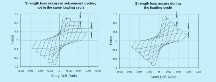
Cyclic Versus In-cycle Degradation
Hysteretic models used for nonlinear dynamic analysis should distinguish and account for “cyclic” versus “in-cycle” degradation of strength and stiffness. Cyclic degradation is an apparent loss in strength at a given deformation level under reverse cyclic loading that occurs due to concrete cracking, bond slip, the Bauschinger effect (in metals), etc. Under continued loading in one direction, the observed strength loss under cyclic loading is recovered at larger deformations. On the other hand, in-cycle degradation is the loss in strength that occurs under increasing deformations within one loading excursion of a cycle or under monotonic loading. In-cycle degradation displays a negative post-yield stiffness. In-cycle degradation in reinforced concrete and masonry components is generally due to concrete crushing, shear failure, buckling or fracture of reinforcement, and splice failures. In steel components, in-cycle degradation occurs due to local and/or lateral torsional buckling and rupture or fracture of steel. In practice, most components experience both types of degradation. Studies have shown that in-cycle degradation is more damaging and contributes to so-called ratcheting behavior under dynamic loading, which can ultimately lead to collapse. See FEMA 440.
to model shear effects is by adding a nonlinear shear spring in series with the axial-flexural model.
2.3 Model Parameters for Cyclic Loading
In modeling the hysteretic properties of actual elements for analysis, the initial stiffness, strength, and post-yield force-displacement response of cross sections should be determined based on principles of mechanics and/or experimental data, considering influences of cyclic loading and interaction of axial, shear, and flexural effects. Under large inelastic cyclic deformations, component strengths often deteriorate (Figure 2-3) due to fracture, crushing, local buckling, bond slip, orother phenomena. If such degradations are included through appropriate modifiers to the stiffness and internal forces, the model can simulate most regular materials and devices experiencing hysteretic behavior (Ibarra et al. 2005; FEMA 2009a). ASCE 41 provides guidelines for estimation of
stiffness, strength, and deformation limits in steel, reinforced concrete, masonry and wood members; base isolators; and energy dissipation components of moment frames, braced frames, shear walls, diaphragms, infills, and foundations. Shown in Figure 2-7 is an idealized force versus deformation relationship as defined in ASCE 41 for specifying the force and deformation parameters of nonlinear component models. In ASCE 41, the force-deformation relationship is intended to represent the cyclic envelope that reflects strength degradation due to cyclic loading (Sidebar 4). This is in contrast to the
monotonic curve that represents the response under monotonic loading. The cyclic envelope and monotonic backbone curves are similar in that each includes four important points of strength and associated deformation. Referring to Figure 2-7,
these points include: effective yield (point B), peak strength (point C), residual strength (point D), and ultimate deformation (point E). While ASCE 41 typically provides specific values to
Figure 2-6 – Cyclic versus in-cycle degradation (FEMA 2005).
Cyclic strength degradation In-cycle strength degradation Strength loss occurs in subsequent cycles;
define points B, C, and E, the descending slope between point C and D is less well defined. Since in most cases the descending slope is more gradual than implied in Figure 2-7, it may be more reasonable to define the descending branch between point C and E (or to a point between D and E), as illustrated by the dashed line in the figure.
Since models that capture cyclic degradation of the backbone curve are not yet common in commercial analysis software, in most cases it is appropriate to define modeling parameters to reproduce component cyclic envelope curves for tests or published criteria in ASCE 41, PEER/ATC 72-1 or other sources. Otherwise, the analyst should check that the software being used can represent the cyclic degradation of the backbone curve with appropriate hysteresis rules. In addition to distinctions between monotonic and cyclic response, another important attribute of hysteretic models is whether they capture so-called “cyclic” versus “in-cycle” deterioration (Sidebar 5). For materials and
members not documented in available literature, degradation of stiffness, strength and bond characteristics should be evaluated using principles of mechanics that are supported by test data; FEMA 440A provides additional recommendations on this topic.
2.4 Geometric Nonlinear Effects
Geometric nonlinear effects are caused by gravity loads acting on the deformed configuration of the structure, leading to an increase of internal forces in members and connections. These geometric nonlinear effects are typically distinguished between
P-d effects, associated with deformations along the members, measured relative to the member chord, and P-D effects, measured between member ends and commonly associated with story drifts in buildings. In buildings subjected to earthquakes,
P-D effects are much more of a concern than P-d effects, and provided that members conform to the slenderness limits for special systems in high seismic regions (e.g., special concrete or steel moment frames as defined in ASCE 7), P-d effects do not generally need to be modeled in nonlinear seismic analysis. On the other hand, P-D effects must be modeled as they can ultimately lead to loss of lateral resistance, ratcheting (a gradual build up of residual deformations under cyclic loading), and
Figure 2-7 – Generalized force-deformation curve (PEER/ATC 2010).
dynamic instability. Large lateral deflections (D) magnify the internal force and moment demands, causing a decrease in the effective lateral stiffness. With the increase of internal forces, a smaller proportion of the structure’s capacity remains available to sustain lateral loads, leading to a reduction in the effective lateral strength.
Shown in Figure 2-8 is an idealized base shear versus drift
curve of a cantilever structure with and without P-D effects. If the gravity load is large the stiffness reduction (shown by the negative slope KN) is significant and contributes to loss of
lateral resistance and instability. Therefore the gravity load-deformation (P-D) effect must be considered directly in the analysis, whether static or dynamic. This means that the gravity loads of the entire building must be present in the analysis, and appropriate P-D analysis techniques should be introduced in the structural model (Wilson 2002; Powell 2010). For nonlinear seismic analyses, ASCE 7 specifies a gravity load combination of 1.0D + 0.5L, where D is the building dead load and L is the specified live load, including allowance for live load reduction.
Figure 2-8 – Force-deformation curve with and without the P-D effect (PEER/ATC 2010).
2.5 Characterization of Model Parameters
and Uncertainties
Variability in calculated demand parameters arises due to uncertainties in the input ground motions and the nonlinear structural response to these motions (Sidebar 6). As the usual
approach in analysis is to obtain the most likely (expected) structural response, the structural properties used in the analysis model should be median values. The statistical variability in material parameters and model components generally follow a lognormal distribution, which implies that the median and mean (expected) values are not the same. However, as this difference is small for most material and other model parameters, combined with the fact that in practice there is rarely enough data to accurately characterize the difference, then it is reasonable to use either median or mean values to establish the parameters of the analysis model. This would include using median values of material properties and
component test data (such as the nonlinear hysteretic response data of a flexural hinge) to calibrate the analysis models. ASCE 41 and other standards provide guidance to relate minimum specified material properties to expected values, e.g., AISC 341 (AISC 2010) specifies Ry values to relate expected to minimum specified material strengths. By using median or mean values for a given earthquake intensity, the calculated values of demand parameters are median (50th percentile) estimates.
2.6 Quality Assurance
Nonlinear analysis software is highly sophisticated, requiring training and experience to obtain reliable results. While the analysis program’s technical users manual is usually the best resource on the features and use of any software, it may not provide a complete description of the outcome of various combinations of choices of input parameters, or the theoretical and practical limitations of different features. Therefore, analysts should build up experience of the software capabilities by performing analysis studies on problems of increasing scope and complexity, beginning with element tests of simple cantilever models and building up to models that encompass features relevant to the types of structures being analyzed. Basic checks should be made to confirm that the strength and stiffness of the model is correct under lateral load. Next, quasi-static cyclic tests should be run to confirm the nature of the hysteretic behavior, sensitivity tests with alternative input parameters, and evaluation of cyclic versus in-cycle degradation (Sidebar 5).
Further validations using published experimental tests can help build understanding and confidence in the nonlinear analysis software and alternative modeling decisions (e.g., effects of element mesh refinement and section discretization).
Beyond having confidence in the software capabilities and the appropriate modeling techniques, it is essential to check the accuracy of models developed for a specific project. Checks begin with basic items necessary for any analysis. However, for nonlinear analyses additional checks are necessary to help ensure that the calculated responses are realistic. Sidebar 7
gives some suggestions in this regard. Sidebar 6
Uncertainties in Seismic Assessment
The total variability in earthquake-induced demands
is large and difficult to quantify. Considering all major sources of uncertainties, the coefficients of variation in
demand parameters are on the order of 0.5 to 0.8 and generally increase with ground motion intensity. The variability is usually largest for structural deformations and accelerations and lower in force-controlled components of capacity-designed structures where the forces are limited by the strengths of yielding members. The variability is generally attributed to three main sources: (1) hazard uncertainty in the ground motion intensity, such as the spectral acceleration intensity
calculated for a specified earthquake scenario or return
period, (2) ground motion uncertainty arising from frequency content and duration of a ground motions
with a given intensity, and (3) structural behavior and
modeling uncertainties arising from the variability in (i) physical attributes of the structure such as material properties, geometry, structural details, etc., (ii) nonlinear behavior of the structural components and system, and (iii) mathematical model representation of the actual behavior. Through realistic modeling of the underlying mechanics, nonlinear dynamic analyses reduce uncertainty in demand predictions, as compared to nonlinear or linear static analyses where
the underlying uncertainties are masked by simplified
analysis assumptions. However, even with nonlinear dynamic analyses it is practically impossible to calculate accurately the variability in demand parameters. In concept it is possible to quantify the corresponding variability in the calculated demands using techniques such as Monte Carlo simulation. However, complete characterization of modeling uncertainty is a formidable problem for real building structures. Apart from the lack of necessary data to characterize fully the variability of the model parameters (standard deviations and correlations between multiple parameters), the number of analyses required to determine the resulting variability is prohibitive for practical assessment of real structures. Therefore, nonlinear analysis procedures are generally aimed at calculating the median (or mean) demands. Uncertainties in the evaluation are then accounted for
(1) through the choice of the specified hazard level
(return period) at which the analysis is run, and/or (2)
the specified acceptance criteria to which the demands
are compared. Separate factors or procedures are sometimes applied to check acceptance criteria for force-controlled or other capacity designed components.
Sidebar 7
Quality Assurance of Building Analysis Models
Beyond familiarizing oneself with the capabilities of a specific software package, the following are suggested checks
to help ensure the accuracy of nonlinear analysis models for calculating earthquake demand parameters:
Check the elastic modes of model. Ensure that the first mode periods for the translational axes and for
rotation are consistent with expectation (e.g., hand calculation, preliminary structural models) and that the sequence of modes is logical. Check for spurious local modes that may be due to incorrect element
properties, inadequate restraints, or incorrect mass definitions.
Check the total mass of the model and that the effective masses of the first few modes in each direction are
realistic and account for most of the total mass.
Generate the elastic (displacement) response spectra of the input ground motion records. Check that they are consistent and note the variability between records. Determine the median spectrum of the records and the variability about the median.
Perform elastic response spectrum (using the median spectrum of the record set) and dynamic response history analyses of the model, and calculate the displacements at key positions and the elastic base shear and overturning moment. Compare the response spectrum results to the median of the dynamic analysis results.
Perform nonlinear static analyses to the target displacements for the median spectrum of the ground motion record set. Calculate the displacements at key positions and the base shear and overturning moment and compare to the elastic analysis results. Vary selected input or control parameters (e.g., with and without P-D,
different loading patterns, variations in component strengths or deformation capacities) and confirm observed
trends in the response.
Perform nonlinear dynamic analyses and calculate the median values of displacements, base shear, and overturning moment and compare to the results of elastic and nonlinear static analyses. Vary selected input or control parameters (similar to the variations applied in the static nonlinear analyses) and compare to each other and to the static pushover and elastic analyses. Plot hysteresis responses of selected components to
confirm that they look realistic, and look for patterns in the demand parameters, including the distribution of
deformations and spot checks of equilibrium.
• • • • • •
3. Modeling of Structural Components
3.1 Moment Frames
(Flexural Beam-Columns)
Inelastic modeling of moment frame systems primarily involves component models for flexural members (beams and columns) and their connections. For systems that employ “special” moment frame capacity design principles, as defined in ASCE 7, the inelastic deformations should primarily occur in flexural hinges in the beams and the column bases. The NEHRP Seismic Design Technical Briefs by Moehle et al. (2008) and Hamburger et al. (2009) provide a summary of design concepts, criteria, and expected behavior for special concrete and steel moment frames. It is important to recognize, however, that the minimum design provisions of ASCE 7 and the underlying AISC 341 (2010) and ACI 318 (2008) standards for special moment frames do not always prevent hinging in the columns or inelastic panel zone deformations in beam-to-column joints. Therefore, the nonlinear model should include these effects, unless the actual demand-capacity ratios are small enough to prevent them. In frames that do not meet special moment frame requirements of ASCE 7, inelastic effects may occur in other locations, including member shear yielding, connection failure, and member instabilities due to local or lateral-torsional buckling.
Beam-columns are commonly modeled using either concentrated hinges or fiber-type elements. While the fiber elements generally enable more accurate modeling of the initiation of inelastic effects (steel yielding and concrete cracking) and spread of yielding, their ability may be limited to capture degradation associated with bond slip in concrete joints and local buckling and fracture of steel reinforcing bars and steel members. Concentrated hinge models, which can be calibrated to capture the overall force-deformation (or moment-rotation) response, including post-peak degradation, are often more
practical. Whatever the model type, the analysis should be capable of reproducing (under cyclic loading) the component cyclic envelope curves that are similar to those from tests or other published criteria, such as in ASCE 41 and PEER/ATC 72-1.
The inelastic response of flexural beams and columns is often linked to the response of the connections and joint panels between them. The inelastic behavior in the beams, columns, connections, and panel zone (Figure 3-1a) can each be modeled through the idealized springs, shown in Figure 3-1b (or equivalent fiber models), along with appropriate consideration of finite panel size and how its deformations affect the connected members. In steel structures, these yielding regions (beam, column, connections, and panel zone) tend to deform independently, except insofar as the strength of one component may limit the maximum forces in an adjacent component. On the other hand, in concrete frames, the inelastic deformations in the beams and columns are coupled with the panel zone behavior, due to the bond slip of longitudinal beam and column bars in the joint region. Thus, for concrete frames, the flexural hinge parameters should consider how the deformations due to bond slip are accounted for – either in the beam and column hinges or the joint panel spring. Depending on the specific software implementation, the finite-size joint panel may be modeled using kinematic constraint equations, equivalent bar-spring assemblies, or approximate rigid end offsets (Charney and Marshall 2006; ASCE 2007).
3.1.1. Steel Moment Frames
For steel frames that employ special seismic design and detailing, where the hinging locations are known and behavior is ductile, it is relatively straightforward to capture the response by nonlinear analysis, including hinging with P-M interaction and joint panel zone yielding. This would generally encompass
(b) Idealized analysis model (a) Hinging region of beams and columns
frames that conform to the special moment frame requirements of ASCE 7 and AISC 341 (Hamburger et al. 2009). Existing “pre-Northridge” moment frames, designed in high seismic regions of the Western U.S. according to older building code provisions, can be analyzed with similar models, provided that the beam/connection hinge ductility is reduced to account for potential fractures at the beam-to-column connection. Similarly, with appropriate adjustments to simulate the nonlinear moment-rotation behavior of connections, frames with partially restrained connections can be modeled. For steel frames composed of members with slender section properties and/or long unbraced lengths, nonlinear modeling is significantly more challenging due to the likelihood of local flange or web buckling and lateral-torsional buckling. This, combined with the fact that the inelastic rotation capacity of slender members is small, generally makes it less advantageous to use inelastic analysis for the design of steel frames with slender members. ASCE 41 provides some criteria for seismically non-conforming steel members, but as the cases covered are limited, one would need to look to other sources for data to establish models and criteria for frames with slender and otherwise non-conforming members.
3.1.2 Concrete Moment Frames
Concrete frames that meet seismic design and detailing requirements and qualify as special moment frames are somewhat more difficult to model than steel frames. Stiffness of members is sensitive to concrete cracking, the joints are affected by concrete cracking and bond slip, and the post-yield response of columns and joint panels is sensitive to axial load. ASCE 41 (including supplement 1) and PEER/ATC 72-1 provide models and guidance for characterizing member stiffness, inelastic member hinge properties, and strategies for joint modeling. Lowes and Altoontash (2003) and Ghobarah and Biddah (1999) provide further details on modeling concrete beam-column joints. Frames that do not conform to the special seismic detailing but have behavior that is dominated by flexural
hinging can also be modeled, provided that the hinge properties and acceptance criteria are adjusted to account for their limited ductility. Frames with members that are susceptible to sudden shear failures or splice failures are more challenging to model. In such cases, nonlinear flexural models can be used to track response only up to the point where imposed shear force and/ or splice force equals their respective strengths. Otherwise, to simulate further response, the analysis would need to capture the sudden degradation due to shear and splice failures.
3.2 Braced Frames
Modeling of inelastic brace behavior is complicated by the interactive effects of yielding, overall member buckling, local buckling, and fracture. For example, shown in Figure 3-2 is the
hysteretic plot and photo of a steel brace, tested under a cyclic loading protocol. As indicated, the compression behavior is dominated by global buckling with rapid drop off in strength and recovery of the tensile yield strength upon reloading. Compression buckling typically leads to a concentration of flexural hinging at the mid-point of the brace, where under increased deformations local buckles form, which then trigger fracture during subsequent tension cycles.
There are several alternatives for modeling the nonlinear buckling response of braces. A commonly employed approach is to model the brace with fiber beam-column elements, which capture yielding, overall buckling, and concentration of plastic rotations in the buckled hinge, provided the number of elements along the length of the brace is adequate. Local buckling and fracture can be inferred from the plastic rotation and strains in the hinges (Uriz and Mahin 2008). In an alternative model, the brace is represented by a uniaxial phenomenological spring to capture brace yielding and overall buckling (e.g., Tang and Goel 1989; Uriz and Mahin 2008). This type of element is simple to use, though its reliability is more limited by the range of tests to which it is calibrated. In the most fundamental
Figure 3-2 – Nonlinear response of axial brace (Fell et al. 2010).
(b) Experimental set-up (a) Measured axial force-deformation
analysis approach, the brace is modeled with continuum finite elements which can directly simulate yielding, overall buckling, and local buckling (Schachter and Reinhorn 2007). With appropriate material formulation, the finite element models can also simulate fracture initiation (Fell et al. 2010).
The axial-flexural fiber model, which provides a good compromise between modeling rigor and computational demands, requires calibration with test data to determine the appropriate number of elements, amplitude of initial out-of-straightness imperfections, and material hardening parameters. Uriz and Mahin (2008) found that the fiber approach gave reasonable results for the following model parameters: (1) brace subdivided into two or four elements, (2) initial geometric imperfection amplitude of 0.05 % to 0.1 % of the member length, and (3) ten to fifteen layers (fibers) through the cross section depth. For braces with compact sections as specified by AISC 341, local buckling is usually delayed enough to be insignificant until large deformations (story drifts on the order of 2 % to 4 %, depending on the brace compactness and slenderness). ASCE 41 provides acceptance criteria, described as a function of axial brace displacements, which can be obtained from the fiber-type beam-column models, phenomenological axial spring models, or finite element models.
3.2.1 Buckling-Restrained Braces
In contrast to conventional braces, buckling-restrained braces are straightforward to model with uniaxial nonlinear springs. Yield strength, cyclic strain hardening, and low-cycle fatigue endurance data are generally available from the brace manufacturers. Bi-linear force-deformation models are sufficiently accurate to capture the behavior. Acceptance criteria for the brace elements, based on peak deformations and cumulative deformations, can be inferred from the AISC 341 qualification testing requirements for buckling restrained braces.
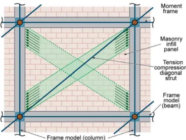
3.3 Infill Walls and Panels
Although not widely employed for new construction in high seismic regions of the U.S., frames with infill walls are commonly encountered in existing buildings around the world and in regions of low to moderate seismicity of the U.S. The infill wall system is conventionally modeled as a frame structure with beams and columns braced with one or two diagonal struts representing the masonry infill (Figure 3-3). In most cases, the infill panel failure will initiate in sliding along the horizontal joints, where the capacity is limited by the shear strength of the mortar. Alternatively, if the panel is strong in shear, the diagonal strut will crush near the frame joint and lose strength. This mode of failure has limited deformation capacity because the crushing will be abrupt. The large panel forces generated in this mode will be distributed along the beam and column
members, and they may result in either column or beam shear failures. Depending on their height-to-thickness slenderness, unreinforced infill walls can also fail out-of-plane, sometimes in combination with one of the other modes.
For either the shear sliding or compression crushing mode, it is reasonable to analyze frames with infills using a single equivalent strut or two diagonal compression struts for reversed cyclic loading analysis. Such an approach is adopted by FEMA 306 (FEMA 2009b) and ASCE 41. Detailed finite element analysis can also be used if such a refinement is required, but it presents challenges both in terms of computational demands and constitutive modeling of the infill and boundary interface. For software that supports use of a single axial spring, the spring strength should be based on the governing failure mode (sliding or compression failure). Madan et al. (1997) provides an example of a more advanced series spring strut model, which captures the combined behavior of diagonal sliding shear and compression failure, including cyclic deterioration. Kadysiewski and Mosalam (2009) provides a modeling approach that considers both in-plane and out-of-plane failure.
Modeling of the equivalent diagonal strut requires knowledge of the stiffness and cyclic strength behavior. The equivalent strut is represented by the actual infill thickness that is in contact with the frame, the diagonal length, and an equivalent width which may be calculated using the recommendations given in the concrete and masonry chapters of ASCE 41. Only the masonry wythes in full contact with the frame elements should be considered when computing in-plane stiffness, unless positive anchorage capable of transmitting in-plane forces from frame members to all masonry wythes is provided on all sides of the walls.
3.4 Shear Walls
Reinforced concrete shear walls are commonly employed in seismic lateral-force-resisting systems for buildings. They may take the form of isolated planar walls, flanged walls (often C-, I- or T-shaped in plan) and larger three dimensional assemblies such as building cores. Nearby walls are often connected by coupling beams for greater structural efficiency where large openings for doorways are required. The seismic behavior of shear walls is often distinguished between slender (ductile flexure governed) or squat (shear governed) according to the governing mode of yielding and failure. In general, it is desirable to achieve ductile flexural behavior, but this is not possible in circumstances such as (1) short walls with high shear-to-flexure ratios that are susceptible to shear failures, (2) bearing walls with high axial stress and/or inadequate confinement that are susceptible to compression failures, and (3) in existing buildings without seismic design and detailing qualifying the wall system as special as defined in ASCE 7. Cyclic and shake table tests on reinforced concrete shear walls reveal a number of potential failure modes that simple models cannot represent explicitly, however these failure modes are generally reflected in the backbone curves, hysteresis rules, and performance criteria adopted in lumped plasticity models. These failure modes include (1) rebar bond failure and lap splice slip, (2) concrete spalling, rebar buckling, and loss of confinement, (3) rebar fracture on straightening of buckle, and (4) combined shear and compression failure at wall toe. Some of these failure modes can be captured, either explicitly or implicitly, in fiber and finite element type modeling approaches.
3.4.1 Modeling of Slender Walls
Slender concrete shear walls detailed to current seismic design requirements, having low axial stress, and designed with sufficient shear strength to avoid shear failures, perform in a similar manner to reinforced concrete beam-columns. Ductile flexural behavior with stable hysteresis can develop up to hinge rotation limits that are a function of axial load and shear in the hinge region.
Subject to the cautions noted below, simple slender walls (including coupled walls) can be modeled as vertical beam-column elements with lumped flexural plastic hinges at the ends with reasonable accuracy and computational efficiency. The modeling parameters and plastic rotation limits of ASCE 41 may be used for guidance. The following points should be noted:
The lumped hinge models are only suitable for assessing performance within such allowable plastic hinge rotation limits as stable hysteresis occurs, considering axial and shear forces in the hinge.
Nonlinearity only arises at the designated hinge(s), and equivalent flexural and shear stiffness must be specified for elastic elements outside of the hinge. ASCE 41 and PEER/ATC 72-1 provide guidance on effective stiffness parameters that account for flexural and shear cracking to handle typical cases (i.e., planar walls with typical reinforcement, wall proportions, and gravity stresses). The flexural strength may be estimated by the nominal strength provisions of ACI 318 using expected material properties and taking account of the axial load. Where the axial load varies significantly during loading (e.g., coupled shear walls) a P-M interaction surface (Figure 2-2) should be used rather than a constant flexural strength.
Shear failure should be prevented in slender shear walls, and studies have shown (PEER/ATC 72-1) that standard seismic design criteria may underestimate the actual shear force demands. Therefore, it is best to perform the analysis to determine the shear force demands and then to design the wall to resist these demands, considering variability in the shear demands and capacities. Since shear strength varies with applied axial stress (which varies during an earthquake in coupled shear walls) it may be necessary to check the design at multiple time steps during nonlinear dynamic analyses.
Beam-column elements are more problematic to use in three-dimensional wall configurations with significant bi-directional interaction, particularly if the wall system is subjected to torsion.
Fiber-type models are commonly employed to model slender walls, where the wall cross section is discretized into a number of concrete and steel fibers. With appropriate material nonlinear axial stress-strain characteristics, the fiber wall models can capture with reasonable accuracy the variation of axial and flexural stiffness due to concrete cracking and steel yielding under varying axial and bending loads. A principal limitation of conventional beam-column element fiber formulations is the assumption that plane sections remain plane, such that shear lag effects associated with flexure and warping torsion are not captured. These effects may be significant in non-planar core wall configurations. This limitation may be alleviated through formulations that model the wall with two-dimensional shell-type finite elements. The fiber idealization can be implemented in the shell elements to integrate through the cross section for axial/flexural effects, but in-plane shear is uncoupled and remains elastic. The number of elements required across a wall segment width and over the wall height depends on the available element types, the wall proportions, and the bending moment gradient. In particular, the number of elements over the hinge length will impact the effective gage length of the calculated strains. • • • • •