Using Python for Signal Processing and Visualization

Using Python for Signal Processing and Visualization

Abstract

We describe our efforts on using Python, a powerful intepreted language for the signal processing and visualization needs of a neuroscience project. We use a Python-based approach to put together complex data processing and advanced visualization techniques into a coherent framework.

1

Introduction

An ever-increasing number of scientific studies are generating larger, more complex, and multi-modal datasets. This results in data analysis tasks becoming more demanding. To help tackle these new chal-lenges, more disciplines now need to incorporate advanced visualization techniques into their standard data processing and analysis methods. While many systems have been developed to allow scientists to explore, analyze, and visualize their data, many of these solutions are domain specific, limiting their scope as general processing tools. One way to enhance their flexibility is to built on top of an interpreted language.

The Python programming language [9] provides a development environment suitable to both compu-tational and visualization tasks. One of the key advantages of Python is that packages can be used to extend the language to provide advanced capabilities such as array and matrix manipulation [5], image processing [12], digital signal processing [5], and visualization [7]. Several popular data exploration and visualization tools have been built in Python, including VisIt (www.llnl.gov/visit), Paraview (www.paraview.org), CDAT (esg.llnl.gov/cdat) and VisTrails (www.vistrails.org). In our work, we use VisTrails; however, nearly any Python-enabled application would be capable of producing similar results.

A Neuroscience Example

The field of Neuroscience often uses both multi-modal data as well as computationally complex algorithms to analyze data collected from participants in a study. Here we investigate a study in which Magnetic Resonance Imaging (MRI) is combined with Electroencephalography (EEG) to examine working memory. The MRI provides a three-dimensional depiction of the structure of the brain and presents a natural spatial organization for the EEG sensors. EEG data is collected from 64 sensors placed on the scalp. These sensors measure the voltages at the scalp generated by brain activity.

Working memory is generally thought of as the neural assemblies governing short-term retention of in-formation and the integration of this data into the executive decision making process. It has been shown that brain activity regarding working memory is spectrally and spatially organized [10]. Specifically, working memory performance can be assessed by measuring changes to the energy densities, phase relationships, and frequency shifts in the alpha band of frequencies (7–13 Hz), located in the dorsal-lateral pre-frontal

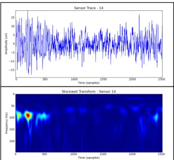
Figure 1: (Top) A plot of a single sensor’s raw data trace. (Bottom) The S-Transformed representation of the sensor’s raw data. Since this visualization shows all representable frequencies at each timestep, this view allows the time series’ frequency evolution to be analyzed.

cortex. To analyze the temporal and spectral organization of working memory, advanced signal process-ing techniques are employed to transform the time series gathered from EEG sensors in specific locations into Fourier-based representations. As the sensor locations are known, spatial representations of various EEG-based quantities are implied, but difficult to see.

The use of MRI data with the known EEG sensor locations highlights spatial relationships between the sensors and the brain activity they measure. During more complex analysis, MRI data is often used to de-termine participant-specific finite element meshes for use in solving the inverse problem, assigning scalar values to the cortical surface based on data collected at sensor locations more robustly than interpolation schemes. Solving the inverse problem in this way is useful for tasks such as source localization for epilep-togenic regions of the brain. Fortunately, for determining spatial relationships between active brain regions and EEG sensors, radial basis function interpolation has proven to be a good approximation [4]. Regardless of the method by which scalars are mapped from discrete point locations to a surface representation, data collected from different acquisition methods must be fused into a coherent representation. However, for this type of data fusion to be performed, the MRI data must first be registered with the EEG sensor locations. Furthermore, segmentation of the MRI to extract the brain surface onto which scalar values derived from the EEG will be mapped must be performed.

The study discussed here culminates in a visualization depicting the spectral power at the alpha band of frequencies (7–13Hz) across the entire cortical surface. Additionally, the time-frequency representation for each sensor’s data must be selectable to provide details when queried. This task requires the use of signal processing techniques to decompose the EEG data, image processing techniques to segment the brain surface from the MRI, interpolation techniques to approximate the brain surface activity responsible for the EEG data, as well as 1-, 2-, and 3-D rendering techniques for the presentation of the data.

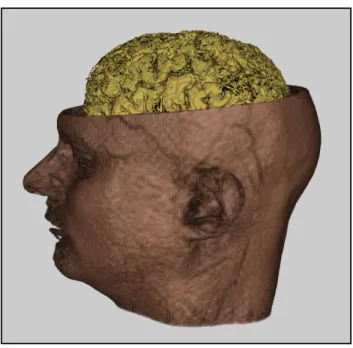
Figure 2: Registering sensor locations with MRI-based data reveals the spatial relationships between the EEG sensors and the structures evident in the MRI volume.

2

EEG Signal Processing

In order to process EEG data for interpretation and further analysis, Fourier-based transforms can be used to determine spectral properties of brain activity. Determining how spectral properties change over time is important to the study of working memory. The need for these techniques stems from the assessment of working memory performance through the change in specific spectral properties of the EEG signals mea-sured at the scalp. When working memory is tasked, alpha-band power increases while simultaneously shifting to slightly higher frequencies. Fast Fourier Transforms (FFTs), various filters, and some wavelet implementations are distributed with the Scipy Python package to help accomplish this goal. FFT computa-tion is fast within Scipy as it makes use of the FFTW libraries [2]. However, standard FFTs are not adequate when analyzing the evolution of spectral content over time.

When examining the temporal aspects of a time series’ frequency-based representations, several dif-ferent transformations are applicable. One time frequency decomposition, Short-Time Fourier Transforms (STFTs) use time windows to examine spectral evolution. STFTs suffer from a uniform packing of the time-frequency space. Alternatively, wavelet-based approaches use an adaptive resolution scheme to pack the time-frequency space, but lack a direct mapping from scale to frequency. On the other hand, the Stockwell Transform [8] uses an adaptive resolution scheme similar to Wavelet Transforms, but still maintains a direct mapping to the frequency domain. Figure 1 shows the results of a Stockwell transform representing the energy density between 1 and 250 Hz during the course of an experiment.

We have chosen to use Stockwell Transforms throughout our analysis. Since other time-frequency representations can be used to analyze this dataset, the processing pipeline must be easily changeable to accomodate different Fourier-based decompositions. This type of flexibility is important when exploring not just time series data, but the different data products resulting from processing and analysis. Using

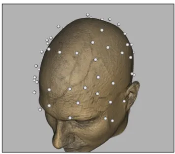
Figure 3: Registering sensor locations with MRI-based data reveals the spatial relationships between the EEG sensors and the structures present in the MRI volume.

Python as the underlying framework for data analysis provides an easy way of changing analyses on-the-fly using a range of implementations from user-created specifications to robust, compiled libraries.

Unfortunately, Stockwell Transforms are computationally intensive and compiled languages generally perform better than interpreted languages in this situation. To accelerate the computation of the transform, it was implemented in optimized C (available athttp://kurage.nimh.nih.gov/meglab/Meg/Stockwell). This small C li-brary is made accessible to Python by the use of compiled bindings. Using compiled Python bindings allows methods written in C or C++ to be usable by Python. These bindings can also be generated in Python directly using thectypespackage (http://docs.python.org/library/ctypes.html). Wrapping methods with Python bindings al-lows code execution to be performed in faster compiled languages lending additional speed to Python-based applications. This execution method makes computationally intense algorithms tractible inside an inter-preted language environment.

3

Volume Segmentation and Registration

Once EEG data is processed and analyzed, structural information must be extracted from the MRI volume collected. Segmentation of such volumes is a difficult task, best suited for specialty libraries and algo-rithms [11]. We have employed the Insight Toolkit (ITK) [12] to extract the brain area from the MRI data. ITK is a collection of image processing algorithms implemented in C++ that provide volumetric opera-tions from smoothing to segmentation. As with many other libraries, ITK is distributed with a collection of Python bindings. In the case of ITK, this is done automatically by Kitware’s CableSwig, which provides a mechanism to wrap highly templated C++ libraries for use with Python. Without CableSwig, the templated nature of ITK would generate an unnecessarily large number of bindings, complicating its use in Python.

We are using ITK here because we need to segment the MRI volume. To simplify this procedure, we decided to use the automatic cortical extraction method of Prastawa et al. [6]. After segmentation,

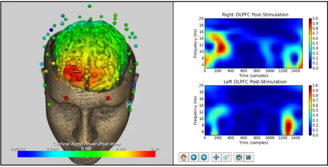
Figure 4: Data processing and visualization performed in Python results in interactive viusalizations of multi-modal data. Here we see alpha-band activity (7–13 Hz) in the frontal regions of the brain (left). Specific time-frequency representations are determined by the user-driven selection of EEG sensors (right). This is consistant with known patterns described in literature [3].

an iso-surface of the cortex was extracted to augment the MRI visualization by embedding the surface in a traditional volume rendering. Figure 2 shows the result of this automatic segmentation. Spatial relationships between different structures are revealed by combining the clipped MRI volume with the extracted cortical surface.

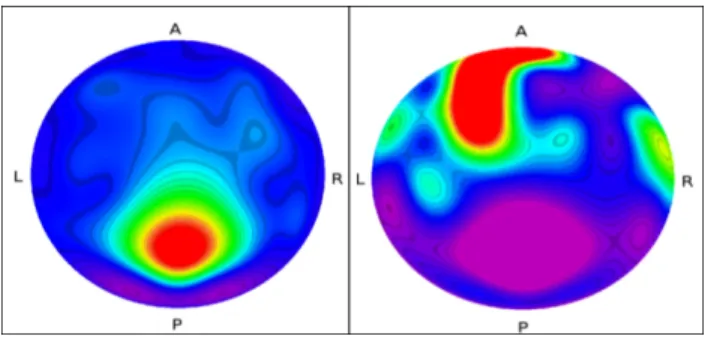
Visualizations of this nature make it easier to analyse the data. In particular, correlations between spatial relationships of brain structures and brain activity measured by EEG are highlighted by this type of multi-modal visualization. One way spatial relationships are visualized is through the use of topographic maps (topomaps). This method uses a surrogate representation of the scalp and places values on it based on the EEG data collected. Figure 5 shows two timesteps in the experiment, but does not take into account the three dimensional nature of the MRI data. By registering the MRI volume, cortical surface, and sensor locations provided by the EEG manufacturer, a cohesive representation of the entire dataset is formed respecting the individual structures measured by the MRI. Figure 3 shows the dataset after the 3D registration of the MRI volume and sensor locations is performed.

4

Visualization

We use the VTK library for our visualization tasks. This C++ library provides advanced visualization capabilities to Python programs. In this way, we are able to combine volume rendering, surface rendering, and point rendering for the MRI volume, cortical surface, and registered sensor locations, respectively. However, additional processing must be performed to properly map scalar values onto the cortex.

Figure 5: Topographic maps generated from EEG data projected onto a surrogate head provide some spa-tial indications of brain activity. Here, the topomaps are colored based on average alpha power when a participant is in a resting state (left) and during a working memory task (right). The surrogate head model represents only data collected and interpolated onto the scalp making no attempt at mapping values to the cortical surface.

In this way, we are able to approximate scalar values on the cortical surface given values at each sensor location. While this method is not equivalent to a solution of the inverse problem, it provides a good estimate of the spatial organization of brain activity. Figure 4 shows the results of applying RBF interpolation for the average power in the alpha band of frequencies (7–13 Hz) measured at each sensor location.

VTK also provides functionality for selection and on-the-fly updates to enhance interaction. It is through this mechanism that we are able to select individual sensors and display their unique time-frequency rep-resentations. Instead of displaying the 2D time-frequency planes using VTK, use the Pylab plotting func-tionality distributed with SciPy. Pylab specializes in 1- and 2-dimensional plotting techniques, and proves to be an ideal rendering library for time-frequency data. While the left portion of Figure 4 shows 3D data rendered using VTK, the right side uses Pylab to visualize the time-frequency planes of the selected sensors.

5

Discussion

Tools allowing rapid exploration of large and multi-modal datasets are more important than ever in scientific research. Interpreted languages, like Python, provide a solid foundation for the development of powerful, yet flexible data analysis and visualization tools. However, flexibility of analysis and visualization must be combined to enhance the exploration process. Our Python system was implemented as a series of VisTrails Python Modules [1]. The VisTrails system is a visual programming paradigm in which computational elements are represented by drag-and-drop modules that are connected together to form programs. The drag-and-drop system makes replacing functionally equivalent computations, such as replacing an STFT with a Stockwell Transform, easy to do.

Providing a tool that supports flexible visualization and analysis allows scientists to draw more insightful conclusions. Additionally, the ability to change analysis techniques enables important insights to be gained more quickly. Using visual programming paradigms, like VisTrails, makes changing analysis techniques easier for non-programmers, facilitating the use of the tool for insight generation.

In addition to making changes to analysis techniques easier, Python has also proven to be excellent at combining related, yet disparate data into a single, useful representation. This data fusion is exemplified in Figure 4 which has successfully combined structural volumetric data with processed time series data. When

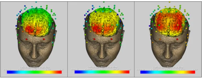
Figure 6: Rendering multiple time-steps of this data depicts the underlying neural circuit associated with working memory. In this case, activity spreads throughout the cortex moving between the dorso-lateral pre-frontal cortex (left), the temporal region (middle), and the parietal areas (right). This series of images taken from an animation highlights not just the spectral and temporal organization of working memory, but also it’s spatial coherence. Without adequate visualization techniques, the link between memory and specific regions of the brain would be more difficult to determine.

animated, visualziations (Figure 6) show not just the activity of the brain, but how it evolves spectrally and spatially throughout the cortex. Analysis taking spatial data into account is common in neuroscience; however, most of these techniques respect spatial relationships by scientists selecting groups of sensors located at specific places to focus their analysis efforts. Providing methods to neuroscientists the ability to examine their dataset as a whole allows insightful analysis to be performed more quickly. The efficiency gained by better utilizing visualization as a tool stems from new and unexpected behavior being identified more easily.

6

Conclusions

We have presented a small case-study of the use of Python as a foundation for the exploration and analysis of multi-modal data. Python’s large user community and array of libraries enhance the language by providing new functionality useful in every aspect of data processing and management. The availablity, flexibility, and ease of use of this language facilitates scientific endeavors from computationally intense applications to colalborative analysis.

The Python programming language provides a strong foundation on which flexible applications are built. Leveraging optimized C, C++, and even FORTRAN libraries through wrapping them for use in Python allows applications to be both flexible and powerful. Additional open-source libraries supported by Python, such at Qt (http://qt.nokia.com), provide powerful user interface capabilities for any application to use.

Python is not alone in its use of compiled libraries. Other interpreted languages also take advantage of external libraries to overcome execution speed barriers. Probably the most notable of these languages is MATLAB. While MATLAB and Python are largely equivalent in terms of their capabilities, Python is open-source, making it quite an attractive solution to many applications. Applications developed in Python

can be widely distributable, making it easier to enable collaboration between scientists at various locations.

Acknowledgements

Working versions and source code for the material in this article can be obtained fromwww.vistrails.org. This work was supported in part by grants from the National Science Foundation, the National Institutes of Health, the Department of Energy, and IBM Faculty Awards.

References

[1] L. Bavoil, S. P. Callahan, P. J. Crossno, J. Freire, C. E. Scheidegger, C. T. Silva, and H. T. Vo. VisTrails: Enabling interactive multiple-view visualizations. Proceedings of IEEE Visualization, 2005.

[2] M. Frigo and S. G. Johnson. FFTW: An adaptive software architecture for the FFT. Proceedings of ICASSP, 3:1381–1384, 1998.

[3] W. Klimesch. EEG alpha and theta oscillations reflect cognitive and memory performance: a review and analysis. Brain Research Reviews, 29(2–3), 1999.

[4] M. R. Nuwer. Quantitative EEG: Techniques and problems of frequency analysis and topographic mapping. Journal of Clinical Neurophysiology, 5(1), 1988.

[5] T. E. Oliphant. Python for scientific computing. Computing in Science and Engineering, 9:10–20, 2007.

[6] M. Prastawa, J. H. Gilmore, W. Lin, and G. Gerig. Automatic segmentation of MR images of the developing newborn brain. Medical Image Analysis, 9, 2005.

[7] W. Schroeder, K. Martin, and B. Lorensen. The Visualization Toolkit, Third Edition. Kitware Inc., 2004.

[8] R. G. Stockwell. A basis for efficient representation of the S-transform. Digital Signal Processing, 2006.

[9] G. van Rossum. Python tutorial. Technical Report CS-R956, Centrum voor Wiskunde en Informatica (CWI), 1995.

[10] A. von Stein and J. Sarnthein. Different frequencies for different scalees of cortical integration: from local gamma to long range alpha/theta synchronization. International Journal of Psychophysiology, 38(3), 2000.

[11] H. Xue, L. Srinivasan, S. Jiang, M. Rutherford, A. D. Edwards, D. Rueckert, and J. V. Hajnal. Auto-matic segmentation and reconstruction of the cortex from neonatal MRI. NeuroImage, 38(3), 2007.

[12] T. S. Yoo, M. J. Ackerman, W. E. Lorensen, W. Schroeder, V. Chalana, S. Aylward, D. Metaxas, and R. Whitaker. Engineering and Algorithm Design for and Image Processing API: A technical report on ITK – The Insight Toolkit. Proceedings of Medicine Meets Virtual Reality, pages 586–592, 2002.